Essays on Alternative Perspectives on Cross Border B2B Trust and Commitment

Computer Science Dissertations Department of Computer Science

8-7-2018

Assembly, quantification, and downstream analysis

for high trhoughput sequencing data

Igor Mandric

Follow this and additional works at:https://scholarworks.gsu.edu/cs_diss

This Dissertation is brought to you for free and open access by the Department of Computer Science at ScholarWorks @ Georgia State University. It has been accepted for inclusion in Computer Science Dissertations by an authorized administrator of ScholarWorks @ Georgia State University. For more information, please [email protected].

Recommended Citation

Mandric, Igor, "Assembly, quantification, and downstream analysis for high trhoughput sequencing data." Dissertation, Georgia State University, 2018.

THROUGHPUT SEQUENCING DATA

by

IGOR MANDRIC

Under the Direction of Alexander Zelikovsky, PhD

ABSTRACT

Next Generation Sequencing is a set of relatively recent but already well-established

technologies with a wide range of applications in life sciences. Despite the fact that they

are constantly being improved, multiple challenging problems still exist in the analysis of

high throughput sequencing data. In particular, genome assembly still suffers from inability

of technologies to overcome issues related to such structural properties of genomes as single

genomes. Other types of issues arise in transcriptome quantification and differential gene

expression analysis. Processing millions of reads requires sophisticated algorithms which

are able to compute gene expression with high precision and in reasonable amount of time.

Following downstream analysis, the utmost computational task is to infer the activity of

biological pathways (e.g., metabolic). With many overlapping pathways challenge is to infer

the role of each gene in activity of a given pathway. Assignment products of a gene to

a wrong pathway may result in misleading differential activity analysis, and thus, wrong

scientific conclusions. In this dissertation I present several algorithmic solutions to some of

the enumerated problems above. In particular, I designed scaffolding algorithm for genome

assembly and created new tools for differential gene and biological pathways expression

analysis.

THROUGHPUT SEQUENCING DATA

by

IGOR MANDRIC

A Dissertation Submitted in Partial Fulfillment of the Requirements for the Degree of

Doctor of Philosophy

in the College of Arts and Sciences Georgia State University

THROUGHPUT SEQUENCING DATA

by

IGOR MANDRIC

Committee Chair: Alexander Zelikovsky

Committee: Robert Harrison

Pavel Skums Ion M˘andoiu Artem Rogovskyy

Electronic Version Approved:

DEDICATION

ACKNOWLEDGEMENTS

I would like to thank my scientific advisor Dr. Alex Zelikovsky for his wise guidance through my Ph.D. journey. His encouragement and support were very valuable during all these years. My passion and interest for bioinformatics are truly indebted to him.

I would also like to thank the Ph.D. committee members Dr. Pavel Skums, Dr. Ion Mandoiu, Dr. Artem Rogovskyy, and Dr. Robert Harrison.

I am very grateful to Dr. Rajsekhar Sunderraman, Dr. Xiaojun Cao, and Mrs. Tammie Dudley. They offered me invaluable help and support in many difficult situations.

Not of less importance for me was the collaboration with my colleagues. I would like to thank my older fellows Dumitru Brinza and Serghei Mangul. The latter was for me a tremendous example of energy and optimism. I am very happy I was a part of the same scientific group with my lab-mates Ekaterina Nenastyeva, Nick Mancuso, Olga Glebova, Pelin Icer, Sergey Knyazev, Andrew Melnyk, and others.

I would like to express my gratitude to the Faculty of Mathematics and Informatics of Moldova State University and especially to my Master advisor Dr. Dumitru Lozovanu. I can not help but mention my best friend Radu Buzatu who is also now a faculty member at the same university.

TABLE OF CONTENTS

ACKNOWLEDGEMENTS . . . v

LIST OF TABLES . . . ix

LIST OF FIGURES . . . xii

LIST OF ABBREVIATIONS . . . xix

PART 1 INTRODUCTION . . . 1

1.1 Background . . . 2

1.1.1 NGS technologies . . . 2

1.1.2 Bioinformatics Pipeline for NGS Data Analysis . . . 3

1.2 Problems . . . 4

1.3 Contributions . . . 7

1.4 Roadmap . . . 9

1.5 Scientific Products . . . 9

1.5.1 Publications . . . 9

1.5.2 Presentations . . . 11

1.5.3 Software Packages . . . 12

PART 2 ALGORITHMS FOR SCAFFOLDING AND SCAFFOLD-ING EVALUATION . . . 13

2.1 Introduction . . . 13

2.2 ScaffMatch: combinatorial optimization approach to genome scaf-folding . . . 18

2.2.1 Results . . . 25

2.3.1 Background . . . 32

2.3.2 Exact scaffolding evaluation . . . 35

2.3.3 Repeat-aware validation of scaffolders. . . 37

2.4 Repeat aware scaffolding . . . 47

2.4.1 Repeat and Short Contig Filtering Problem . . . 49

2.4.2 Results . . . 57

PART 3 ORF ASSEMBLY . . . 62

3.1 Introduction . . . 62

3.2 DORFA: Database-guided ORFeome Assembly method from RNA-Seq Data . . . 64

3.2.1 Methods . . . 64

3.2.2 Results . . . 68

PART 4 INFERENCE OF GENE EXPRESSION AND PATHWAY ACTIVITY LEVELS FROM RNA-SEQ DATA . . . . 70

4.1 Introduction . . . 70

4.2 IsoEM2: Quantification and Differential Expression Analysis of Gene and Isoform Expression from RNA-Seq data . . . 71

4.2.1 Software Features of IsoEM2 . . . 72

4.2.2 Experimental Results . . . 73

4.3 Metabolic Pathways Activity Levels: Inferring Relative Abundance and Differentially Expressed Pathways from RNA-Seq data . . . 75

4.3.1 Methods . . . 76

4.3.2 Results . . . 81

PART 5 IMMUNE REPERTOIRE PROFILING . . . 86

5.2 ImReP: CDR3 sequence assembly and profiling immune repertoires

from RNA-Seq data . . . 88

5.2.1 Methods . . . 88

5.2.2 Results . . . 91

LIST OF TABLES

Table 1.1 NGS technologies and their characteristics [13]. . . 3

Table 2.1 Scaffolding Datasets . . . 26

Table 2.2 Performance of different algorithms on the scaffolding datasets from

GAGE.. . . 27

Table 2.3 Performance of different algorithms on the scaffolding datasets for P.

falciparum. . . 28

Table 2.4 The wall clock runtime in seconds for the largest and the smallest

datasets. All scaffolders were run on 2.5GHz 16-core AMD Opteron

6380 processors with 256Gb RAM running under Ubuntu 12.04 LTS.

SM is ScaffMatch and SM G is ScaffMatch G. . . 29

Table 2.5 The number of unique contigs and the number of repeats in three

GAGE [76] datasets (S. aureus, R. sphaeroides, H. sapiens (chr 14))

and two fungi datasets (M. fijiensis, M. graminicola) obtained with

the aid of iWGS pipeline [102]. Each contig dataset is obtained with

the scripts from [40] from Velvet assembly contigs. . . 33

Table 2.6 The number of links classified as correct and incorrect by [40] when

applied to the perfect scaffoldings for three datasets S. aureus, R.

Table 2.7 Comparison between artificial contigs produced based on Velvet and

Allpaths-LG contigs. “# all contigs” – total number of contigs in the

dataset; “# common contigs” – in Velvet (Allpaths-LG) column,

num-ber of Velvet (Allpaths-LG) contigs which are either identical, or

con-tain one or more Allpaths-LG (Velvet) contigs, or are concon-tained in an

Allpaths-LG (Velvet) contig; “total contig length” – total length of all

contigs in the dataset; “common contig length” – in Velvet

(Allpaths-LG) column, total length of Velvet (Allpaths-(Allpaths-LG) contigs which are

either identical, or contain one or more Allpaths-LG (Velvet) contigs,

or are contained in an Allpaths-LG (Velvet) contig; “reference length”

– the length of the S. aureus genome; “JS divergence between copy

number profiles” – Jensen-Shannon divergence computed between the

distributions of copy numbers for the two datasets. . . 40

Table 2.8 The number of unique contigs and the number of repeats in three

GAGE [76] datasets (S. aureus, R. sphaeroides, H. sapiens (chr 14))

and two fungi datasets (M. fijiensis, M. graminicola) obtained with

the aid of iWGS pipeline [102]. Each contig dataset is obtained as

described in Section 2.3.3 (α = 0.97, λ= 200). . . 41

Table 2.9 The main parameters of the five datasets used in the experiments. 42

Table 2.10 The average wall clock runtime of the scaffolding validation and the

average wall clock time of the ILP (1) in seconds on the output

scaf-foldings obtained for the five datasets. As it can be clearly seen, most

of the validation time is spent on building the ILP itself and a

non-significant part is required for ILP to be solved. . . 45

Table 2.11 The evaluation metrics on the five B splitbenchmarks (α= 0.97,λ = 200) as obtained from solving the ILP (1). Links skipping contigs are

considered correct if their gap estimate is within one insert size. The

Table 2.12 Classification of incorrect links on S. aureusdataset. . . 47

Table 2.13 The basic characteristics of the simulated contig datasets: “avg len”-average contig length, “# unique” - the number of unique contigs (no copies counted), “# total” - the total number of contigs including copies, “# repeats” the number of repeated contigs, “# max CN” -the maximum copy number, i.e. -the number of times -the most abun-dant contig is encountered in the dataset.. . . 58

Table 2.14 The evaluation results using the standard repeat unaware framework [40]. . . 60

Table 2.15 The evaluation metrics on the five datasets (α = 0.97, λ = 200) as obtained from solving the ILP (2.4). The bold font marks the best results. . . 61

Table 3.1 Number of complete and non-complete ORFs (3’-partial, internal, and 5’-partial) for 6 mollusk datasets. . . 68

Table 3.2 Number of reconstructed full ORFs for each of the 6 mollusk datasets. 68 Table 3.3 Increase of number of Mnemonic IDs after running DORFA on Trinity contigs. . . 69

Table 4.1 Feature-based comparison of state-of-the-art RNA-Seq quantification tools. In the reference row, G stands for genome and T for transcrip-tome.. . . 72

Table 4.2 Gene expression level estimation accuracy on simulated RNA-Seq datasets with 1M-10M single-end reads from [43]. . . 75

Table 4.3 Transcript expression level estimation accuracy on simulated RNA-Seq datasets with 1M-10M single-end reads from [43]. . . 75

Table 4.4 Dataset description . . . 82

Table 4.5 10 most abundant pathways in the Day and Night samples. . . 83

Table 4.6 Up-regulated pathways in the Day sample . . . 84

LIST OF FIGURES

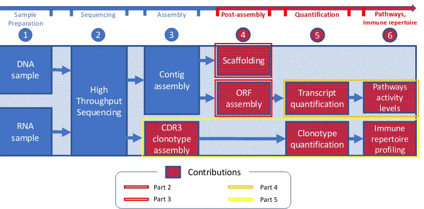
Figure 1.1 The bioinformatics pipeline for NGS data analysis. Compartments

drawn in red correspond to the main contributions of this dissertation.

Colored frames delimitate group of compartments corresponding to

different parts of this dissertation (for example, the main focus of Part

2 is scaffolding). . . 4

Figure 1.2 The structure of a mRNA transcript. Open reading frame is depicted

in green. . . 6

Figure 2.1 4 possibilities of connecting two contigs by a paired-end read [55]. 15

Figure 2.2 Gap estimation d is calculated in conformity with the formula: d = Lf−(L(A)−start(r1))−(L(B)−start(r2)), whereLf is the fragment

length, L(A), L(B) are lengths of contigs A and B, start(r1) (resp. start(r2)) is the distance from the starting position of r1 (resp. r2) to the beginning of the strand A (resp. B0). . . 19

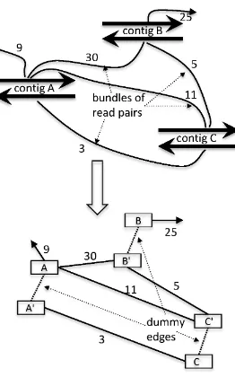
Figure 2.3 Contigs A, B, and C with connecting bundles of read pairs and the corresponding scaffolding graph. Each contig is split into two nodes

connected with a dummy edge. Each bundle of read pairs corresponds

to an inter-contig edge connecting respective strands with the weight

equal to the size of the bundle. A plausible scaffold corresponds to the

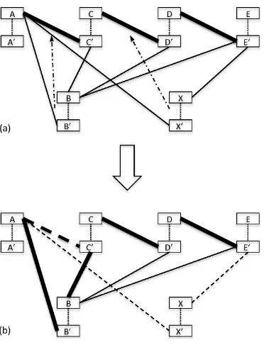
Figure 2.4 (a) A scaffoldA−B−C−D: the connection of each pair of adjacent contigs is supported by bundles of read pairs. (b) A path A0 −A−

B0 −B −C0 −C −D0 −D in the scaffolding graph corresponding to the scaffold A−B −C −D. (c) The matching of the scaffolding graph corresponding to the bunches of read pairs supporting adjacent

contigs. . . 22

Figure 2.5 Insertion procedure: (a) The matching scaffold A−C−D−E is ob-tained with the maximum weight matching; the contigB is connected with edges to all 4 contigs of the matching, the contig X is connected to A and C; B should be placed between A and C according to the consensus of connecting edges andX should be placed between C and D; (b) Since there is a sufficient distance between contigs A and C, B is placed there, i.e., the edge (A, C0) from the matching is replaced with (A, B0) and (B, C0) (the sum of weights of (A, B0) and (B, C0) is

less than the weight of (A, C0)); since there is no sufficient room forX between contigsC and D, the edges (A, X0) and (X, E0) are removed. The resulted scaffold is A−B−C−D. . . 24

Figure 2.6 Matching of contigs in the scaffolding S and in the referenceR. Only the links (2,3) and (4a,5) are mapped correctly. Contig 2 has two

copies 2a and 2b in the reference scaffolding, contig 4 is inferred to

have two copies 4a and 4b. Assigning contig 2 to either of the copy

2a or 2b, as well as assigning either 4a or 4b to the reference contig 4

affects the number of correctly inferred contigs links. Indeed, assigning

contig 2 to the reference contig 2a and contig 4b to 4 will mistakenly

undercount the number of correct links. The optimal assignment (2 to

Figure 2.7 The reference scaffolding contains three copies of contig 102 (namely,

102a, 102b, and 102c). In the reference scaffolding of Hunt et al. [40]

only the best hit is considered and two copies with a high identity

level (> 97%) are discarded. As a result the contig 102 is treated as

erroneously placed by SSPACE between contigs 19 and 20 resulting in

two false negative links. Similarly, since the contig 102c is missing, the

link between contigs 79 and 80 is falsely treated as correct. Finally,

the missing contig 102a is correctly classified. . . 34

Figure 2.8 Copy number distribution . . . 38

Figure 2.11 Classification of incorrect links. Contig 2 in the scaffolding output is

assigned to contig 2a in the reference, contig 4a in the scaffolding

out-put is assigned to contig 4 in the reference (marked with arrows). There

are two correct links (marked with green) and 4 wrong links (marked

with red). Link (6,1) connects contigs 6 and 1 coming from different

reference sequences. Link (2,3) connects contigs 2 and 3 which are

not in correct order/orientation. Jumping link (3,4a) connects

con-tigs 3 and 4a which are not in correct order/orientation. Link (5,4b)

connects contig 5 with an “extra” copy of contig 4 (namely 4b). . 43

Figure 2.12 Performance (F-score) of the scaffolding tools depends both on λ and α. The x axes of the heat maps denote the similarity level used to obtain the artificial contig datasets and the y axes of the heat maps denote the minimum length of contig in the dataset. This figure

dis-plays results for S. aureus. . . 46

Figure 2.13 (a) The scaffolding graphG. Each contig is represented by two vertices (+ and−) corresponding to forward and backward strands. The

intra-contig edges are dashed, the inter-intra-contig edges are solid. (b) The

scaffolding graph corresponding to a valid scaffold. The graph is a

chain of alternating intra- and inter-contig edges. (c) The chain of

contigs corresponding to the scaffolding graph of a scaffold. Each

contig is either in the original orientation (+) or inverted (−). . . 50

Figure 2.14 (a) A confusion triple: the same strand of contig A is connected with two strands of contigs B and C; The two possible scenarios causing the confusion: (b) The contig A is a repeat and another copy of contig

Figure 2.15 Insertion procedure. Contigs belonging to a backbone scaffold S have green color; contigs which are candidates for insertion have blue color.

a) A fragment of surrounding graph−G→S with the chain of trusted

con-tigs A, B, C and neighboring contigs X1 −X4. b) The directed sur-rounding graph−G→S corresponding toGS. c) The scaffoldS augmented

with contigs X1,X2, X3, and X4. . . 56

Figure 3.1 RNA-Seq data analysis flow. . . 63

Figure 3.2 Full ORF, 3’-partial (i.e. missing 3’-end), partial (i.e. missing

5’-end), and internal ORF. . . 64

Figure 3.3 A 3’-partial ORF has overlap of 9 nt with a 5’-partial ORF. . . . 67

Figure 3.4 (a) Red path with 6 hops; (b) Green path with 2 hops; (c) Yellow path

with 1 hop. . . 67

Figure 4.1 The pipeline MAP and the enhanced pipeline for quantification and

differential analysis of the metabolic pathway activity. The

quantifi-cation enhancements are drawn in red. . . 76

Figure 5.1 Overview of ImReP. (a) Schematic representation of human adaptive immune repertoire.

Adap-tive immune repertoire consists of four T cell receptor loci (blue color, T-cell receptor alpha locus

(TCRA); T-cell receptor beta locus (TCRB); T-cell receptor delta locus (TCRD); and T-cell

re-ceptor gamma locus (TCRG)) and three immunoglobulin loci (red color, Immunoglobulin heavy

locus (IGH); Immunoglobulin kappa locus (IGK) ; Immunoglobulin lambda locus (IGL).

Alter-native name – BCR, B cell receptor). B and T cell receptors contain multiple variable (V, green

color), diversity (D, present only in IGH, TCRB, TCRG, violet color), joining (J, yellow color)

and constant (C, blue color) gene segments. V(D)J gene segments are randomly jointed and

non-templated bases (N, dark red color) are inserted at the recombination junctions. The resulting

spliced T or B cell repertoire transcript incorporates the C segment and is translated into the

antigen receptor proteins. RNA-Seq reads are derived from the rearranged immunoglobulin IG

and TCR loci. Reads entirely aligned to genes of B and T cell receptors are inferred from mapped

reads (black color). Reads with extensive somatic hypermutations and reads spanning the V(D)J

recombination are inferred from the unmapped reads (grey color). Complementarity determining

region 3 (CDR3) is the most variable region of the three CDR regions and is used to identify

T/B cell receptor clonotypes—a group of clones with identical CDR3 amino acid sequences. (b)

Receptor derived reads spanning V(D)J recombinations are identified from unmapped reads and

assembled into the CDR3 sequences. We first scan the amino acid sequences of the read and

determine the putative CDR3 boundaries defined by last conserved cysteine encoded by the V

gene and the conserved phenylalanine (for TCR) or tryptophan (for BCR) of J gene. Given the

putative CDR3 boundaries, we check the prefix and suffix of the read to match the suffix of V

and prefix of J genes, respectively. (c-d) In case a read overlaps with only the V or J gene, we

perform the second stage of ImReP to match such reads based on the overlap of CDR3 sequence

using suffix tree. We map D genes (for IGH, TCRB, TCRG) onto assembled CDR3 sequences

and infer corresponding V(D)J recombination. . . 94 Figure 5.2 ImReP vs MiXCR on simulated data: recall plots for coverages 1, 2,

4, 8, 16, 32, 64, 128: a) Read length 50 bp; b) Read length 75 bp; c)

Figure 5.3 ImReP vs MiXCR on simulated data: precision plots for coverages 1,

2, 4, 8, 16, 32, 64, 128: a) Read length 50 bp; b) Read length 75 bp;

c) Read length 100 bp. . . 96

Figure 5.4 Diversity of adaptive immune repertoire across multiple human tissues. Heatmaps

LIST OF ABBREVIATIONS

• ORF - Open Reading Frame

• PPV - Positive Predictive Value

• TPR - True Positive Rate

• ILP - Integer Linear Programming

• BCR - B Cell Receptor

• TCR - T Cell Receptor

• NGS - Next Generation Sequencing

• HTS - High Throughput Sequencing

• CDR3 - Complementarity-Determining Region 3

• EM - Expectation Maximization

PART 1

INTRODUCTION

One of the most important and challenging biological tasks has been discovery and deciphering of the human genetic code [17]. To understand the process of life, one needs to determine the sequence of the four bases - adenine, guanine, cytosine, and thymine (A, G, C, T) which make up the human genome. One of the earliest technologies for DNA sequencing is so-called Sanger sequencing [78] based on specific chain-terminating inhibitors of DNA polymerase. Its main advantage is very low error rate [92], but it is not practical due to its high costs. Thus, The Human Genome Project (HGP), used a newer technology of shotgun sequencing (i.e. shearing DNA into multiple random pieces and then assembling into the genome sequence) which is considerably cheaper than the Sanger sequencing but poses challenging computational problems requiring a lot of resources.

A new era in life sciences has begun with the advent of the Next Generation Sequencing (NGS) technologies: 454, Illumina, SOLiD, Ion Torrent. These new technologies revolution-ized the field of bio- and medical sciences, in particularly, bioinformatics, as they allowed generating millions of high quality reads (single- and paired-end) with a significant drop of cost per base pair. The new technologies posed new problems, but at the same time, they allowed expanding the range of bioinformatics applications which can leverage the massive data produced by them: variant calling, discovery of germline and somatic mutations, etc.

pathways which represent networks of biochemical reactions.

As the Central Dogma [16] of molecular biology assumes the informational flow from DNA to proteins, most of the bioinformatics pipelines start with analyzing NGS reads and end up with downstream analysis like differential gene expression or estimation of biological pathway activity. This dissertation presents multiple algorithmic contributions on all three informational levels of the Central Dogma unified into one bioinformatics pipeline for NGS data analysis.

1.1 Background

In this section, we provide the description of most widely spread Next Generation Se-quencing technologies and importance of their multiple applications and also highlight the structure of the bioinformatics pipeline which serves as the skeleton unifying the contribu-tions of this dissertation.

1.1.1 NGS technologies

The importance of Next Generation Sequencing technologies cannot be underestimated because they allow for rapid advances in life sciences. They are used in a very large set of applications, the most important of which are [35]:

• Resequencing of human genome for discovery of genes and regulatory elements involved in different diseases;

• Comparative biology studies through whole-genome sequencing of multiple species;

• Sequencing of bacterial and virus species for public health and epidemiological studies;

• Gene expression studies through RNA-Seq technologies etc.

Table 1.1 NGS technologies and their characteristics [13].

Sequencing Platform Sequence

by Run types Run time Read length Reads per run Output per run Roche GS FLX

Titanum XL+ Synthesis Single end 23h 700 1 M 700 Mb

GS Junior

System Synthesis Single end 10 h 400 0.1 M 40 Mb

Life-Technologies

Ion Torrent Synthesis Single end 4h 200-400 4 M 1.5-2 Gb

Proton Synthesis Single end 4h 125 60-80 M 8-10 Gb

Abi/solid Ligation Single end &

paired-end 10d 75 + 35 2.7 B 300 Gb

Illumina HiSeq Synthesis

Single end &

paired-end 12d 2 x 100 3 B 600 Gb

MiSeq Synthesis Single end &

paired-end 65h 2 x 300 25 M 15 Gb

PacBio RSII Single molecule

synthesis Single end 2d 10 K 0.8 M 5 Gb

Helicos Heliscope Single molecule

synthesis Single end 10d 30 500 M 15 Gb

To analyze the massive datasets produced by NGS platforms researchers have to design specialized pipelines for processing raw reads and getting particular bioinformatics results. In this dissertation, the main focus is on the pipeline which leads from NGS reads to biological pathways.

1.1.2 Bioinformatics Pipeline for NGS Data Analysis

Pathways, Immune repertoire High Throughput Sequencing Contig assembly DNA sample RNA sample CDR3 clonotype assembly ORF assembly Immune repertoire profiling Pathways activity levels Scaffolding Upstream Downstream Sample Preparation

Sequencing Assembly Post-assembly Quantification

Transcript quantification

Clonotype quantification

1 2 3 4 5 6

Part 2 Part 3

Part 4 Part 5

Contributions

Figure 1.1 The bioinformatics pipeline for NGS data analysis. Compartments drawn in red correspond to the main contributions of this dissertation. Colored frames delimitate group of compartments corresponding to different parts of this dissertation (for example, the main focus of Part 2 is scaffolding).

1-3 described above are referred to as upstream analyses and are well studied.

Next three stages referred to as downstream analyses constitute the core of this disser-tation. In the stage 4 (post-assembly), DNA contigs are joined into chains where each contig is ordered and oriented. This process is referred to as scaffolding. Also, RNA sequences corresponding to transcripts without a full open reading frame (ORF) are assembled further to contain a full ORF coding for a protein. In the stage 5, transcripts and CDR3 clono-types are undergone a quantification analysis. In this step, the relative abundance for each transcript/clonotype is determined. In the utmost stage of our pipeline, stage 6, further downstream analyses are performed (such as pathways activity levels or immune repertoire profiling).

1.2 Problems

Scaffolding Problem. Next Generation Sequencing (NGS) technologies (Illumina, Ion Tor-rent) produce reads that are several hundreds of nucleotide base pairs long. It is challenging to assemble genomes due to some drawbacks which are still characteristic of these tech-nologies: uneven read coverage, sequencing errors, insufficient read length to span repeated regions in genomes. All these issues hinder the genome assembly problem to be solvable in polynomial time. Thus, overcoming technological issues to allow for better assemblies of dif-ferent species is still crucial. Several attempts are being made by so-called Third Generation Sequencing technologies (Pacific Biosciences, Oxford Nanopore Technologies) to increase the read length up to several thousand base pairs, but currently they have a very high error rate (≈15% for Pacific Biosciences) compared to NGS (Illumina MiSeq<1%) and they are still

under active development. Therefore, there is still a high demand for developing efficient and scalable assembly algorithms for the genome assembly problem.

Genome assembly pipeline has been traditionally divided into three main stages: as-sembly, scaffolding, and gap filling. The output of the assembly stage is the set of contiguous DNA sequences called contigs. Contig length depends on the assembly tool and the other factors mentioned previously (read length, uniformity of coverage, etc). The set of contigs and the paired-end reads serve as input to the scaffolding stage. The main goal is to join contigs into chains called scaffolds to correctly determine the relative orientation, the rela-tive ordering, and the distance between adjacent contigs in each scaffold. So the scaffolding problem in general case can be formulated as follows:

Scaffolding Problem. GivenC - the set of contigs andP - the set of paired-end reads, build a set of scaffolds S maximizing the optimization criterion K.

Here K may, for example, be the number of correct contig joins. The last stage of genome assembly is gap filling. Here the gaps remaining after the previous step are closed using the reads.

(see Figure 1.2). The ORF is the most interesting and important transcript part from the biological perspective since it potentially codes for a protein. It begins with a start codon Met (methionine, AUG nucleotide sequence) and ends with a stop codon (either UAA, or UAG, or UGA). State-of-the-art RNA-Seq assemblers like Trinity [34] often output transcripts which do not contain the full ORF and are either missing the 5’-prime, 3’-prime or both ends. The portion of such non-complete transcripts may be considerable resulting in losing much of the information contained in an RNA-Seq sample. The problem of ORF assembly is about having a set of non-complete ORFs extracted from a set of transcripts to join them into as many as possible full ORFs.

Open Reading Frame 3’UTR

5’ UTR Poly-A

tail Cap

Start End

5’

3

’

Figure 1.2 The structure of a mRNA transcript. Open reading frame is depicted in green.

Gene and Isoform Quantification. Estimating gene and isoform expression levels is a very important bioinformatics problem. Due to recent advances in sequencing technologies, millions of paired-end high-quality RNA-Seq reads can be produced in a usual experiment. The amount of data and the intrinsic properties of transcriptomes (e.g. human) make it a very challenging task. In general, quantification methods are divided into two main cat-egories: count-based (e.g. HTSeq [3]) and FPKM-based (e.g. IsoEM [68], RSEM [51]). Although FPKM-based methods are deemed to usually outperform count-based methods [43] in terms of accuracy, the ultimate goal of any RNA-Seq experiment is to estimate differ-ential gene and/or isoform expression levels. The problem becomes even harder in absence of enough number of replicates.

amount of these enzymes participating in biochemical reactions. As a result, if some enzymes are overrepresented/underrepresented the corresponding reactions occur with more/less in-tensity, i.e. the activity level of the corresponding pathways increases/decreases. Therefore, in this context, a problem of inference of pathway activity levels from RNA-Seq reads is formulated. One of the main challenges of this problem is the fact that many enzymes work in the context of several pathways, thus creating ambiguities of assignment.

CDR3 Sequence Assembly. The adaptive immune system is a very important biological mechanism which eliminates and prevents the growth of pathogens in the host organism. The immune response is carried out by the two main cell types - B cells and T cells. They secrete antibodies known as immunoglobulins. The part of the antibody known to serve as a binding site to antigenes is highly variable and is called Complementary Determining Region 3 (CDR3). The hypermutations and the genetic V(D)J recombination between the V, D, and J genomic segments can code for a virtually unbounded number of antobody types. Due to this fact, assembling the whole immune repertoire from a set of RNA-Seq reads is a challenging task. The assembled CDR3 sequences are usually clustered into so-called clonotypes. For a comprehensive immune repertoire profiling one also needs to quantify the relative abundance of each clonotype.

1.3 Contributions

• A novel stand-alone scaffolding algorithm ScaffMatch which is based on the

repre-sentation of the scaffolding problem as the Maximum Weight Acyclic 2-Matching. This approach allows to efficiently use the intrinsic DNA properties (such as self-complementarity) to formulate and solve the scaffolding problem in a reasonable amount of time even for whole genome-scale datasets. Approximate solutions of Max-imum Weight Acyclic 2-Matching problem are found using a heuristic based on Maxi-mum Weight Matching which is known to be solvable in polynomial time.

repeated contig sequences. It allows to adequately measure the quality of scaffolding assemblies produced by the current state-of-the-art tools as well as the tools adjusted to handle repeats.

• Releasing a novel repeat-aware scaffolding tool called BATISCAF which performs an

optimal spurious contig filtering resulting in the scaffolding problem to be reduced to a trivial case. Contigs which are repeated are re-inserted into scaffolding as many times as it can be inferred from the scaffolding graph structure.

• Development of ImReP, a novel computational method for rapid and accurate profiling of adaptive immune repertoire from RNA-Seq data. ImReP can efficiently extract TCR- and BCR- derived reads from the RNA-Seq data and assemble corresponding B and T cell receptor clonotypes.

• A novel tool DORFA for protein database guided ORF (open reading frame) assembly.

It takes as input the set of partial ORFs produced by an RNA-Seq assembler and builds from them complete ORFs. The biological value of our tool is very important since it complements the output of a de-novo RNA-Seq assembler. Finding the exhaustive set of ORFs can be crucial for accurate protein activity level estimation or for pathway reconstruction.

• New release of the IsoEM2/IsoDE2 suite for RNA-Seq gene and isoform expression

level estimation and differential expression analysis. The main feature of these tools is the fast non-parametric computation of confidence intervals and identification of DE genes based on bootstrapping.

• A novel tool EMPathways for inference of pathways activity levels from RNA-Seq data

1.4 Roadmap

This dissertation is organized as follows. Chapter 1 presents a highlight of the Next Gen-eration Sequencing Technologies and gives a global overview of the algorithms and methods in the context of the bioinformatics pipeline described in Section 1.1.2.

In the following chapters, novel and efficient algorithms related to different parts of the pipeline are presented. In particular, Chapter 2 presents a novel scaffolding algorithm ScaffMatch which outperforms many of the existing approaches. A conceptually new method-ology for scaffolding quality assessment is proposed. Finally, a novel repeat-aware scaffolding tool BATISCAF is described. The main focus here is on the first level of the Central dogma flow. Chapter 3 proposes an assembly algorithms at the second level of the Central dogma. Namely, DORFA is designed to assemble open reading frames (ORFs) from partial RNA-Seq contigs. Chapter 4 mainly being at the third level of the Central dogma proposes a maxi-mum likelihood approach for inferring pathways activity levels from RNA-Seq data. Along with this, a differential bootstrap based statistical approach for inferring significant up- and down-regulated pathways is presented. Chapter 5 is completely dedicated to the immune profiling part of the pipeline. The new method for CDR3 sequence assembly and immune profiling called ImReP is proposed.

1.5 Scientific Products

1.5.1 Publications

• Book Chapters

1. Igor Mandric, James Lindsay, Ion M˘andoiu, Alex Zelikovsky “Scaffolding Algo-rithms” Computational Methods for Next Generation Sequencing Data Analysis, 2016.

1. Igor Mandricand Alex Zelikovsky. “Solving scaffolding problem with repeats”. Bioinformatics (Submitted).

2. Igor Mandric, Sergey Knyazev, and Alex Zelikovsky. “Repeat aware evaluation of scaffolding tools”. Bioinformatics (2018).

3. Pavel Skums, Alex Zelikovsky, Rahul Singh, Walker Gussler, Zoya Dimitrova, Sergey Knyazev, Igor Mandric, Sumathi Ramachandran, David Campo, Deep-tanshu Jha, Leonid Bunimovich, Elizabeth Costenbader, Connie Sexton, Siobhan O’Connor, Guo-liang Xia, Yury Khudyakov. “QUENTIN: reconstruction of dis-ease transmissions from viral quasispecies genomic data”. Bioinformatics (2017) 34 (1): 163-170.

4. Igor Mandric, Yvette Temate-Tiagueu, Tatiana Shcheglova, Sahar Al Seesi, Alex Zelikovsky, Ion M˘andoiu. “Fast bootstrapping-based estimation of con-fidence intervals of expression levels and differential expression from RNA-Seq data”. Bioinformatics (2017) 33 (20): 3302-3304.

5. Serghei Mangul, Igor Mandric, Harry Taegyun Yang, Nicolas Strauli, Dennis Montoya, Jeremy Rotman, Will Van Der Wey, Jiem R Ronas, Benjamin Statz, Alex Zelikovsky, Roberto Spreafico, Sagiv Shifman, Noah Zaitlen, Maura Rossetti, K Mark Ansel, Eleazar Eskin. “Profiling adaptive immune repertoires across multiple human tissues by RNA Sequencing”. bioRxiv2017.

6. Yvette Temate-Tiagueu, Sahar Al Seesi, Meril Mathew, Igor Mandric, Alex Rodriguez, Kayla Bean, Qiong Cheng, Olga Glebova, Ion M˘andoiu, Nicole B Lopanik, Alexander Zelikovsky. “Inferring metabolic pathway activity levels from RNA-Seq data”. BMC Genomics 2016 17(Suppl 5):542.

7. Igor Mandric and Alex Zelikovsky. “ScaffMatch: scaffolding algorithm based on maximum weight matching”. Bioinformatics (2015) 31 (16): 2632-2638.

1. Igor Mandric, James Lindsay, Ion M˘andoiu, Alex Zelikovsky. ‘SILP3: Maxi-mum likelihood approach to scaffolding‘. IEEE 4th International Conference on Computational Advances in Bio and Medical Sciences (ICCABS) (2014)

2. Yvette Temate-Tiagueu, Meril Mathew,Igor Mandric, Qiong Cheng, Olga Gle-bova, Nicole Beth Lopanik, Ion M˘andoiu, Alex Zelikovsky. “Metabolic path-way activity estimation from RNA-Seq data”. 11th International Symposium on Bioinformatics Research and Applications (ISBRA) (2015).

3. Igor Mandric, Sergey Knyazev, Cory Padilla, Frank Stewart, Ion M˘andoiu, Alex Zelikovsky. “Metabolic Analysis of Metatranscriptomic Data from Planktonic Communities”. 13th International Symposium on Bioinformatics Research and Applications (ISBRA) (2017).

4. Igor Mandric and Alex Zelikovsky. “ScaffMatch: scaffolding algorithm based on maximum weight matching”. Research in Computational Molecular Biology (RECOMB) 2015.

• Conference Abstracts

1. Igor Mandric, Yvette Temate-Tiagueu, Adrian Senatore, Paul Katz, and Alex Zelikovsky. “DORFA: Database-guided ORFeome assembly from RNA-Seq data”. IEEE 5th International Conference on Computational Advances in Bio and Med-ical Sciences (ICCABS) (2015).

1.5.2 Presentations

2. Igor Mandric, Sergey Knyazev, and Alex Zelikovsky. “Repeat aware evaluation of scaffolding tools”. The 7th RECOMB Satellite Workshop on Massively Parallel Sequencing (RECOMB-Seq) (2017).

3. Serghei Mangul, Igor Mandric, Alex Zelikovsky and Eleazar Eskin. “Profiling adaptive immune repertoires across multiple human tissues by RNA Sequenc-ing”. The 21st Annual International Conference on Research in Computational Molecular Biology (RECOMB) (2017).

4. Igor Mandric and Alex Zelikovsky. “BATISCAF: solving scaffolding problem with repeats”. The 8th RECOMB Satellite Workshop on Massively Parallel Se-quencing (RECOMB-Seq) (2018)

1.5.3 Software Packages

• ScaffMatch - Scaffolding by Maximum Weight Matching. https://github.com/

mandricigor/ScaffMatch.

• IsoEM2 - Inferring Gene and Isoform Expression through Expectation-Maximization.

https://github.com/mandricigor/isoem2.

• DORFA - Database-guided ORFeome Assembly. https://github.com/mandricigor/

DORFA.

• ImReP - Profiling Immune Repertoire from RNA-Seq data. https://github.com/

mandricigor/imrep.

• EMPathways - Estimation of Pathways activity levels from RNA-Seq data. https:

//github.com/mandricigor/EMPathways.

• BATISCAF - BAd conTIg filtering SCAFfolding. https://github.com/

mandricigor/batiscaf.

• Repeat-aware evaluation framework. - https://github.com/mandricigor/

PART 2

ALGORITHMS FOR SCAFFOLDING AND SCAFFOLDING EVALUATION

2.1 Introduction

Due to rapid advances in High-Throughput Sequencing (HTS) technologies the interest in the problem ofde novogenome assembly has been renewed. These powerful technologies, also referred to as Next-Generation Sequencing (NGS), can produce millions of short paired-end reads covering whole genome; thus, the throughput is a magnitude higher than the classic Sanger sequencing. It is worth noticing that the cost of producing reads keeps a trend of decreasing making NGS a very attractive tool for a high range of applications. For example, Illumina HiSeq platform is able to produce billions of read pairs in a single run at a cost of cents per megabase. Although the number of reads (shotgunreads) is significant, due to their short length, genome assembly still represents a challenging problem. Assembled genomes are frequently highly fragmented and consist of contigs of highly variable length. The connectivity information coming from read pairs mapped to contigs can be used to merge them into ascaffoldwhich is a set of chains of oriented ordered contigs with estimated gaps between all pairs of adjacent elements.

the estimation of the gap length between neighboring contigs is provided, is called scaffold. Software programs, usually referred to asscaffolders, construct scaffolds based on contigs output by an assembler and the connectivity information provided by the NGS read pairs. Due to misassemblies in contigs, repeats and chimeric reads, the information about relative ordering and orientation of two contigs connected with a set of read pairs can be contradictory and not reliable. Thus, choosing a wrong subset of read pairs as an evidence for a connection between two contigs, can result in inferring a wrong relative ordering and/or orientation as well as the gap estimation between them. Edges that comply with the true orientation of contigs and the distance between them are usually called concordant, otherwise discordant edges.

In [30] it is proven that the Scaffolding Problem is an NP-hard problem. Thus, all state-of-the-art scaffolders use different heuristic approaches. A recent comprehensive evaluation of available software tools has shown that the scaffolding problem still does not have an adequate solution [40]. This means that most of the available scaffolders are not able to optimally (or at least close to an optimal solution) solve the scaffolding problem and there is still a lot of room for further improvements. In this subsection, a brief overview of the most important scaffolding tools is provided.

(A)

5’ 3’ 5’ 3’

R3 F3

CONTIGi CONTIGj

5’ 3’ 5’

F3 R3

CONTIGi CONTIGj 3’

5’ 3’ 5’ 3’

R3 F3

CONTIGi CONTIGj 5’ 3’ 5’

F3 R3

CONTIGi CONTIGj 3’ (B)

(C)

5’ 3’ 5’ 3’

R3 F3

CONTIGi CONTIGj

5’ 3’ 5’

F3 R3

CONTIGi CONTIGj 3’

5’ 3’ 5’ 3’

R3 F3

CONTIGi CONTIGj 5’ 3’ 5’

F3 R3

CONTIGi CONTIGj 3’ (D)

Figure 2.1 4 possibilities of connecting two contigs by a paired-end read [55].

OPERA implements an elegant dynamic programming scaffolding algorithm that solves the Scaffolding Problem of maximizing the number of concordant edges in the scaffold. SOPRA (Scaffolding algorithm for paired reads via statistical optimization) [18] solves the Scaffolding Problem by using methods inspired from statistical physics. The SOPRA algorithm consists of several stages. In the first stage, the problem of contig orientation is solved. For a pair of contigs i and j a value Jij is introduced, which is equal to the signed number of contigs

supporting a certain relative orientation. The sign ofJij depends on the orientations of the

contigs iand j: if they have the same orientation, then the sign of Jij is positive, otherwise,

it is negative. SOPRA searches such a configuration of the contigs, that minimizes the sum

− X

(i,j)∈E(G)

JijSiSj,

where Si ∈ {−1,+1}stands for the contig orientation.

SILP2 [55] and its improved version SILP3 [60] propose an Integer Linear Programming (ILP) formulation based on the four possibilities of a paired read to join two contigs (See Figure2.1).

The flow of SILP3 (further, we will refer only to SILP3) consists of the following steps (which are very similar to many other tools):

1. mapping reads onto contigs

2. scaffolding graph construction

3. maximum likelihood contig orientation via ILP

4. decomposition into paths of orientation compatible edges via bipartite matching

5. maximum likelihood gap estimation

The scaffolding graphG= (V, E) is constructed as to connect the vertices-contigs with the edges-read pairs. Maximum likelihood contig orientation is formulated as the following ILP [55]. Let Si be a boolean variable with value being set to 0 if the orientation of contig i remains unchanged. The 4 states A, B, C, D (Figure 2.1) in which a pair (i, j) of contigs can be based on their orientation and relative ordering. The 4 boolean variables Aij, Bij, Cij, Dij ={0,1} ∀(i, j) correspond to the 4 states. For each state a weightAijw, Bijw,Cijw, Dijw

using a maximum likelihood approach is calculated. The number of concordant contig pairs is then maximized:

M ax X

(i,j)∈E

Aw_ij ·Aij +Bijw·Bij +Cijw·Cij+Dwij ·Dij

subject to constraints connecting Aij, Bij, Cij, Dij with Si. SILP3 applies the technique

of non-serial dynamic programming [82] in order to solve the optimization problem. The output of this step is a directed graph G0 = (V, E0, w, g) in which each contig and each edge has the most likely orientation, w : E0 → R+ _{is the weight of an edge contributing to the}

AnorderingO is a graph consisting of a set of disjoint directed chains of contigs together with estimations of gaps between all pairs of adjacent contigs. Note that in the ordering O

the estimation of gaps between adjacent contigs uniquely defines the gapgO(i, j) between any

pair of connected contigsi and j. SILP2 [55] extracts the maximum subgraph-ordering out of G0. Instead, SILP3 is aimed to find an ordering with the maximum support of G0-edges. A directed edgee= (i, j)∈E0 isconcordant with an orderingO if iprecedes j inO and the gap|g(e)−gO(i)| ≤5σ, where σis the standard deviation of read pair fragment length. The

maximum likelihood ordering is approximated with the ordering concordant with the edges of G0 of the maximum total w-weight.

SILP3 first runs depth-first search (DFS) on G0 recursively deleting least-weight edge resulting in G0 being a directed acyclic graph (DAG). Any topological order of G0 is order-concordant with all edges remaining in G0. Let C be the set of contigs between i and j in

G0. C is sorted based on their distance estimations to i and j, Csorted ={i1, i2, ..., ik}. All

edges in the graph are replaced with the directed path P0 ={i, i1, i2, ..., ik, j}. Then SILP3

determines the maximum weight bipartite matching similar to SILP2.

Contributions. In this chapter, a novel scaffolding algorithm called ScaffMatch [62] will be presented in details. Its main advantage over all other existing algorithms is that it formulates the Scaffolding Problem as a combinatorial optimization problem of finding the maximum-weight acyclic 2-matching problem (in other words, a subset of edges of the graph such that each vertex has degree at most 2). With a suitable reduction to the maximum weight matching problem, the almost optimal scaffolding can be determined in polynomial time (O(n3_{)). By using the greedy heuristic, ScaffMatch is able to solve the Scaffolding}

Problem in linear time. As multiple experimental results show, ScaffMatch outperforms most of the standard state-of-the-art scaffolding tools.

hinder significantly the process of evaluation of scaffolding results. A novel repeat aware evaluation framework is presented in this chapter. Its advantage is that it is able to compare scaffolding results making abstraction of whether repeats are handled by the scaffolding tool or not. Also, it provides insight into scaffolding results by making a comprehensive classification of incorrect joins. This can leverage further research in genome scaffolding.

Not of less importance is the contribution which relates to repeat aware scaffolding. In this thesis, a novel repeat aware tool called BATISCAF is presented. BATISCAF tackles the scaffolding problem differently than all previous tools. Namely, it is focused not on finding paths corresponding to scaffolds (as most of the tools do) but on an optimal spurious contig filtering. The two types of spurious contigs complicating the task of scaffolding are (i) short (ii) repeated contigs. By eliminating them from the scaffolding graph BATISCAF reduces the computationally hard problem to a trivial case. Afterward, the previously filtered contigs are re-inserted back into the scaffolds by using a maximum likelihood approach. The repeated contigs may be re-inserted multiple times (as many times as it can be inferred by the algorithm from the scaffolding graph structure).

2.2 ScaffMatch: combinatorial optimization approach to genome scaffolding

We proposed a novel optimization formulation representing scaffolding as a maximum-weight acyclic 2-matching problem. Since the Hamiltonian path problem can be reduced to this problem, this formulation is also NP-complete. The presented algorithm ScaffMatch efficiently finds the maximum-weight 2-matching and iteratively destroys all cycles. This approach works very well since, usually, number of cycles is very small.

follow-ing [40]. Our matching-based tool ScaffMatch compares favorably with the state-of-the-art tools in terms of the widely accepted N50 metric, the metrics introduced in [40], as well as sensitivity, PPV (positive predictive value), and F-score in predicting contig junctions.

Figure 2.2 Gap estimationd is calculated in conformity with the formula: d=Lf−(L(A)− start(r1))−(L(B)−start(r2)), where Lf is the fragment length, L(A), L(B) are lengths of

contigs A and B, start(r1) (resp. start(r2)) is the distance from the starting position of r1

(resp. r2) to the beginning of the strand A (resp. B0).

Methods. Below we describe the problem formulation and algorithmic details in the fol-lowing main scaffolding steps:

• Preprocessing of read pairs including read mapping, handling repeats and gap

estima-tion for each read pair.

• Scaffolding graph construction with vertices corresponding to contig strands and edges corresponding to read pairs.

• Matching scaffold finding near-maximum weight paths in the scaffolding graph and the

corresponding orientation and ordering contigs.

• Insertion of skipped contigs into the matching scaffold.

We conclude with the implementation details of ScaffMatch.

2.5σ than the average whereσ is the standard deviation of contig coverage. This empirically chosen threshold allows to remove the majority of repeats while keeping almost 99% of correct contigs. Although assemblers may give chimeric contigs or produce two contigs for the same genomic region (representing the two haplotypes) ScaffMatch does not attempt to identify or modify any contigs.

Each read is mapped only to one of the two contig strands (palindromes are discarded). For each read pair connecting two distinct contig strands, we estimate the gap according to Figure 2.2 (for an alternative gap estimation model see [73]). Among all read pairs connecting the same contig strands, we find a read pair p with the median gap estimation and then bundle p with all read pairs whose gap estimation is at most 3σ away from p’s estimation. Since we want to keep only reads that agree with each other, the reads outside of this bundle are discarded.

Scaffolding graph. Each vertex of the scaffolding graphG= (V, E) corresponds to one of the contig strands and eachinter-contigedge corresponds to a bundle of read pairs connecting two strands of different contigs (see Figure2.3). The weight of an inter-contig edge is equal to the size of the corresponding bundle. Also for each contig, we have adummyedge connecting its two strands.

Matching Scaffolding. Ideally, we expect that the scaffolding graph would consist of a set of paths each corresponding to a different chromosome (see Figure 2.4(a)). Unfortunately, repeats introduce noisy edges connecting unrelated contigs even from different chromosomes. Additionally, the paths corresponding to chromosomes may skip short contigs (especially contigs which are shorter than the insert length). Therefore, any set of paths passing through all dummy edges in the scaffolding graph G corresponds to a plausible scaffold (see Figure

2.4(b)). The most likely scaffold would be supported by the largest number of read pairs. Therefore, we can formulate the following

Figure 2.3 ContigsA,B, andC with connecting bundles of read pairs and the corresponding scaffolding graph. Each contig is split into two nodes connected with a dummy edge. Each bundle of read pairs corresponds to an inter-contig edge connecting respective strands with the weight equal to the size of the bundle. A plausible scaffold corresponds to the path

C0−C−A0−A−B0 −B supported by two inter-contig edgesCA0 and AB0.

By setting the weight of each dummy edge to a large number (e.g., number of all read pairs), we reduce the scaffolding problem to the following

Maximum-Weight Acyclic 2-Matching (MWA2M) Problem. Given a weighted graph G = (V, E, w), find a maximum weight acyclic subset of edges

M ⊆E such that each vertex v ∈V is incident to at most 2 edges inM.

The MW2AM of an n-vertex graph G with all edge weights 1 has the weight n−1 if and only if G has a Hamiltonian path. Therefore, the MWA2M problem is NP-complete since it includes the Hamiltonian path problem. A similar well-known problem, the Maximum Weight 2-Matching (MW2M), allows chosen edges to form cycles. In contrast to the MWA2M problem, the MW2M problem can be efficiently solved [70].

Figure 2.4 (a) A scaffold A−B−C−D: the connection of each pair of adjacent contigs is supported by bundles of read pairs. (b) A path A0 −A−B0 −B −C0−C−D0 −D in the scaffolding graph corresponding to the scaffold A−B−C−D. (c) The matching of the scaffolding graph corresponding to the bunches of read pairs supporting adjacent contigs.

weighted graphs. It starts with finding the maximum-weight matching M among the inter-contig edges. All the dummy edges also form a matching D. If the union of these two matchings M ∪D does not contain cycles, then the heuristic reaches the optimal collection of paths. Otherwise, a negative weight −1 is assigned to the least weight inter-contig edge in each cycle. The above steps of finding the inter-contig matching M and destroying cycles inM ∪D are repeated until the unionM ∪D becomes a collection of paths. The output of this heuristic will be called the Matching Scaffold.

In general, the deletion of least-weight edges may significantly reduce (as much as twice in the worst case) the total weight of the collection of paths. Fortunately, the erroneous heavy inter-contig edges are very rare in real data. Our experiments show that for each scaffolding example there is no more than a single cycle in the initial union M ∪D of the maximum-weight matchingM and the dummy edges solution and after the second iteration,

M ∪D does not contain any cycles at all.

decreased using the Greedy Heuristic repeatedly choosing the heaviest feasible edge, i.e., an edge which does not make a vertex degree higher than 2 and does not form cycles with the previously chosen edges. Note that the Greedy Heuristic picks the globally heaviest edge in contrast to greedy scaffolders (such as SSPACE) greedily extending existing chains. We provide an option that allows ScaffMatch to run with the Greedy Heuristic reducing the run-time complexity fromO(n3) to O(n·log n) as we use max heap in our implementation. Our experiments show that the Greedy Matching performs very well in practice but sacrificing not much in quality to the Maximum-Weight Matching heuristic.

Contig ordering and orientation. The Matching Scaffold is represented by a collection of disjoint chains of contig strands. The sequence of edges along each chain alternates: two strands of the same contig are connected with a dummy edge, two strands of different contigs are connected with an inter-contig edge. When traversing the strands along the paths in the matching scaffold, the order of traversing ends of dummy edges gives us the orientation of the corresponding contigs and the order of traversing inter-contig edges gives us the relative order of contigs.

Insertion of skipped contigs. The Matching Scaffold can skip short contigs whose length is less than the read pair insert size. For example, let the true scaffold contain a triple of consecutive contigs A, B and C such that lA > lins, lC > lins, but lB lins. Then instead

of picking both edges AB and BC, the Matching Scaffold may choose one single edge AC

since the edge weight between short contigs depends almost linearly on the length of the contigs. Thus, even though the contig B must follow A in the final scaffold, the weight of the edge between A and B is much smaller than the weight of the edge between A and C, which “jumps” over B.

to the same slot, their relative order and orientation is decided based on the gap estimations as follows. For each skipped contig (X0, X), we estimate the distance to the left contig and orient it according to the adjacent strands. Then we sort all contigs with respect to this distance and insert them according to this order.

Figure 2.5 Insertion procedure: (a) The matching scaffold A−C−D−E is obtained with the maximum weight matching; the contig B is connected with edges to all 4 contigs of the matching, the contig X is connected to A and C; B should be placed between A and C

according to the consensus of connecting edges and X should be placed between C and D; (b) Since there is a sufficient distance between contigs A and C, B is placed there, i.e., the edge (A, C0) from the matching is replaced with (A, B0) and (B, C0) (the sum of weights of (A, B0) and (B, C0) is less than the weight of (A, C0)); since there is no sufficient room for X

between contigsC and D, the edges (A, X0) and (X, E0) are removed. The resulted scaffold is A−B−C−D.

Algorithm 1 Insertion of skipped contigs

1: SLOT S ← {}

2: SKIP P ED ←the set of skipped contigs

3: M ={m1, m2, ..., mn} ← the Matching Scaffold 4: G= (V, E, w)← the Scaffolding Graph

5: l← insert length

6: for all X = (X0, X)∈SKIP P ED do

7: for all m ∈M do

8: if ∃ contigs A = (A, A0), B= (B, B0)∈m

s.t. (A, X0)∈E and (B0, X)∈E &

gap(A,X) +l(X) +gap(X,B)≤l then

9: for each edgee= (Ci,Ci+1)∈m(A,B)do

10: if gap(A,Ci)≤gap(A,X) and gap(Ci+1,B)≤gap(X,B) then

11: SLOT S[e,X] += w(A, X0) +w(X, B0)

12: end if

13: end for

14: end if

15: end for

16: end for

17: for all X ∈SKIP P ED do

18: e ←max{SLOT S[e,X]|e∈E}

19: insert X into e 20: end for

21: return SLOT S

the paired-end reads. The program outputs a fasta file with scaffolds. We use Networkx python library for graph computations [38].

2.2.1 Results

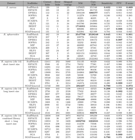
Datasets. We validate and compare the scaffolding tools on the collection of scaffolding datasets used in [40] including 4 datasets from the GAGE project [76] (Staphylococcus aureus, Rhodobacter sphaeroides andHomo sapiens (chr14)) and one additional datasetPlasmodium falciparum following [40]. All contigs were assembled by Velvet [100]. The Table 2.9 gives the parameters of all used scaffolding datasets.

Table 2.1 Scaffolding Datasets

Datasets insert size read length # contigs # reads

S. aureus 3600 37 170 3494070

R. sphaeroides 3700 101 577 2050868

H. sapiens (chr14)

(short insert size) 2865 101 19936 22669408

(long insert size) 35000 80 19936 2405064

P. falciparum

(short insert size) 645 76 9318 52542302

(long insert size) 2705 75 9318 12010344

tools were compared based on multiple criteria, such as the number of correct junctions between two adjacent contigs, the number of junctions with incorrect relative order, relative orientation, gap estimation and their combinations (e.g., incorrect relative order + incorrect gap estimation). The scores assigned to the scaffolders, however, can be misleading. For example, MIP on S. aureus (using bowtie2) got a high score despite the fact that it joined no contigs. Thus, we introduce an F-score based metric in order to compare the results of our tool ScaffMatch with other de-novo stand-alone scaffolding tools.

Various quality metrics have been proposed up to date. Rather than coming up with our own metrics, we have decided to follow the most recent evaluation paper [40] which besides N50 and corrected N50 also reports the number of correctly and erroneously predicted joins between contigs in the reference genome. Following [40], we do not distinguish between links connecting long and short contigs as well as contigs from different chromosomes. Let P

be the number of potential contigs that can be joined in scaffold which is the number of contigs minus the number of chromosomes, let T P be the number of correct contig joins in the output of the scaffolder (true positives) and F P be the number of erroneous joins (false positives). We compute the following quality metrics: T P R= T P_P , P P V = _{T P}T P_{+F P},

F-score = 2_{T P R}·T P R₊·_{P P V}P P V, whereT P R is sensitivity, P P V is positive predictive value.

Table 2.2 Performance of different algorithms on the scaffolding datasets from GAGE.

Dataset Scaffolder Correct

links Error links Skipped contigs N50 Corr.

N50 Sensitivity PPV F-score

S. aureus ScaffMatch 139 14 23 1476925 351546 0.832 0.908 0.869

SSPACE 105 13 13 332784 261710 0.629 0.890 0.737

OPERA 112 11 22 1084108 686577 0.671 0.911 0.845

SOPRA 40 2 7 112278 112083 0.240 0.952 0.383

MIP 0 0 0 46221 46221 0 0 0

SCARPA 77 16 10 112264 112083 0.461 0.828 0.592

SILP2 121 3 34 645780 284980 0.725 0.976 0.832

BESST 112 11 21 1716351 335064 0.671 0.911 0.772

SGA 83 1 10 309286 309153 0.497 0.988 0.661

SOAPdenovo2 131 12 13 643384 621109 0.784 0.916 0.845

R. sphaeroides ScaffMatch 482 18 40 2547706 2528248 0.845 0.964 0.901

SSPACE 357 7 49 109776 108410 0.626 0.981 0.764

OPERA 316 1 23 108172 108172 0.554 0.997 0.713

SOPRA 242 15 24 32232 30492 0.425 0.942 0.585

MIP 419 37 16 488095 487941 0.735 0.919 0.817

SCARPA 209 5 23 37667 37581 0.367 0.977 0.533

SILP2 425 24 87 471077 422445 0.746 0.947 0.834

BESST 367 2 15 1021151 1020921 0.644 0.995 0.782

SGA 232 1 26 42825 42722 0.407 0.996 0.578

SOAPdenovo2 468 8 26 2522483 2522482 0.821 0.983 0.895

H. sapiens(chr 14) ScaffMatch 12411 252 3480 131135 80329 0.622 0.980 0.761

short insert size SSPACE 9566 43 2754 78552 77361 0.487 0.986 0.652

OPERA 12291 112 2991 214972 207047 0.616 0.991 0.760

SOPRA 14761 381 1441 100768 96436 0.740 0.975 0.841

MIP 13899 954 2735 244064 235731 0.697 0.936 0.799

SCARPA 9938 162 1829 58330 55760 0.498 0.984 0.661

SILP2 10548 124 4918 126689 77421 0.529 0.988 0.689

BESST 7970 355 2165 146749 80218 0.400 0.957 0.564

SGA 9761 6 3214 134574 133192 0.490 0.999 0.657

SOAPdenovo2 15740 390 2378 282437 234561 0.790 0.976 0.873

H. sapiens(chr 14) ScaffMatch 5938 443 5198 148412 42523 0.298 0.933 0.452

long insert size SSPACE 2750 23 2539 77832 30449 0.138 0.992 0.242

OPERA 3687 677 3226 73477 20677 0.185 0.845 0.303

SOPRA 2938 166 2622 79517 34750 0.147 0.947 0.255

MIP 5898 1092 4861 272440 49800 0.296 0.844 0.438

SCARPA 1603 31 1466 43969 17786 0.080 0.981 0.149

SILP2 3899 65 3732 74094 38810 0.196 0.984 0.326

BESST 123 13 98 13815 8828 0.006 0.904 0.012

SGA 0 0 0 12211 12211 0 0 0

SOAPdenovo2 4516 294 3301 220644 86679 0.227 0.939 0.365

H. sapiens(chr 14) ScaffMatch 12658 348 3874 802755 195239 0.635 0.973 0.769

combined library SSPACE 9249 36 2677 66271 65222 0.464 0.996 0.633

short + long OPERA 12853 58 3409 1692782 1062031 0.645 0.996 0.783

insert size SOPRA 10418 238 3322 112239 75046 0.523 0.978 0.681

MIP 8534 696 3213 44372 31148 0.428 0.925 0.585

SCARPA 10712 161 2376 134364 106654 0.537 0.985 0.695

BESST 8287 286 2347 295976 114434 0.416 0.967 0.581

SGA 9764 3 3214 134574 133192 0.490 0.999 0.657

Table 2.3 Performance of different algorithms on the scaffolding datasets for P. falciparum.

Dataset Scaffolder Correct

links Error links Skipped contigs N50 Corr.

N50 Sensitivity PPV F-score

P. falciparum ScaffMatch 5648 287 37 8626 5872 0.607 0.952 0.741

short insert size SSPACE 5746 127 12 6011 5845 0.612 0.978 0.757

OPERA 3706 116 371 5035 4824 0.398 0.967 0.565

SOPRA 4897 174 34 4954 4632 0.526 0.966 0.681

MIP 5544 359 15 6158 5485 0.596 0.939 0.730

SCARPA 4830 221 38 4912 4628 0.519 0.956 0.673

SILP2 5496 498 48 3109 2601 0.591 0.917 0.719

BESST 2632 462 84 7471 3931 0.283 0.851 0.425

SGA 4940 46 100 5324 5104 0.531 0.991 0.691

SOAPdenovo2 5540 84 47 6234 5981 0.596 0.985 0.742

P. falciparum ScaffMatch 6970 260 1751 41564 25380 0.749 0.964 0.843

long insert size SSPACE 4610 21 1235 17796 15553 0.496 0.995 0.662

OPERA 6257 97 1339 44667 40170 0.673 0.985 0.799

SOPRA 7247 181 656 49671 44158 0.779 0.976 0.866

MIP 7754 707 731 88297 78672 0.834 0.916 0.873

SCARPA 4882 117 714 14037 9708 0.525 0.977 0.683

SILP2 5996 266 2839 45407 29399 0.645 0.957 0.771

BESST 1307 46 327 4133 2813 0.141 0.966 0.245

SGA 2902 2 652 4438 4096 0.312 0.999 0.476

SOAPdenovo2 7659 351 803 167570 83851 0.635 0.869 0.734

P. falciparum ScaffMatch 8223 425 654 78627 47662 0.884 0.951 0.916

combined library SSPACE 5889 123 76 6383 5982 0.633 0.980 0.769

short + long OPERA 6434 177 1171 42450 38409 0.692 0.973 0.809

insert size SOPRA 7018 60 171 16366 15511 0.754 0.992 0.857

MIP 8082 513 75 56672 38704 0.869 0.940 0.903

SCARPA 7336 370 251 36945 23951 0.789 0.952 0.863

BESST 3929 541 384 25300 7621 0.422 0.879 0.571

SGA 4910 44 419 6606 6134 0.528 0.991 0.689

SOAPdenovo2 5977 228 254 12076 10629 0.643 0.963 0.771

and SOPRA used bowtie [48] mapping, SOAPdenovo2 used its own mapping, and all other scaffolders used bowtie2 mapping. All software has been run with the same versions and options as in [40] except SILP2 and BESST for which default parameters were used from the respective websites. Results for SILP2 are not given for the combined insert size datasets since it does not have an option to process datasets with multiple insert size.

For computing the number of correct and erroneous links we used scripts provided in [40]. Note that MIP and SGA did not give meaningful results respectively for the S. aureus and H. sapiens (long insert size).

differ-ent contigs. ScaffMatch B has usually the highest PPV and corrected N50 among all three versions implying that insertion of skipped contigs might be erroneous. Unexpectedly, the number of contigs skipped by ScaffMatch B is not much greater than for ScaffMatch showing that the solution for the scaffolding/MWA2M problem does not skip over many contigs.

The results for GAGE scaffolding testcases are in Table2.2and results forP. falciparum are in Table2.3. The entries in the bold font are the best among all 10 scaffolders with respect to the corresponding quality metric. ScaffMatch has the top F-score for 4 testcases and the top corrected N50 for 2 testcases. Additionally, ScaffMatch B has the the top corrected N50 for S. aureus. SOAPdenovo2 has the top F-score for 2 testcases and the top corrected N50 for 3 testcases. MIP is a top performer once for F-score and once for corrected N50. Finally, OPERA is the best in corrected N50 for 2 testcases (still losing to ScaffMatch B on S. aureus) and SSPACE has the best F-score for one testcase.

The runtime of all compared scaffolders are in Table2.10. The runtime growth rate with respect to the dataset size is similar for all scaffolders. The fastest scaffolder is SSPACE and the slowest is SOPRA.

Table 2.4 The wall clock runtime in seconds for the largest and the smallest datasets. All scaffolders were run on 2.5GHz 16-core AMD Opteron 6380 processors with 256Gb RAM running under Ubuntu 12.04 LTS. SM is ScaffMatch and SM G is ScaffMatch G.

XX XX

XX_X X

Dataset

Tool

SM SM G SSPACE OPERA SOPRA MIP SCARPA SILP2 BESST SGA SOAP2

S. aureus 60 56 20 178 676 154 111 64 68 64 40

H.sapiens(long) 754 226 248 308 8852 528 538 334 728 - 264

2.3 Methodologies for performance evaluation of scaffolding tools

Genome assembly is one of the oldest, yet still one of the most relevant problems in bioinformatics even nowadays. Traditionally, any genome assembly pipeline is divided into three stages: contig assembly, scaffold assembly, and gap filling. Scaffold assembly is the problem of building chains of contigs from the information provided by paired-end reads. Since early 2000s many scaffolding problem formulations and algorithms were proposed: OPERA [30], SSPACE[9], BESST [75], ScaffMatch [62]. Most of the scaffolding formulations imply the construction of so-called scaffolding graphG= (V, E), whereV is usually the set of contigs (or contig strands [62]) andE is the set of links obtained by grouping multiple paired-end reads aligning to different contigs. Some scaffolding tools provide heuristics for building paths in G (SSPACE, BESST), where each path corresponds to a scaffold. Optimization approaches reduce scaffolding to maximizing the number of correct links or minimizing the number of erroneous links. Such formulations are usually NP-hard [30, 62].

Finding true scaffolding is computationally challenging due to different factors: mis-assemblies, inconsistent coverage across the genome, but the most important challenge though is the presence of genome repeats. For example, the human genome is reported to contain up to 50% of repeated sequences. Contig assembly tools are not able to dis-tinguish different copies of the same repeat, therefore, all the copies of the same repeated DNA region are usually collapsed into one contig. This creates multiple erroneous links in the scaffolding graph. On the other hand, the reference scaffolding should split such contig into several copies in order to correctly correspond to the reference genome. Therefore, an accurate evaluation of an inferred scaffolding should take into account multiple locations of the same contig on the reference scaffolding rather than matching a repeat to a single best location. This makes mapping of an inferred scaffolding onto the reference scaffolding a nontrivial problem.