Destructive Learning Analysis and Constructive
Algorithm for Rule Extraction based on a Trained Neural
Network using Gene Expression Programming
Marghny H. Mohamed
Professor of Computer Science Faculty of Computer and
Information Assiut University
Yasmeen T. Mahmoud
Faculty of Science Department of Computer
Science Assiut University
Saad Z. Rida
Professor of Mathematics Faculty of Science South Valley University
ABSTRACT
The present paper introduces destructive neural network learning techniques and presents the analysis of the convergence rate of the error in a neural network with and without threshold. Also, a constructive algorithm for rule extraction based on a trained neural network using Gene Expression Programming (GEP) is proposed. The rules are not an easy task due to the large number of examples entered to the input layer. Thus, we can use GEP to encode the rules in the form of logic expression. Finally, the proposed model is evaluated on different public-domain datasets and compared with standard learning models from WEKA, and then the results accentuate that the set of rules extraction from the proposed method is more accurate and brief compared with those achieved by the other models.
General Terms
Neural network, Destructive learning, Rule Extraction, Gene expression programming.
Keywords
Neural Network, Destructive Learning, Constructive Learning, Pruning, Rule Extraction, Classification Rules, Gene Expression Programming.
1.
INTRODUCTION
Large databases are regularly being collected in science, medicines and business. The goal of Knowledge-discovery in databases is to extract usable knowledge from a large amount of data. To produce models that provide vision into data, it draws upon methods in statistics, signal processing, pattern recognition, information theory, machine learning, and neural networks. Such models are expected to be accurate and comprehensible to experts in the field. Although artificial neural network (ANN) usually reaches high classification accuracy, the obtained results sometimes may be incomprehensible. This fact is causing a serious problem in data mining applications. Various methods have been improved to extract rules that are resulted from ANN and needed to be formed to solve this problem. There are several black-box rule extraction algorithms using evolutionary approaches. In essence, a population consists of candidate solutions and the fitness function reflects the chosen optimization criterion. Most often, the fitness is based on fidelity, but may also include terms clearly targeting improved comprehensibility or accuracy. Comprehensibility is generally controlled by using a length consequence, while accuracy can be targeted by including training instances not used when
building the opaque model. Therefore, in this paper a study on rule extraction from trained ANNs for classification problems is carried out. The proposed approach makes use of particle geneexpression algorithm to transform the behaviors of trained ANNs into accurate and comprehensible classification rules.
This paper is organized as follows. An Overview of Rule Extraction is presented in section 2. Gene expression programming is introduced in section 3. The Architectures of the networks is shown in Section 4, the analysis of the convergence rate in a destructive neural network without and with thresholds in the output layer has been presented in Sections 5 and 6, respectively. In Section 7, we will discuss how to use GEP to extract rules from trained artificial neural network.
The experimental results and the dataset used are introduced in section 8. The result and discussion are reported in section 9. Finally, the conclusion is presented in section 10
2.
OVERVIEW OF RULE EXTRACTION
In data mining research, rule extraction has become a progressively important topic, and ANNs is applied for machine learning in a variety of real world applications via an increasing number of researchers and practitioners [1, 2, 3, 4, 5]. An inherit imperfection of ANNs is that the learned knowledge is disguised in a large amount of connections, which leads to the poor explanation ability and poor limpidity of knowledge [6]. To compensate this imperfection, developing algorithms to extract emblematic rules from trained neural networks has been a significant topic in recent years.using the trained network, and rules are extracted from this new database. The decompositional techniques study the hidden unit activations and connection weights for improved understanding of network configurations. Finally, eclectic approaches integrate components of both pedagogical and decompositional techniques [11]. The first decompositional rule extraction technique is the KT algorithm developed by LiMin. Fu [12]. The KT algorithm creates rules for each concept consistent to a hidden or output unit whose summed weights exceed the threshold of the unit. The same idea is involved in the Subset algorithm developed by Towell and Shavlik [13]. This algorithm checks each subset and tries to find out if any of these links exceed the bias. If exceeded, then these weights are rephrased as rules. The REFANN algorithm extracts rules from trained ANN for non-linear function approximation or regression was developed by Setiono [14]. Krishnan had projected an optimization minimizes the search space by sorting the weights [15]. Towell et al. defined a method named KBANN which is used to progress existing rules [16]. Its main idea is to encode the existing domain knowledge inside the network structure, then train such an initialized network, and finally extract new and improved rules. Validity Interval Analysis (VIA) [17], TREPAN [18], Decision Tree Extractor (Dectext) [19], etcare contained in representatives of the pedagogical techniques category. A general purpose rule extraction procedure that extracting characteristic knowledge from network designed in VIA algorithm. Craven developed the TREPAN procedure which treats the network as an oracle used to statistically verify the significance and correctness of the generated rules. Dectext was designed to trained network and extract a classical decision tree from the network. REFNE algorithm was developed by Zhou et al. [20], by using an assembly neural network to generate new data instances, and then extract emblematic rules from these instances. A method to extract rules from a neural network was developed by Garcez et al. [21], by first defining a partial ordering on the set of input vectors. Then, eclectic techniques merge the elements of the decompositional and the pedagogical approaches. They analyze an ANN at the individual unit level but also extract rules at the comprehensive level. The DEDEC algorithm is an example of this approach [22], which extracts if-then rules from MLP networks trained with the back-propagation algorithm. Characteristic rules are extracted by DEDEC efficiently from a set of individual cases. It arranges the cases to be examined in order of importance. Using the magnitude of the weight vectors in the trained ANN to order the input units according to the relative share of their donation to the output units achieves that target. The emphasis is on extracting rules from those cases that occupy what are considered to be the most important input units.
3.
GENE EXPRESSION
PROGRAMMING
Evolutionary approaches are using for several black-box rule extraction algorithms. The most recent technique of evolutionary algorithms is Gene expression programming [23].
Gene expression programming (GEP) is, like genetic programming (GP) and genetic algorithms (GAs), a genetic algorithm as it uses populations of individuals, selects them based on fitness, and introduces genetic disparity using one or more genetic operators [24]. The important difference between the three algorithms exists in the nature of the individuals, the individuals are nonlinear entities of different shapes and sizes in GP, the individuals are linear strings of
fixed length in GAs, and the individuals are encrypted as linear strings of fixed length which are subsequently expressed as nonlinear entities of different shapes and sizes in GEP.
The interaction of expression trees and chromosomes in GEP denotes an evident translation system for translating the language of chromosomes into the language of expression trees (ETs). In this work, the structural organization of GEP chromosomes is presented; allows a truly functional genotype/phenotype relationship, as any modification made in the genome always results in syntactically correct ETs or programs. Certainly, the diverse set of genetic operators developed to introduce genetic diversity in GEP populations always produces valid ETs. So, GEP is an artificial life system, well recognized beyond the replicator threshold, able to evolution and adaptation.
The advantages of a system like GEP are clear from nature, but the most important should be emphasized. First, the chromosomes are simple entities: relatively small, linear, easy to manipulate genetically (replicate, mutate, recombine, transpose, etc.), compact. Second, the ETs are exclusively the expression of their individual chromosomes; they are selected to reproduce with modification according to fitness and, they are the entities upon which selection acts. The chromosomes of the individuals, not the ETs, are reproduced with modification and transmitted to the next generation during reproduction.
Based on these characteristics, GEP is tremendously flexible and significantly exceeds the existing evolutionary techniques. Actually, in the most complex problem, the evolution of cellular automata rules for the density-classification task, GEP exceeds GP by more than four orders of magnitude.
The gene expression algorithms can be apportioned into two categories: unsupervised and supervised.
4.
NEURAL NETWORK
ARCHITECTURE
We consider an ANN that consists of an input layer with n+ 1 node, a hidden layer with h units, and an output layer with l units
𝑦𝑖= 𝑔 𝑤𝑖𝑗
𝑗 =1
𝑓 𝑣𝑗𝑘𝑥𝑘 𝑛+1
𝑘=1
, 𝑖 = 1, 2, … , 𝑙, 1
where 𝑥𝑘 indicates the 𝑘-th input value, 𝑦𝑖 the 𝑖-th output value, 𝑣𝑗𝑘 a weight connecting the 𝑘-th input node with the 𝑗-th hidden unit, and 𝑤𝑖𝑗 a weight between the 𝑗-th hidden unit and the 𝑖-th output unit. The functions 𝑓(𝑡)and 𝑔(𝑡) are given by
𝑓 𝑡 = 1 − 𝑒 −𝑡
1 + 𝑒−𝑡 , (2) 𝑔 𝑡 = 1
1 + 𝑒−𝑡 , 3
respectively. We write (1) as
𝑦 = 𝑔 𝑊𝑓 𝑉𝑥 , (4)
Where we set 𝑥 = 𝑥1, 𝑥2, . . . , 𝑥𝐼 , 𝑥𝐼+1 𝑡with 𝑥𝐼+1= −1, 𝑦 = 𝑦1, 𝑦2, . . . , 𝑦𝑙 𝑡,𝑉 = 𝑣𝑗𝑘 and 𝑊 =
(𝑤𝑖𝑗).Moreover, 𝑓 𝑉𝑥 means 𝑓 𝑉1. 𝑥 , 𝑓 𝑉2. 𝑥 , … , 𝑓 𝑉. 𝑥
𝑡
and 𝑔 𝑊𝑓 𝑉𝑥 indicates 𝑔 𝑊1. 𝑓 𝑉𝑥 , 𝑔 𝑊2. 𝑓 𝑉𝑥 , … , 𝑔 𝑊𝑙. 𝑓 𝑉𝑥
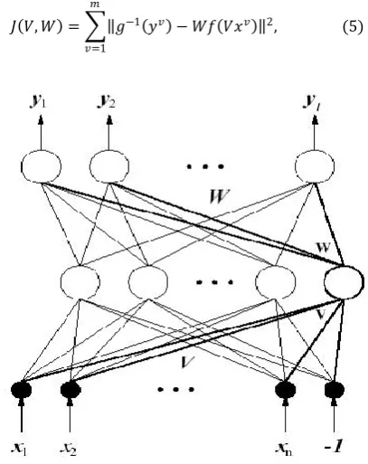
𝑡 , where 𝑉𝑗 = 𝑣𝑗1, 𝑣𝑗2, … , 𝑣𝑗 ,𝑛+1 𝑡and 𝑊𝑖= 𝑤𝑖1, 𝑤𝑖2, … , 𝑤𝑖 𝑡. This network is shown in fig 1 Let 𝑥𝑣, 𝑦𝑣 , 𝑣 = 1,2, … , 𝑚, be the training data for the network. We define an output error between the outputs of the network for the inputs 𝑥𝑣 and the relevant outputs 𝑦𝑣by
𝐽 𝑉, 𝑊 = 𝑔−1 𝑦𝑣 − 𝑊𝑓 𝑉𝑥𝑣 2, (5) 𝑚
[image:3.595.324.513.359.597.2]𝑣=1
Fig 1: Neural network before removing one unit in the hidden layer.
where𝑔−1 𝑦𝑣 = 𝑔−1 𝑦
1𝑣 , 𝑔−1 𝑦2𝑣 , … , 𝑔−1 𝑦𝑙𝑣 𝑡
is the inverse of the function, and . stands for the Euclidean norm. To determine 𝑉and 𝑊, we need to minimize the error function (5).
5.
CONVERGENCE RATE IN A
DESTRUCTIVE NEURAL NETWORK
WITHOUT THRESHOLDS IN THE
OUTPUT LAYER
In this section we will present the analysis of the convergence of the error in destructive neural network.
Let 𝑣 denote a connection weight vector between the ( + 1)-th hidden unit and 1)-the input layer, and let w be a weight vector connecting the ( + 1)-th hidden unit with the output layer. The ANN after removing the ( + 1)-th hidden unit is shown in Fig 2. We denote the weight matrices (𝑉, 𝑣) and (𝑊, 𝑤) by 𝑉 and 𝑊, respectively.
Then we can rewrite (5) as
𝐽 𝑉, 𝑊 = 𝑔−1 𝑦𝑣 − 𝑊 𝑓 𝑉𝑥𝑣 − 𝑤𝑓 𝑣. 𝑥𝑣 2 𝑚
𝑣=1 Where
𝑊𝑓 𝑉𝑥𝑣 = 𝑊 𝑓 𝑉𝑥𝑣 + 𝑤𝑓 𝑣. 𝑥𝑣 and𝑤 is the removing weight vector.
The function can be written as follows:
𝐽 𝑉, 𝑊 = 𝐽 𝑉 , 𝑊 − 2 𝑑 , 𝑤 + 𝑎 𝑤 2 6
Fig 2: Neural network after removing one unit in the hidden layer.
in which 𝑑and 𝑎denote
𝑑 = 𝑓 𝑣. 𝑥𝑣 𝑐𝑣 𝑚
𝑣=1 and
𝑎 = 𝑓2 𝑣. 𝑥𝑣 , 𝑚
𝑣=1
Where 𝑐𝑣= 𝑔−1 𝑦𝑣 − 𝑊𝑓(𝑉𝑥𝑣) and the symbol . , . indicates an inner product in 𝑅𝑙. When the vector 𝑣 is fixed, the vector 𝑤 which minimizes the error function by
𝑤 =𝑑
[image:3.595.66.270.459.716.2]So the error after removing a hidden unit can be expressed as 𝑐 𝑣 = 𝑔−1 𝑦𝑣 − 𝑊 𝑓 𝑉 𝑥𝑣
= 𝑔−1 𝑦𝑣 − 𝑊𝑓 𝑉𝑥𝑣 + 𝑤𝑓 𝑣𝑥𝑣 = 𝑐𝑣+𝑑
𝑎𝑓 𝑣. 𝑥𝑣 .
Furthermore, using the symbols𝐶 𝑖𝑡= (𝑐𝑖1, 𝑐𝑖2, … , 𝑐𝑖𝑚), 𝐶𝑖𝑡= 𝑐𝑖1, 𝑐𝑖2, … , 𝑐𝑖𝑚 and 𝑆𝑡 = 𝑆1, 𝑆2, … , 𝑆𝑚 with𝑠𝑣= 𝑓(𝑣. 𝑥𝑣), we have
𝐶 𝑖𝑡= 𝐶𝑖𝑡+ 1
𝑎𝐶𝑖𝑡𝑆𝑆𝑡. (7) Moreover we can rewrite (7) as
𝐶 𝑖𝑡= 𝐶𝑖𝑡 𝐼𝑚+1𝑎𝑆𝑆𝑡 = 𝐶𝑖𝑡𝛤1 𝑣 , where𝐼𝑚is the unit matrix and
𝛤1 𝑣 = 𝐼𝑚+ 𝑆𝑆𝑡
𝑎 . It is easy to show that the matrix 𝛤1 𝑣 satisfies
1 ≤ 𝛤1 𝑣 𝑈, 𝑈 𝑈 2 ≤ 2 for arbitrary vector 𝑈.
This shows that the error after determining the weight w between the hidden and output layers is not convergent. In addition, the eigenvalues of this matrix can be obtained as follows:
One propriety of the matrix 𝛤1 𝑣 is
𝛤1 𝑣 𝑈, 𝑈 = 𝑈 2+𝑎1 𝑆 , 𝑈 2
≤ 𝑈 2+1
𝑎 𝑆 2 𝑈 2= 2 (8) since 𝑎 = 𝑆 2, and the other is
𝛤1 𝑣 𝑈, 𝑈 = 𝑈 2+ 1
𝑎 𝑆 , 𝑈 2≥ 𝑈 2 (9) From (8) and (9) we get
1 ≤ 𝛤1 𝑣 𝑈, 𝑈 𝑈 2 ≤ 2
which implies
1 ≤ 𝑚𝑎𝑥 𝜆𝑣≤ 2
Where 𝜆𝑣, 𝑣 = 1, … , 𝑚 are the eigenvalues of the matrix 𝛤1 𝑣 .
Next, we calculate the eigenvalues of the matrix 𝛤1 𝑣 to examine the Convergence rate of the error in more detail. The matrix 𝛤1 𝑣 can be written as
𝛤1 𝑣 =
𝑧11 −𝑧12 … −𝑧1𝑚
−𝑧21 𝑧22 … −𝑧2𝑚
… … … …
−𝑧𝑚1 −𝑧𝑚2 … 𝑧𝑚𝑚
,
Where 𝑧𝑖𝑖= 1 + 𝑠𝑖2 𝑎, 𝑧𝑖𝑗 = −𝑠𝑖𝑠𝑗 𝑎, and 𝑧𝑖𝑗 = 𝑧𝑗𝑖. The characteristic equation of this matrix is
𝛾1 𝜆 =
𝜆 − 𝑧11 𝑧12 … 𝑧1𝑚
𝑧21 𝜆 − 𝑧22 … 𝑧2𝑚
… … … . … … … … … 𝑧𝑚1 𝑧𝑚2 … 𝜆 − 𝑧𝑚𝑚
= 0.
By putting 𝜂𝑖= (1 − 𝜆) 𝑎 𝑠𝑖2, we can reform γ1(𝜆)as follows:
γ1 𝜆 =− 𝑠𝑖 2 𝑚 𝑖=1
𝑎𝑚 𝐿1 𝜆 = 0, where
𝐿1 𝜆 =
𝜂1+ 1 1 … 1
1 𝜂2+ 1 … 1
… … … . . … … … . . … … 1 1 … 𝜂𝑚+ 1
.
The determinant 𝐿1 𝜆 can be transformed by Laplace theorem as
𝐿1 𝜆 = 𝜂𝑣+ 𝜂𝑣
𝑖−1
𝑣=1 𝑚
𝑖=1 𝑚
𝑣=1
𝜂𝑣
𝑚
𝑣=𝑖+1
= 𝜂𝑣
𝑚
𝑣=1
+ 𝜂𝑣
𝑚 𝑣=1
𝜂𝑖 𝑚
𝑖=1
.
Thus, we have
γ1 𝜆 =− 𝑠𝑖 2 𝑚 𝑖=1
𝑎𝑚 𝜂𝑣
𝑚
𝑣=1
+ 𝜂𝑣
𝑚 𝑣=1
𝜂𝑖 𝑚
𝑖=1
= 2 − 𝜆 1 − 𝜆 𝑚−1= 0. Hence the eigenvalues of this matrix are given by
𝜆 = 2, 1, … ,1,1.
This shows that the error after determining the weight w between the hidden and output layers is not convergent.
6.
CONVERGENCE RATE IN A
DESTRUCTIVE NEURAL NETWORK
WITH THRESHOLDS IN THE OUTPUT
LAYER
We consider the network with thresholds 𝜃𝑖, 𝑖 = 1, 2, … , 𝑙,in its output layer before removing one unit in the hidden layer. In this case, we can write
𝑦𝑖= 𝑔 𝑤𝑖𝑗
𝑗 =1
𝑓 𝑣𝑗𝑘𝑥𝑘 𝑛+1
𝑘=1
− 𝜃𝑖 , 𝑖 = 1, 2, … , 𝑙
whose simple form is
𝑦 = 𝑔 𝑊𝑓 𝑉𝑥 − 𝜃 ,where𝜃 = (𝜃1, 𝜃2, … , 𝜃𝑙) and𝑔 𝑊𝑓 𝑉𝑥 − 𝜃 = (𝑔 𝑊1. 𝑓 𝑉𝑥 − 𝜃1 , 𝑔 𝑊2. 𝑓 𝑉𝑥 − 𝜃2 , … , 𝑔 𝑊𝑙. 𝑓 𝑉𝑥 − 𝜃𝑙 ).
The error function that related to the present network takes the following form
𝐽 𝑉, 𝑊, 𝜃 = 𝑔−1 𝑦𝑣 − 𝑊𝑓 𝑉𝑥𝑣 + 𝜃 2. 𝑚
𝑣=1
We remove one unit from the hidden layer and represent removed weight vectors again by 𝑣and 𝑤. By removing one hidden unit, we can write the threshold vector θ as 𝜃 = 𝜃 + ∆𝜃.
The error function related to this network can be expressed as 𝐽 𝑉 , 𝑊 , 𝜃 = 𝑔−1 𝑦𝑣 − 𝑊 𝑓 𝑉 𝑥𝑣 + 𝜃 2,
𝑚
𝑣=1
where we have used again the symbols 𝑉 = (𝑉, 𝑣) and 𝑊 = (𝑊, 𝑤). The same procedure as in the previous section will be applied in order to determine 𝑤 and ∆𝜃 so that 𝐽 𝑉 , 𝑊 , 𝜃 is minimum. Since 𝑊𝑓 𝑉𝑥𝑣 = 𝑊 𝑓 𝑉𝑥𝑣 + 𝑤𝑓 𝑣. 𝑥𝑣 and 𝜃 = 𝜃 + ∆𝜃, we can decompose the error function 𝐽 𝑉 , 𝑊 , 𝜃 as
𝐽 𝑉 , 𝑊 , 𝜃 = 𝐽 𝑉, 𝑊, 𝜃 + 2 𝑓 𝑣. 𝑥𝜈 𝑞𝜈+ ∆𝜃, 𝑤 𝑚
𝜈=1
− 𝑓2(𝑣. 𝑚
𝜈=1
𝑥𝜈) 𝑤 2− 2 ∆𝜃 , 𝑞𝑣 − ∆𝜃 2, 𝑚
𝜈=1 𝑚
where
𝑞𝜈 = 𝑔−1 𝑦𝑣 − 𝑊𝑓 𝑉𝑥𝑣 + 𝜃.
By minimizing this error function, we can easily determine 𝑤 and ∆𝜃 as
𝑤 =𝑚𝑑1− 𝑎2𝑑2
𝑏 , (10) ∆𝜃 =𝑎2𝑑1− 𝑎1𝑑2
𝑏 , (11) where
𝑎1= 𝑓2 𝑣. 𝑥𝜈 𝑚
𝜈=1
,
𝑎2= 𝑓 𝑣. 𝑥𝜈 𝑚
𝜈=1
,
𝑑1= 𝑓 𝑣. 𝑥𝜈 𝑚
𝜈=1
𝑞𝜈,
𝑑2= 𝑞𝜈 𝑚
𝜈=1
,
𝑏 = 𝑚𝑎1− 𝑎22.
Now we consider the convergence rate of the error as in the previous section.
Since
𝑞𝜈= 𝑔−1 𝑦𝑣 − 𝑊 𝑓 𝑉 𝑥𝑣 + 𝜃
= 𝑔−1 𝑦𝑣 − 𝑊𝑓 𝑉𝑥𝑣 + 𝑤𝑓 𝑣. 𝑥𝑣 + 𝜃 − ∆𝜃 = 𝑞𝜈+ 𝑤𝑓 𝑣. 𝑥𝑣 − ∆𝜃,
we can write the error at i-th component in the output layer as 𝑞 𝑖𝜈= 𝑞𝑖𝜈+ 𝑤𝑖𝑓 𝑣. 𝑥𝑣 − ∆𝜃𝑖. (12)
From (10), the i-th component of w can be written as 𝑤𝑖=
𝑚 𝑏𝑑1𝑖−
𝑎2 𝑏 𝑑2𝑖
=𝑚 𝑏 𝑠𝜈𝑞𝑖𝜈
𝑚
𝜈=1
−𝑎2 𝑏 𝑞𝑖𝜈
𝑚
𝜈=1 =𝑚
𝑏 𝑡𝑄𝑖𝑆 − 𝑎2
𝑏 𝑡𝑄𝑖1 = 𝑄𝑡 𝑖
𝑚
𝑏𝑆 −
𝑎2 𝑏 1 . Similarly from (11), we can also write ∆𝜃𝑖as
∆𝜃𝑖= 𝑄𝑡 𝑖 𝑎𝑏2𝑆 −𝑎𝑏21 ,
Where 𝑡𝑄 𝑖= 𝑞 𝑖1, 𝑞 𝑖2, … , 𝑞 𝑖𝑚 , 𝑄𝑡 𝑖= 𝑞𝑖1, 𝑞𝑖2, … , 𝑞𝑖𝑚 , 𝑆𝑡 = 𝑠1, 𝑠2, … , 𝑠𝑚 , and 𝑡1= 1, 1, … , 1 with 𝑠𝜈=
𝑓 𝑣. 𝑥𝜈 .Hence, (12) can be rewritten as
𝑞 𝑖𝜈= 𝑞𝑖𝜈+ 𝑚
𝑏 𝑡𝑄𝑖𝑆𝑠𝜈− 𝑎2
𝑏 𝑡𝑄𝑖1𝑠𝜈− 𝑎2
𝑏 𝑡𝑄𝑖𝑆 + 𝑎1
𝑏 𝑡𝑄𝑖1 or,
𝑄 𝑖
𝑡 = 𝑄
𝑖 𝑡 𝐼
𝑚+ 𝑚
𝑏𝑆 𝑆𝑡 − 𝑎2
𝑏𝑆1 𝑆𝑡 − 𝑎2
𝑏 𝑡1+ 𝑎1
𝑏 1 1𝑡 = 𝑄𝑡 𝑖𝛤2 𝑣 ,
where
𝛤2 𝑣 = 𝐼𝑚+ 𝑚
𝑏𝑆 𝑆𝑡 − 𝑎2
𝑏 𝑆1 𝑆𝑡 − 𝑎2
𝑏 𝑡1+ 𝑎1
𝑏 1 1𝑡 . We will show that the matrix 𝛤2 𝑣 satisfies the stability condition
1 ≤ 𝛤2 𝑈 𝑣 𝑈, 𝑈 2 ≤ 2
for arbitrary vector 𝑈.
One propriety of the matrix 𝛤2 𝑣 is
𝛤2 𝑣 𝑈, 𝑈 = 𝑈 2+𝑚𝑏 𝑆, 𝑈 2−2𝑎𝑏2 𝑆, 𝑈 1, 𝑈
+𝑎1 𝑏 1, 𝑈 2
≤ 𝑈 2+𝑚
𝑏 𝑆 2 𝑈 2
≤ 2 𝑈 2. 13
and the other is
𝛤2 𝑣 𝑈, 𝑈 ≥ 𝑈 2+ 𝑚
𝑏 𝑆, 𝑈 − 𝑎2 𝑚 1, 𝑈
2
+1
𝑚 1 2 𝑈 2 =𝑚
𝑏 𝑆, 𝑈 − 𝑎2 𝑚 1, 𝑈
2
+𝑚
𝑏 𝑆 − 𝑎2 𝑚1, 𝑈
2
≥ 𝑚
𝑏 𝑆 −
𝑎2
𝑚1
2 𝑈 2
= 𝑈 2. (14)
From (13) and (14) we get
1 ≤ 𝑚𝑎𝑥 𝜆𝑣≤ 2,
Where 𝜆𝑣, 𝑣 = 1, … , 𝑚 are the eigenvalues of the matrix 𝛤2 𝑣 .
Next, we calculate the eigenvalues of the matrix 𝛤2 𝑣 to examine the Convergence rate of the error in more detail. The matrix 𝛤2 𝑣 can be written as
𝛤2 𝑣 =
𝑧11 𝑧12 … 𝑧1𝑚 𝑧21 𝑧22 … 𝑧2𝑚 … … … …
𝑧𝑚1 𝑧𝑚2 … 𝑧𝑚𝑚
,
Where𝑧𝑖𝑖= 1 +𝑚𝑠𝑖
2
𝑏 − 2𝑎2𝑠𝑖
𝑏 + 𝑎1
𝑏,𝑧𝑖𝑗 = 𝑚𝑠𝑖𝑠𝑗
𝑏 −
𝑎2 𝑠𝑖+𝑠𝑗
𝑏 +
𝑎1
𝑏, and 𝑧𝑖𝑗 = 𝑧𝑗𝑖.The characteristic equation of this matrix is
𝛾2 𝜆 =
𝜆 − 𝑧11 −𝑧12 … −𝑧12
−𝑧21 𝜆 − 𝑧11 … −𝑧2𝑚
…...………...
−𝑧𝑚1 −𝑧𝑚2 … 𝜆 − 𝑧𝑚𝑚
=
𝜆 − 1 + 𝑝11 𝑝12 … 𝑝1𝑚
𝑝21 𝜆 − 1 + 𝑝22 … 𝑝2𝑚
…...……….………...
𝑝𝑚1 𝑝𝑚2 … 𝜆 − 1 + 𝑝𝑚𝑚
Where
𝑝𝑖𝑖= −𝑚𝑢𝑖2 − 1 𝑚𝑏 , and𝑝𝑖𝑗 = − 𝑚𝑢𝑖𝑢𝑗 − 1 𝑚𝑏 , with 𝑢𝑖= 𝑠𝑖− 𝑎2 𝑚.By putting 𝑡𝑣= 𝑏(1 − 𝜆) 𝑚𝑢𝑣2 − 1, we can reform 𝛾2 𝜆 as follows:
𝛾2 𝜆 = 𝑢𝑖2 𝑚 𝑖=1
𝑚 𝑚
𝑏 𝑚−1
𝐿2 𝜆
=
𝜆 − 1 + 𝑝11 𝑝12 … 𝑝1𝑚 1
= 0,
𝑝21 𝜆 − 1 + 𝑝22 … 𝑝2𝑚 1
……….
𝑝𝑚1 𝑝𝑚2 … 𝜆 − 1 + 𝑝𝑚𝑚 1
with
𝐿2 𝜆 =
𝑡1 1 1 … 1 1
1 𝑢1
1 𝑡2 1 … 1 1 𝑢1
2 ………..
1 1 1 … 𝑡𝑚−1 1 𝑢1
𝑚 −1
1 1 1 … 1 𝑡𝑚
1 𝑢𝑚 1 𝑢1 1 𝑢2 1
𝑢3 …
1 𝑢𝑚 −1
1 𝑢𝑚
−𝑚2 𝑏 Using the Laplace theorem, we get
𝛾2 𝜆 = 𝑢𝑖2 𝑚 𝑖=1 𝑚 𝑚 𝑏 𝑚−1
−𝑚2
𝑏 𝐴 + 𝐵 , (15) where
𝐴 =
𝑡1 1 … 1
1 𝑡2 … 1
……….
1 1 … 𝑡𝑚
and
𝐵 = − 1
𝑢𝑖2𝑇𝑖+ 1 𝑢𝑖𝑢𝑗𝑇𝑖𝑗 𝑚 𝑗 =1 𝑗 ≠𝑖 𝑚 𝑖=1 𝑚 𝑖=1 with
𝑇𝑖=
𝑡1 1 … 0 … 1
, 1 𝑡2 … 0 … 1 ……..…………..
0 0 … 1 … 0
………
1 1 … 0 … 𝑡𝑚
Generally, we have
= (𝑡𝑣− 𝑎)
𝑚
𝑣=1
+ 𝑎 (𝑡𝑣− 𝑎)
𝑖−1
𝑣=1 𝑚
𝑖=1
𝑡𝑣− 𝑎 . 𝑚
𝑣=𝑖+1
According to the above result we can reform A,𝑇𝑖,and𝑇𝑖as follows:
𝐴 = (𝑡𝑣− 1)
𝑚
𝑣=1
+ (𝑡𝑣− 1)
𝑖−1
𝑣=1 𝑚
𝑖=1
𝑡𝑣− 1 , 𝑚
𝑣=𝑖+1
𝑇𝑖= (𝑡𝑣− 1)
𝑚 𝑣=1
(𝑡𝑖− 1) +
(𝑡𝑣− 1) 𝑚
𝑣=1
(𝑡𝑗− 1)(𝑡𝑖− 1) 𝑚
𝑗 =1 𝑗 ≠𝑖
,
and
𝑇𝑖𝑗 = (𝑡𝑣− 1)
𝑚 𝑣=1
(𝑡𝑖− 1)(𝑡𝑗− 1).
But we have 𝑡𝑣= 𝑏(1 − 𝜆) 𝑚𝑢𝑣2 − 1 and so it follows that
𝐴 = (2 − 𝜆) 1 − 𝜆 𝑚 −1 𝑏 𝑚
𝑚 1
𝑢𝑣2 𝑚
𝑣−1
(16)
and
𝐵 = − 1 𝑢𝑖2
𝑡𝑣− 1 𝑚
𝑣=1 𝑡𝑖− 1 𝑚
𝑖=1
− 1
𝑢𝑖2
𝑡𝑣− 1 𝑚
𝑣=1
𝑡𝑗 − 1 𝑡𝑖− 1 𝑚
𝑗 =1 𝑗 ≠𝑖 𝑚
𝑖=1
+ 1
𝑢𝑖𝑢𝑗
𝑡𝑣− 1 𝑚
𝑣=1
𝑡𝑗− 1 𝑡𝑖− 1 𝑚
𝑗 =1 𝑗 ≠1 𝑚
𝑖=1
= 1 𝑢𝑣2 𝑚
𝑣=1 (𝑏
𝑚 1 − 𝜆 )𝑚−2 −𝑚 1 − 𝜆
𝑏
𝑚− 𝑢𝑗2 𝑚
𝑗 =1 𝑗 ≠𝑖 𝑚
𝑖=1
+ 𝑢𝑖𝑢𝑗 𝑚
𝑗 =1 𝑗 ≠1 𝑚
𝑖=1
= 𝐾 − 1 − 𝜆 𝑏 − 𝑏 + 𝑏
𝑚−
𝑏 𝑚 = −𝑏𝐾(2 − 𝜆), (17) where
𝐾 = 𝑏
𝑚 1 − 𝜆
𝑚−2 1 𝑢𝑣2. 𝑚
𝑣=1
By substituting (16) and (17) into (15), we have
𝛾2 𝜆 = −𝐾(2 − 𝜆)2 𝑚𝑏 𝑚−21
𝑚 𝑢𝑖2= 0 𝑚
𝑖=1
which implies
(2 − 𝜆)2 1 − 𝜆 𝑚−2= 0,
and finally we obtain
𝜆 = 2, 2,1,1 … , 1.
This theorem shows that the error after determining the weight w and the correction ∆𝜃 between the hidden and output layers is not convergent.
Thus, we can conclude from the previous two sections that it is difficult to remove unit from the hidden layer after learning. On the other hand we can learn the neural networks by constructive learning, the description of this algorithm will be in the following section.
𝑇𝑖𝑗 =
𝑡1 1 … 0 … 1 … 1
1 𝑡2 … 0 … 1 … 1
………
0 0 … 1 … 0 … 0
………..
1 1 … 0 … 1 … 1
………
1 1 … 0 … 1 … 𝑡𝑚
𝑡1 a … a a
=
𝑡1−𝑎 0 … 0 a
a 𝑡2 … a a 𝑎
− 𝑡2 𝑡2
− 𝑎 … 0 a
……… ……
……… …………..
a a … 𝑡𝑚−1 a 0 0 … 𝑡− 𝑎 𝑚−1 a
a a a 𝑡𝑚 0 0 … 𝑎− 𝑡
7.
RULE EXTRACTION FROM
TRAINED NEURAL NETWORK USING
GENE EXPRESSION PROGRAMMING
A method to extract comprehensible rules from trained artificial neural network using gene expression algorithm will be described in this section.A constructive learning algorithm of three layered feedforward neural network [37,38,39] is described to train the network by supervised learning of the output layer and consequence conditions of the connections between the layers. Then GEP is carrying to obtain the rules which are bimodal with consistency. These consistencies can be described theoretically or observably. Consequently, the rule is the knowledge frame in system consistencies. Hence, the bimodal relation between rule and consistency is reversed in the form of relation between meaning and function. The technique described here uses GEP algorithms to generate rule patterns that progress into a set of suitable rules which clarify the reasons behind the classifications which neural networks make given different inputs. A Variety number of experiments by using different datasets will execute, and the obtained rules compared with those consequent from an illustrative package of data mining on the same datasets.
This technique is proposed to improve the unambiguousness of trained neural network that achieve classification tasks. It employ the trained neural networks to generate a set of instances their class label, and then extracts symbolic rules from those instances by GEP. Experiments with variety configurations show that, it can extract rules with high reliability that will describe the main function of trained neural network, or rules with powerful generalization ability that are even better than that are extracted from the trained neural network in prediction.
8.
EXPERIMENTAL RESULT
To evaluate our rule extraction algorithm, we used data sets such as:
8.1
Monk’s Task
In Monk's Task, an instance is characterized by six attributes 𝑎1, … . , 𝑎6 which have two, three, or four discrete possible values. Itmeans, for our learning algorithms we encoded the problems into a17 dimensional Boolean vector.
Monk #1: An example is mapped to a class "1" if and only if 𝑎1= 𝑎2 or (𝑎5= 1). In this problem, the training set contains 124 patterns for training and all 432 possible patterns are used to calculate the classification accuracy of the network.
The number of inputs of the network for Monk's problems is 17 binary inputs. Since the hidden units have a threshold, so we add another input represented by 1. Therefore the total inputs to the network under training are 18. We start the training of the network with one unit in the hidden layer. While the optimal weights of the network are obtained after adding another two hidden units. Hence the total number of the hidden units after training is 3.
The classification accuracy of the network is still the same as the original one.
The rules can be acquired by applying GEP to instances and the corresponding classes as classification problem. Before running GEP system, some parameters must be considered, the function set and terminal set for GEP are determined according to users knowledge for each problem. In this
experiment, the function set is the logical operators And, Or., Not, The terminal set consists of the attribute names, relational operators ( =, #), and attribute values of the data set being mined.
The obtained rules from running GEP are: Rule1: if A1 = 1 A2 = 1 then Class1 Rule2: if A5 = 1 then Class1
Rule3: if A1 = 3 A2 = 3 then Class1 Rule4: if A2 = 2 A1 = 2 then Class 1 default class #2
9.
RESULTS & DISCUSSION
To evaluate the performance of the learning algorithm we will use the commonly measures Accuracy, Precision, Sensitivity and Specificity [37]. The Accuracy is the number of correctly classified instances compared to the total number of instances presented to the system. It is defined as follows:
𝐴𝑐𝑐𝑢𝑟𝑎𝑐𝑐𝑦 = 𝑇𝑃 + 𝑇𝑁
𝑇𝑃 + 𝑇𝑁 + 𝐹𝑃 + 𝐹𝑁 (18)
Precision is the percentage of true positives compared to the total number of instances classified as positive events; one can define the precision as:
𝑃𝑟𝑒𝑐𝑖𝑠𝑖𝑜𝑛 = 𝑇𝑃
𝑇𝑃 + 𝐹𝑃 (19)
The sensitivity measure (also called recall rate) is the percentage of positive labeled instances that were predicted as positive. It is defined by:
𝑠𝑒𝑛𝑠𝑖𝑡𝑖𝑣𝑖𝑡𝑦 = 𝑇𝑃
𝑇𝑃 + 𝐹𝑁 (20)
The specificity is the percentage of negative labeled instances that were predicted as negative and it can be defined as:
specificity = 𝑇𝑁
𝑇𝑁 + 𝐹𝑃 (21)
where
TP (True Positives): is the number of instances covered by the rule which have the same class label as the rule.
FP (False Positives): is the number of instances covered by the rule which have a different class label from the rule.
FN (False Negatives): is the number of instances which are not covered by the rule but have the same class label as the rule.
TN (True Negatives): is the number of instances which are not covered by the rule and do not have the same class label as the rule.
software which consists of a collection of machine learning algorithms for data mining tasks such as REP Tree, Bayesian Networks, Radial Basis Function (RBF) Networks, and Single Conjunctive Rule Learner.
Table 1. The performance measures of various models for Monk 1.
Models Accuracy (%)
Precision (%)
Sensitivity (%)
Specificity (%) Nave
Bayesian 79.83 69.35 87.75 74.66
RBF
Network 83.06 77.41 87.27 79.71
REP
Tree 95.96 95.16 96.72 95.23
Bagging 100 100 100 100
Our
Model 100 100 100 100
The accuracy rate of the discovered rules was 100% for the problem, larger than the accuracy rate of the neural network and C4.5. In addition, neural networks via genetic algorithms have been used to extract rules [41] and the accuracy rate was 99.77% for monk1 problem. In the context of data mining this minor reduction in accuracy rate is a small price to pay for the large gain in the comprehensibility of the discovered knowledge.
10.
CONCLUSION
Research work in the area of extracting rules from trained neural networks has witnessed much activity recently. However, the knowledge obtained by ANNs is generally incomprehensible for humans.
In this paper we have introduced a method to extract accurate and comprehensible rules from a neural network and gene expression programming (GEP).
In the first part, we use ANNs that achieve high classification accuracy which was trained by constructive learning algorithm.
In the second part, an approach has been used for a gene expression algorithm to extract comprehensible rules from trained neural network for classification problems. From the features of instances and the labels of their classes we can use GEP to encode the rules in the form of logic expression. The system has been evaluated on some public domain data sets. The computational results have shown that the system extracted a very compact, comprehensible rule set without overly reducing the accuracy rate, in comparison with the accuracy rate of the rule set discovered by other methods. Widespread experiments have been carried out in this study to evaluate how well the proposed model performed on three benchmark classification problems in comparison with the other models. Finally, the results indicate that the proposed model is the superior compared with other model.
11.
REFERENCES
[1] Baesens, B., Setiono, R.; Mues, C., Vanthienen, J. 2003Using neural network rule extraction and decision tables for credit-risk evaluation. Manage. Sci., 49, 312-329.
[2] Jacobsson, H. 2005Rule extraction from recurrent neural networks: A taxonomy and review. Neural Comput.,17, 1223-1263.
[3] Kahramanli, H.; Allahverdi, N. 2009Rule extraction from trained adaptive neural networks using artificial immune systems. Expert Syst. Appl., 36, 1513-1522. [4] Setiono, R.; Baesens, B.; Mues, C. 2009A note on
knowledge discovery using neural networks and its application to credit screening, Eur. J. Operation. Res., 192, 326-332.
[5] Tickle, A.B., Andrews, R.; Golea, M.; Diederich, J. 1998The truth will come to light: Directions and challenges in extracting the knowledge embedded within trained artificial neural networks. IEEE Trans. Neural Netw.,9, 1057-1067.
[6] Setiono, R.; Leow, W.K. 2000FERNN: An algorithm for fast extraction of rules from neural networks.Appl. Intell.,12, 15-25.
[7] Baesens, B. T.,Gestel,V. S.,Viaene, M. Stepanova, J. Suykens and Vanthienen, J. 2003Benchmarking state of the art classification algorithms for credit scoring, vol. 56, no. 6, 627-635.
[8] Johansson, U., Konig, R. and Niklasson, L. 2005Automatically balancing accuracy and comprehensibility in predictive modeling.
[9] Thrun,S. e. a.,1991 The MONK's problems: A performance comparison of different learning algorithms, Pittsburgh, 91-197.
[10]Löfström,T. and Odqvist,P. 2004 RULE EXTRACTION IN DATA MINING - FROM A META LEARNING PERSPECTIVE.
[11]HumarK.,NovruzA., 2009"Rule extraction from trained adaptive neural networks using artificial immune systems", Expert Systems with Applications 36, 1513– 1522.
[12]LiMin. Fu, 1994 Rule generation from neural networks, IEEE Transactions on Systems, Man and Cybernetics, Vol. 24 No.8 , 1114-1124.
[13]Towell, G. and Shavlik,J. 1993TheExtraction of Refined Rules From Knowledge Based Neural Networks, Machine Learning, Vol. 131, 71-101. [14]Setiono, R.,Wee,K. H. and Zurada,M. J. 2002
Extraction of Rules from artificial neural network for nonlinear regression, IEEE Transaction Neural Networks, Vol. 23 No. 23, 564-577.
[15]Krishnan,R.,Sivakumar,G. and Bhattacharya,P. 1999 A search technique for rule extraction from trained neural networks, Pattern Recognit. Lett., vol. 20, no. 3, Mar., 273–280.
[17]Thrun,S. B. 1994Extracting provably correct rules from neural networks, in Technical Report IAI-TR-93-5, Institut fur Informatik III Universitat Bonn.
[18]Craven,M. W. 1996 Extracting comprehensible models from trained neural networks, Ph.D. Thesis, University of Wisconsin, Madison.
[19]OlcayB., 2002Extracting decision tree from trained neural networks, ACM SIGKDD International Conference on Knowledge Discovery and Data Mining, 456-461.
[20]Zhou, Z. H., Jiang, Y., Yang, Y. B. and Chen, S.F. 2003Extracting neural networks from trained neural network Ensembles, AI Communications, Vol. 16 No.1, 3-15.
[21]Garcez, A., d’Avila,S., Broda, K., Gabbay, D.M. 2001Symbolic knowledge extraction from trained neural networks: A sound approach, Artificial Intelligence, Vol. 125, 155-207.
[22]Tickle, A.B., Orlowski, M., and Diederich, J., 1996DEDEC: A Methodology for Extracting Rules from Trained Artificial Neural Networks, Proceedings of the Rule Extraction from Trained Artificial Neural Networks Workshop.
[23]Bojarczuk,C. C., Lopes, H. S., Freitas, A.A. and Michalk., 2004 A constrained-syntax genetic programming system for discovering classification rules: application to medial database. Artificial Intelligence in Medicine, Volume 30, Issue 1, 27-48. [24]Mitchell,M. MIT Press, 1996an Introduction to Genetic
Algorithms.
[25]Dudoit,S., Yang, Y. H., Callow, M. J. and Speed,T. P. 2002Statistical Methods for Identifying Differentially Expressed Genes in Replicated cDNA Microarray Experiments, StatisticaSinica, vol. 12, pages 111-139. [26]Reiner,A., Yekutieli, D. and Benjamini, Y.
2003Identifying ifferentially Expressed Genes Using False Discovery Rate Controlling Procedures, Bioinformatics, vol. 19, no. 3 , pages 368-375. [27]Efron,A.,Tibshirani,R.,Storey,J. D. and Tusher,V.
2001Empirical Bayes Analysis of a Microarray Experiment, J. Am. Statistical Assoc., vol. 96, pages 1151-1160.
[28]Creighton,C. and Hanash,S. 2003Mining Gene Expression Databases for Association rules, Bioinformatics, vol. 19, no. 1, 79-86.
[29]Brown, M. P. S. et al., 2000Knowledge-Based Analysis of Microarray Gene Expression Data by Using Support Vector Machines,Proc. Nat’l Academy of Sciences USA, vol. 97, no. 1, pages 262-267.
[30]Jiang, D., Tang,C. and Zhang, A. 2004Cluster Analysis for Gene Expression Data: A Survey, IEEE Trans. Knowledge and Data Eng., vol. 16, no. 11, (Nov.2004) pages 1370-1386.
[31]Pan,F. et al.,2003 “Carpenter: Finding Closed Patterns in Long Biological Datasets,” Proc. Ninth ACM SIGKDD Int’l Conf. Knowledge Discovery and Data Mining (KDD ’03).
[32]Cong ,G. et al., 2004Farmer: Finding Interesting Rule Groups in Microarray Datasets, Proc. ACM SIGMOD Int’l Conf. Management of Data (SIGMOD ’04). [33]Cong , G. et al., 2005Mining Top-k Covering Rule
Groups for Gene Expression Data, Proc. ACM SIGMOD Int’l Conf. Management of Data (SIGMOD ’05).
[34]Wang,H. C. and Lee,Y.S. 2005 Gene Network Prediction from Microarray Data by Association Rule and Dynamic Bayesian Network, Proc. Int’l Conf. Computational Science and Its Applications (ICCSA), pages 309-317.
[35]Shang,X. Q., Zhao, Q. and Li,Z. H. 2009Mining High-Correlation Association Rules for Inferring Gene Regulation Networks, Proc. 11th Int’l Conf. Data Warehousing and Knowledge Discovery (DaWaK ’09),pages 244-255.
[36]Pandey,G., Atluri, G.,Steinbach,M. and Kumar, V. 2008Association Analysis Techniques for Discovering Functional Modules from Microarray Data, Nature Precedings.
[37]Marghny. H. M, Minamoto,T. and Niijima,K. 1990”Rules extraction by constructive learning of neural networks and hidden unit clustering”, Lecture Notes in Artificial Intelligence, 1721, Springer, Proc. of the Second International Conference on Discovery Science, pages 343-344.
[38]Marghny. H. M, and Niijima,K. 2000”Extracting rules from neural network by removing unnecessary connections”, Proc. of the Second ICSC Symposium on Neural Computation, pages 322-328.
[39]Marghny. H. M, 2011 Rules extraction from constructively trained neural networks based on genetic algorithms
[40]WEKA at http://www.cs.waikato.ac.nz/~ml/wek. [41]Marghny. H. M, and Niijima,K., 2000 ” Redundant