Left Ventricle Statistical Models
Segmentation of Shape and Appearance for
Analysis of Cardiac MRI
Kayte Jaypalsing Natthusing
1Computer Science Dept. of CS &
IT, Dr. Babasaheb Ambedkar
Marathwada University,
Aurangabad(MH), India.
Sayyada Sara Banu
4,
Dept of CS and IT,
UniversityJizan University, Saudi
Arabia
Sumegh Shrikant Tharewal
2BSR Research Fellow, Dept. of CS
& IT, Dr. Babasaheb Ambedkar
Marathwada University,
Aurangabad(MH), India.
Kayte Sangramsing
5,
Dept of CS and IT,
CS & IT, Dr. Babasaheb Ambedkar
Marathwada University,
Aurangabad(MH), India.
Mohammed Waseem
Ashfaque
3Dept of CS and IT,
Dr. Babasheb Ambedkar
Marathwada University,
Aurangabad (MH) India,
Manza Ramesh Raybhan
6,
PhD
Assistant Professor of Computer
Science Dept. of CS & IT, Dr.
Babasaheb Ambedkar Marathwada
University, Aurangabad (MH), India.
ABSTRACT
This paper proposes a design of a framework structure for analysis of cardiac MRI to find out cardiovascular Disease easily and increase patent life. Segmentation of volumetric medical data is extremely time- consuming if using semi-automatically segmentation techniques with the first contribution involves the introduction of a new algorithm for fitting 4D Active Appearance Models on cardiac MRI, using the Simple interactive object extraction (SIOX), have observe a 43- fold increase in fitting accuracy that is on par with fuzzy clustering. We show the high quality results that are derived by the use of fuzzy clustering, and describe the ways in which it could improve the automated analysis of medical images.
Keywords:
MRI, SIOX, Fuzzy Clustering,1. INTRODUCTION
In 2010, Cardiovascular Disease (CVD) contributed to almost one third of global deaths. CVD is the leading cause of death in the developed world and by 2013; CVD is estimated to be the main cause of death in developing countries. According to 2001 estimates, if all forms of CVD in the India were eliminated, the average life expectancy would increase by around ten years. An elimination of all forms of cancer, on
Recently a lot of extensions for AAMs have been proposed. While the original AAMs work with gray value images in 2D, different strategies for adaptations to higher dimensions have been suggested. In theory such adaptations can be done straight forward. Practically there are some critical aspects. Different methods have been proposed to overcome the problems in higher dimensions. Applications include time-continuous (2D+time) segmentation of image sequences [Lelieveldt et al., 2001; Edwards et al., 1998], real-time combined 2D+3D AAMs [Xiao et al. 2004], and bi-temporal 3D AAMs [Stegmann and Pedersen, 2005]. Normally an increase in dimensionality inevitably causes a rapid increase of data. Especially the number of texture samples mounts significantly for higher dimensional data. Large data is the reason why methods for compression of texture data using wavelets [Wolstenholme and Taylor, 1999; Stegmann et al., 2004] or wedgelets [Darkner et al., 2004] recently have been proposed [2].
of this algorithm for the fitting of 3-D AAMs, when used for the segmentation of short axis cardiac MRI. By definition, short axis cardiac MR images are such that the long axis of the heart is perpendicular to the acquisition image plane. In practice, this means that during the AAM fitting we need to rotate our model only around the long axis of the heart. We take advantage of this fact to design an efficient fitting algorithm, which will rotate the model about the axis perpendicular to the image acquisition plane. To the best of our knowledge, this is the first effort at extending the inverse compositional image alignment algorithm to 3-D AAMs, and testing its applicability to the interpretation of medical images.
The algorithms described in the literature for fitting AAMs, can be classified as either robust but inefficient gradient descent type algorithms, or as the efficient but ad-hoc algorithms described next. The original AAM formulation uses regression to find a matrix R, such that if the current fitting error between the AAM and the image is δt, the updated AAM parameters are δp = Rδt. In more recent implementations, the estimation of matrix R is superseded by a faster and simpler method which regards R as a Jacobian matrix of the error function between the AAM and the image. In general, there is no reason why the error measure δt should uniquely identify the update parameters δp. Such methods lack a sound theoretical basis. Moreover, it has been shown that using a matrix R to estimate the update parameters can lead to suboptimal results. However, the constant matrix technique is widely used due to its fitting speed. Later, in, it was shown how to use the inverse compositional image alignment algorithm to fit 2-D AAMs.
The algorithm we describe in this paper is an extension of 3-D, under the constraint that all rotations take place around one axis. Our experimental results show that our algorithms border positioning errors are significantly smaller than the errors reported for other 3-D AAMs which use the constant matrix approach for the fitting. We perform experiments comparing our algorithm with Gauss-Newton based optimization, which is generally known as one of the most accurate and reliable optimization algorithms for such problems. We observe a 60-fold improvement in the fitting speed, with a segmentation accuracy that is as good - and in many cases better - as brute force Gauss-Newton optimization. We did not use any hierarchical coarse-to-fine methods during the optimization, to speed up the fitting process, however the effects of such an approach on the fitting algorithms could be a topic of future research
[image:2.595.317.545.68.354.2]This is an example of the basic Active Shape Model (ASM) and also the Active Appearance Model (AAM) as introduced by Cootes and Taylor, 2D and 3D with multi-resolution approach, color image support and improved edge finding method. Very useful for automatic segmentation and recognition of biomedical objects[2].
Figure 1. Hand Shape Appearance Model [4].
1.2 Functional Anatomy of Coronary
Vessels
Figure 2. An Anterior and posterior surfaces of the heart illustrating thelocation and distribution of the principal
coronary vessels13.
Coronary arterial blood passes through the capillary beds; most of it returns to the right atrium through the coronary sinus. Some of the coronary venous blood reaches the right atrium via the anterior coronary veins. In addition, vascular communications directly link the myocardial vessels with the cardiac chambers; these communications are the arteriosinusoidal, arterioluminal, and thebesian vessels. The arteriosinusoidal channels consist of small arteries or arterioles that lose their arterial structure as they penetrate the chamber walls, where they divide into irregular, endothelium-lined sinuses. These sinuses anastomose with other sinuses and with capillaries, and they communicate with the cardiac chambers. The arterioluminal vessels are small arteries or arterioles that open directly into the atria and ventricles. The the besian vessels are small veins that connect capillary beds directly with the cardiac chambers and also communicate with
automatically recognize if a contour is a possible/good object contour. Also the ASM modes contains matrices describing the texture of the lines perpendicular to the control point, these are used to correct the positions in the search step. After creating the ASM model, an initial contour is deformed by finding the best texture match for the control points. This is an iterative process, in which the movement of the control points is limited by what the ASM model recognizes from the training data as a "normal" object contour.
1.4 Basic idea AAM
PCA is used to find the mean shape and main variations of the training data to the mean shape. After finding the Shape Model, all training data objects are deformed to the main shape, and the pixels converted to vectors. Then PCA is used to find the mean appearance (intensities), and variances of the appearance in the training set. Both the Shape and Appearance Model are combined with PCA to one AAM-model.
By displacing the parameters in the training set with a know amount, and model can be created which gives the optimal parameter update for a certain difference in model-intensities and normal image intensities. This model is used in the search stage.
2. PROCESS OF DATA ANALYSIS IN
SIMPLE FORM
2.1 Image Analysis
Image analysis is the process of extracting meaningful information from images such as finding shapes, counting objects, identifying colors, or measuring object properties. Image Processing Toolbox provides a comprehensive suite of reference-standard algorithms and visualization functions for image analysis tasks such as statistical analysis, feature extraction, and property measurement.
2.2 Image Transforms
Image transforms play a critical role in many image processing tasks, including image enhancement, analysis, restoration, and compression. Image Processing Toolbox provides several image transforms, including Hough, Radon, FFT, DCT, and fan-beam projections. You can reconstruct images from parallel-beam and fan-beam projection data (common in tomography applications).
2.3 Hough Transform
The Hough transform is designed to identify lines and curves within an image. Using the Hough transform you can:
Find line segments and endpoints Measure angles
[image:3.595.333.528.607.721.2]2.4 Statistical functions
let you analyze the general characteristics of an image by: Computing the mean or standard deviation
Determining the intensity values along a line segment
[image:4.595.56.281.129.280.2] Displaying an image histogram Plotting a profile of intensity values
Figure 3.1 Identifying Round Objects Device-Independent Color Management
Device-independent color management enables you to accurately represent color independently from input and output devices. This is useful when analyzing the characteristics of a device, quantitatively measuring color accuracy, or developing algorithms for several different devices. With specialized functions in the toolbox, you can convert images between device-independent color spaces, such as sRGB, XYZ, xyY, L*a*b*, uvL, and L*ch.
Figure 3.2 Color-Based Segmentation Using the L*a*b* Color Space
3. METHODS
3.1 Optimization of 3D AAMs
for short axiscardiac MRI segmentation
Active appearance models (AAMs) provide a robust approach for the analysis of medical images (Cootes and Taylor, 1998, 2004). The ability of AAMs to learn the 3D structure of the heart and not lead to unlikely segmentations has stirred up interest in the medical imaging community regarding their use for the segmentation of the left ventricle from short axis cardiac MRI (Frangi et al., 2001; Mitchell et al., 2002).
Figure4 (A): Short axis cardiac MRI.
3.2. 3-D. Active appearance Model (AAMs)
In this section, we describe our implementation of the 3-D AAM of the left ventricle and its application for cardiac MRI segmentation. It has some similarities to the methodology used in but with many novel differences. We begin by quickly over-viewing point distribution models (PDMs) for 3-D AAMs. We proceed by describing how we align the landmarks which made up our training set and we conclude with an overview of how we handle appearance variation.Figure 4 (B): Endocardial and epicardial landmarks stacked on top of each other. displayed as curves for
greater clarity.
3.3 The Point Distribution Model
[image:4.595.317.540.341.455.2] [image:4.595.61.276.401.500.2]Assuming that we have a set of N sample shapes, each sample made up of l landmarks, we can represent each shape sample as a 3l dimensional vector, since each landmark is made up of 3 coordinates. Applying principal component analysis (PCA) on the distribution of the shape vectors, any shape s out of the N shapes can be represented as
For some p = (p1, ..., pn) ∈ _n, where s0 is the mean shape vector (a.k.a base mesh), and si indicates the ith eigenvector. We are summing over n eigenvectors si with eigenvalues λ1 ≥ λ2 ≥ ... ≥ λn ≥ 0. These are the n eigenvectors with highest eigenvalues that we found with PCA. We choose a value for n such that it accounts for around 90%-95% of the variation. Empirically, it has been hown that this is a good value. Higher values tend to lead to PDMs which overfit the training set, and much smaller values lead to PDMs which cannot generalize to new shapes. The greater the value of n, the better the approximation in becomes.
3.4 Appearance Variation
Here need to model the appearance variation of the volume enclosed by the shape. Firstly, we manually tetrahedrize s0, as shown in figure 4.C. This splits the left ventricular volume enclosed by s0 into tetrahedra whose appearance we model. In other words we are modeling the appearance of the interior of the LV (in the same way that Mitchell did in), and not just the appearance of the walls of the endocardium and epicardium. We use the same landmark connectivity defining the tetrahedra of s0 to define the tetrahedrization of any shape variation resulting from Equation above. Then, we sample the appearance enclosed by each training shape using the same methodology as in which is a 3D extension of the method described it for the 2D case: Firstly, we choose a set of sampling points inside each tetrahedron of s0. Each such point has a barycentric coordinate with respect to the tetrahedron enclosing it (by definition, the summation of the barycentric coordinates must equal 1). Then, we sample each tetrahedron in the training set at the same barycentric coordinates that we sampled its corresponding tetrahedron in s0. We review in more detail the definition of barycentric coordinates, and how to sample the interior of each tetrahedron.
Defines the different appearance variations the model has learned from our training data.
4. QUALITATIVE RESULTS
Above we have considered models which were matched to all data sets. In this section we concentrate on more details of individual AAM searches applied to selected single data sets. The intention is to show how different parameters influence the matching process.
4.1 Leave-One-Out
From the quantitative results it can be learned that data set number 13 leads to better matching results than data set number 18. The reason for this difference in quality of matches seems to be that data set 13 explains its appearance by modes that represent statistically frequent details. Data set 18 on the other hand seems to comprise statistically rare features.
Both data sets 13 and 18 were taken from the set of 15 data sets manually identified as qualitatively good. A leave-one-out test was carried leave-one-out such that for both data sets a model of the remaining 14 data sets was built and then matched with the one that was left out.
For both data sets multiple AAM searches were performed which differ in the initial displacements of the model’s position. Figure 5. shows the progress of matching in terms of APS. For all initial positions the model converges on data set 13. The matching of data set 18 proceeds not so stable and diverges for two of the four tests.
In the following we present results of matching the model from 14 good data sets to data set 13. Figure5.1. the model initially was displaced by 15mm in direction of the X- and by 30mm in direction of the Y-axis. Red color represents a point to- surface distance of 10mm or more. Blue indicates a point-to-surface distance of 5mm and green a distance of 0mm. Other color values are interpolated accordingly. The color coded surface distance is only calculated for individual model points and not over the whole surface. Colors are smoothly interpolated between points in the mesh. The black wire frame represents the shape of the ground truth for the considered data set 13.
Figure 5.1 shows the converged model together with the ground truth. Endoand epicardium of model and ground truth are shown separately.
[image:5.595.80.253.557.663.2]Figure 5: progress of show result area, Standard Deviation, or intensity of ENDO / EPI the cardiac MRI.
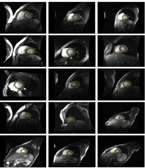
[image:6.595.324.554.75.396.2]Figure 5.1: Matching data set 13. The Result is shown for endocardium (left) and epicardium (right) separately[3].
Figure 5.2: Matching data set 13 (all iterations) with a model built from 14 data sets not including data set 13. The matching process starts at the image on the top left and ends at the right bottom. Each image represents one
iteration. [3]
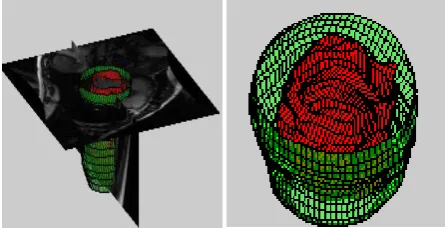
Figure 5.3: Matching data set 13 (difference volumes). This figure shows the initial difference volume, the difference volume after 4th, and after 8th (converged)
[image:6.595.317.572.485.621.2] [image:6.595.55.282.549.718.2]Figure 5.4: Matching data set 13 with slice-wise texture visualization. The top row shows three slices of data with the initial model superimposed. The second and third rows show the model after the 4th and 8th (converged) iteration respectively. The bottom row shows the data with the matched model’s shape points.
5. CONCLUSION
In this paper we have discussed 4D cardiac MRI data. We first presented an algorithm for fitting 4D active appearance models on short axis cardiac MR images, and observed an almost 43-fold improvement in the segmentation speed and a segmentation accuracy that is on par (and often better) with Simple interactive object extraction (SIOX), the most widely used algorithm for such optimization problems. We have outlined the importance of fast automatic and semiautomatic segmentation of such data. We shortly reviewed the anatomical background and outlined special properties of cardiac MRI data.
6. REFERENCES
[1] Medical Image Analysis 12 (2008) 335–357 Alexander Andreopoulos, John k. Tsotsos, York University , Dept of Computer science and Engineering, center for vision Research, Toronto, Ontario, Canada M3J 1P3
[2] American Heart Association, 2004. International Cardiovascular Disease Statistics. http://www.americanheart.org> (Online).
[3] 3D Active Appearance Models for Segmentation of Cardiac MRI Data durch Sebastian Zambal Matr. Nr.: 9826978 A - 3340 Waidhofen/Ybbs, Ybbsitzerstr. 44a. [4] Automatic Segmentation of Contrast Enhanced Cardiac
MRI for Myocardial Perfusion Analysis durch Andreas ch¨ollhuber Matr. Nr.: 0226055 A - 1040 Wien, Wiedner G¨urtel 24
[5] Manuel D. Cerqueira, Neil J.Weissman, Vasken Dilsizian, Alice K. Jacobs, Sanjiv Kaul, Warren K. Laskey, Dudley J. Pennell, John A. Rumberger, Thomas Ryan, and Mario S. Verani. Standardized myocardial segmentation and nomenclature for tomographic imaging of the heart. Circulation, 105(4):539–42, 2002.
[6] Baker, S., Matthews, I., 2001. Equivalence and efficiency of image alignment algorithms. In: Proceeding of the IEEE Conference on Computer Vision and Pattern Recognition, vol. 1, pp. 1090–1097.
[7] Baker, S., Goss, R., Matthews, I., 2004. Lucas-Kanade 20 years on: a unifying framework. Int. J. Comput. Vis. 56 (3), 221–255.
[8] Bardinet, E., Ayache, N., Cohen, L.D., 1996. Tracking and motion analysis of the left ventricle with deformable superquadrics. Med. Image Anal. 1 (2), 129–150. [9] Papademetris, X., Sinusas, A., Dione, D., Constable, R.,
Duncan, J., 2002.Estimation of 3D left ventricular deformation from medical imagesusing biomechanical models. IEEE Trans. Med. Imaging 21 (7), 786–800. [10]Davatzikos, C., Tao, X., Shen, D., 2003. Hierarchical
active shape models, using the wavelet transform. IEEE Trans. Med. Imaging 22 (3), 414–422.
[image:7.595.55.298.69.351.2]![Figure 1. Hand Shape Appearance Model [4].](https://thumb-us.123doks.com/thumbv2/123dok_us/8030999.768771/2.595.317.545.68.354/figure-hand-shape-appearance-model.webp)


![Figure 5.3: Matching data set 13 (difference volumes). This figure shows the initial difference volume, the difference volume after 4th, and after 8th (converged) iteration [3]](https://thumb-us.123doks.com/thumbv2/123dok_us/8030999.768771/6.595.324.554.75.396/figure-matching-difference-initial-difference-difference-converged-iteration.webp)