Munich Personal RePEc Archive
Estimating population means in
covariance stationary process
Halkos, George and Kevork, Ilias
University of Thessaly, Department of Economics
2006
Online at
https://mpra.ub.uni-muenchen.de/31843/
Estimating population means in
covariance stationary process
George Halkos and Ilias Kevork
Department of Economics, University of Thessaly
ABSTRACT
In simple random sampling, the basic assumption at the stage of estimating the standard error of the sample mean and constructing the corresponding confidence interval for the population mean is that the observations in the sample must be independent. In a number of cases, however, the validity of this assumption is under question, and as examples we mention the cases of generating dependent quantities in Jackknife estimation, or the evolution through time of a social quantitative indicator in longitudinal studies. For the case of covariance stationary processes, in this paper we explore the consequences of estimating the standard error of the sample mean using however the classical way based on the independence assumption. As criteria we use the degree of bias in estimating the standard error, and the actual confidence level attained by the confidence interval, that is, the actual probability the interval to contain the true mean. These two criteria are computed analytically under different sample sizes in the stationary ARMA(1,1) process, which can generate different forms of autocorrelation structure between observations at different lags.
Keywords: Jackknife estimation, ARMA, longitudinal data, actual confidence level
1. INTRODUCTION
The independence of observations in a sample of size n constitutes a vital condition for ensuring the validity of the produced confidence interval for the mean. Unfortunately, in a number of cases this condition does not hold. As representative examples we mention the set of generated estimates in Jackknife estimation, or the dynamic evolution of a social quantitative indicator in longitudinal studies. Additionally, we can mention the cases of constructing confidence intervals for the average delay of customers in service systems, or the determination of safety stock in continuous and periodic inventory systems. Accepting therefore a certain degree of dependency among observations at different lags, the application of the classical confidence interval estimator for the steady-state mean
2 1 2 2
1
2
n z X n
z
X o
n O
n
(1)
might lead to misleading results from the point of view of (a) the reliability of the standard error of the sample mean, and (b) the actual confidence level, that is, the actual probability the confidence interval to include the true population mean.
In the current paper, assuming that the data are generated from an ARMA(1,1) process, we investigate the consequences of using (1) for constructing confidence intervals. The choice of ARMA(1,1) is justified as, under different values of its parameters, alternative patterns of autocorrelation structure are observed. To study those consequences, two criteria have been used. The first refers to the ratio of the sampling error of (1) over the corresponding true sampling error which ensures equality among nominal and actual confidence levels. The second criterion concerns the differences between nominal and actual confidence levels, where the latter ones are computed analytically using (1) in samples from the ARMA(1,1). Unfortunately, the values of the previous two criteria are differentiated considerably between alternative form of autocorrelation structures, and on certain cases, the use of (1) in dependent series is prohibitive. Besides, the pattern of results in the current paper show a new direction of further research in a number of fields from social and business statistics.
2. LITERATURE REVIEW
realizations of stationary simulation output processes which guarantees both an adequate correspondence between actual and nominal confidence levels and a pre-specified absolute or relative precision, as these terms are defined by Law (1983). Law and Kelton (1982a) distinguish these methods as regenerative and non-regenerative. Fishman’s (1977) and Lavenberg and Sauer’s (1977) methods belong to regenerative category while the methods developed by Mechanic and McKay (1966), Law and Carson (1978), Adam (1983) and Heidelberger and Welch (1981a) have been characterized as non-regenerative.
For the truncation methods the objective is the elimination of initialization bias effects on the estimation of the steady-state mean. These methods provide estimators for the time point t* (1 t*n) for which the absolute value of the difference between the expected value
of the sample mean from the steady-state mean is greater than a pre-specified very small positive number e for any t<t*. Generating r replications of a simulation output process {X
t}
under the same initial conditions, some of the truncation methods estimate t* by applying the
truncation rule to each replication (Fishman 1971, 1973b; Schriber, 1974; Heidelberger and Welch, 1983). Some others, however, estimate t* from a pilot study, which is carried out on a
number of exploratory replications. Then the estimated value of t* is used as the global
truncation point in any other replication for which we use the same initial conditions (Conway, 1963; Gordon, 1969; Gafarian et al. 1978; Kelton and Law, 1983).
Fixed sample size confidence intervals methods propose different, asymptotically unbiased, estimators for the variance of the sample mean and these estimators may be used in the construction of confidence intervals. A number of confidence interval methods have been developed in the last decades in order to handle the problem.
The simplest fixed sample size confidence interval method is based on generating, for the process under consideration, k>1 independent replications of size m using independent steams of random numbers. When k is large enough, the variance of the k sample means is defined and used in the construction of confidence intervals, as these means are considered as independent, identical and normal random variables. But this method has practical difficulties, as it requires enormous systems and many hours of working time for the generation of just a single estimate.
Specifically, if {Xt} is a covariance stationary output process, the non-overlapping batch
means method is based on generating a single long replication of {Xt}. Then, this replication
is partitioned into k>1 contiguous and non-overlapping batches of size m. Provided that m is
large enough and
s s
, Law and Garson (1978) showed that the non-overlapping batch
means can be considered approximately uncorrelated and normal random variables. But as Song (1996) claims, the approximation of the correct batch size is possible but not trivial. At the same time, the construction of a confidence interval for a steady-state mean requires the satisfaction of normality and independency of the batch means.
Song and Schmeiser (1995) established the overlapping batch means method (OBM), which has smaller mean squared error in the estimation of the sample mean variance. Specifically, if n is the run length (sample size) of a single long replication of a covariance stationary output process {Xt}, the jth overlapping batch mean of size m [Xj(m)] may be
defined and in this context Welsh (1987) proposed for large m and n/m the following sample
mean variance estimator
n m 1
1 j
2 n j
2
OBM n(n mm 1) [X (m) X ]
ˆ . But Sargent et al. (1992)
claim that NOBM is preferable to OBM when we construct confidence intervals relying on small samples and probably equivalent in the case of using large samples.
Next, let us consider the standardized time series methods. If {Xt} is strictly stationary
(the joint distribution of Xt1, Xt2 ,...,Xtn is the same as the joint distribution of
s t s t s
t1 , X 2 ,...,X n
X for every t1, t2,…, tn and s) and assuming also that this process is phi-mixing (for large s the correlation of Xt and Xt+s becomes negligible; see Law, 1983), the
standardized time series methods use a functional central limit theorem to transform the sample X1, X2,…, Xn into a process which is asymptotically distributed as a Brownian Bridge
process. Dividing a single long replication into k>1 contiguous and non-overlapping batches of size m, for m large and by using Brownian Bridge properties, Schruben (1983) derived four methods for estimating the variance of the sample mean. The area method, the maximum method, the combined area non-overlapping batch means method and the combined maximum non-overlapping batch means method. The standardized time series methods are easy to use and asymptotically have advantages over NOBM, but require long runs.
In these lines and as a parametric time series modeling of simulation output data, we consider the autoregressive method of Fishman (1978). This method assumes that {Xt} is
Voss et al. (1996) derived good estimates of the steady state average queue delay using data from the transient phase of the simulation using a high-order AR(p) model. But such an autoregressive method is improper for widespread use as general ARIMA models are complex and assumptions for ARIMA modeling may be invalid for some particular simulation models.
The regenerative method was developed for the case in which the simulated process is characterized by the regenerative property and by enough regeneration cycles. This method was developed by Crane and Iglehart (1974a,b,c; 1975). Its principle is based on the identification of random points, where the process probabilistically starts over again. These points are called regeneration points. For instance, studying the delay in queue in the M/M/1 model, the indices of customers who find the system empty can be considered as regeneration points. The amount of data between two regeneration points is called the regeneration cycle. Then, the regeneration points are used to obtain independent random variables to which inferential methods can be applied. In this context, two methods have been developed for estimating the steady state mean and producing confidence intervals, the classical and the Jacknife. A very good description of these methods is provided in Law and Kelton (1982b). It is worth mentioning here that the main disadvantage of these methods is the identification of regeneration points, especially for complicated simulation models. Specifically, the problem with this method exists when either there are no regeneration points for the output process or when the simulation cannot produce enough cycles.
A new and more recent approach to simulation output analysis relies on resampling methods, such as the Jackknife and the Bootstrap (Quenouille, 1949; Tuckey, 1958; Efron, 1979; Efron and Tibshirani, 1993), which provide non-parametric estimates of bias and standard error. The Bootstrap method relies on pseudo-data created by re-sampling the actual data, but it requires independency, which is not always the case in simulation outputs. The application of this method to time series data may work by re-sampling sets of consecutive observations in order to capture the autocorrelation structure. Various forms of the Bootstrap method appear in the literature. First, the Moving Blocks Bootstrap (MBB), which relies on random re-sampling of fixed size overlapping blocks with replacement (Künsch, 1989; Liu and Singh, 1992; Hall et al., 1995). However, this method requires subjective inputs from the researcher and its estimates vary considerably.
Romano,1994). Under the same principle, Kim et al. (1993a) developed the Binary Bootstrap (BB) to analyze autocorrelated binary data. Kim et al. (1993b) introduced the Threshold Bootstrap (TB) extending the BB, and Park and Willemain (1999) modified the TB introducing the Threshold Jackknife (TJ). They claim that for various ARMA models, the TB has a better performance compared to MBB and SB in terms of estimating the standard error of the sample mean, if we optimize each sampling scheme with respect to the size of the re-sampling unit. They also show that the MBB has generally a poor performance.
Park et al. (2001) test the TB as a non-parametric method of output analysis and show that the TB is an effective alternative to the batch means and relatively easy. They also show that the TB is more effective in the construction of confidence intervals for the steady state mean and median delay in the M/M/1 model, and establish the asymptotic unbiasedness and consistency of the TB estimators when we refer to the sample mean.
Finally, we have the spectral method where the process {Xt} is assumed to be
covariance stationary. At zero frequency, the power spectrum f(0) is estimated either by using the Tukey spectral window (Fishman (1973 a,b; Duket and Pritsker, 1978; Law and Kelton, 1984) or by using the periodogram coordinates as presented in Heidelberger and Welch (1981a,b).
3. AUTOCCORELATION STRUCTURES IN ARMA(1,1)
ARMA(1,1) is defined by Xt Xt1t t1, where εt’s are uncorrelated and normal random variables with mean zero and common variance 2
. The model is stationary
when 1. Additionally, to overcome the invertibility problem regarding the MA component (the model produces the same ρ1 for θ and 1 ), the values of θ are restricted in
the interval (-1,1). Under the previous specifications, the autocorrelation function of ARMA(1,1) is given from s11
s , where
2 1 11 2
(2)
For any 1 and 1, the denominator of (2) is always positive. Thus the sign of ρ1
of autocorrelation function of the ARMA(1,1) is specified as follows in the following intervals of and θ:
Case 1: 0 1 and
In this case the autocorrelation function converges exponentially to zero with 0s 1, for any s0. Given , and increasing θ, the degree of autocorrelation between observations at different lags becomes greater. The same holds of we keep θ fixed and we increase .
Case 2: 0 1 and 1
In this case the autocorrelation function again converges exponentially to zero, but with 0
1
s , for any s0. Given and reducing θ, the autocorrelation structure becomes stronger. On the contrary, with θ fixed, the increase of leads in absolute value to smaller ρ1
but higher ρs’s for any s2
Case 3: 1 0 and
The autocorrelation function converges to zero oscillating between positive and negative values starting from a positive ρ1 (011). Keeping fixed and reducing θ, the
autocorrelation structure becomes stronger. On the contrary, for any θ, reducing , the autocorrelation coefficients are getting smaller and smaller in absolute terms only in low lags.
Case 4: 1 0 and
The autocorrelation function converges to zero again oscillating between positive and negative values but starting now from a negative ρ1 (110). Either keeping as fixed
and reducing θ, or keeping θ fixed and decreasing, we meet stronger autocorrelation structures.
Furthermore, when , the corresponding ARMA(1,1) generates independent random variables at different lags.
4. BIAS OF THE CLASSICAL ESTIMATOR FOR THE VARIANCE OF
THE SAMPLE MEAN
Given a sample of size n from a covariance stationary process, the variance of the sample mean is given by
o
sn n h
X
Var (3a)
1 1 1 2 1 n s ss ns
h (3b)
and ρs to be the sth lag theoretical autocorrelation coefficient between any two variables of the
process whose time distance is s. Any process
Xt,t1,2,3,...
is covariance stationary when its mean and variance do not change over time, as well as, the covariance between Xt and Xt+sdepends only on the lag s and not on their actual values at times t and t+s.
Replacing s s11 in (3b), the function h
s takes the following form for theARMA(1,1):
1 2
1 1 1 1 2 1 n
h s n
or
1 n,
1 2 1
h 1
s (4)
Where
1 n 1 , n n
Halkos & Kevork(2003) showed that for every 1,
n, always takes values in the interval (0,1). Incorporating this result into (4), the first two findings concerning the bias of the sampling error for the classical confidence interval estimator are:When the autocorrelation function converges exponentially to zero with 0s 1, or converges to zero oscillating between positive and negative values starting from a positive ρ1,
the use of the classical estimator for the variance of the sample mean underestimates the sampling error of the confidence intervals. This leads to actual confidence levels lower than the desired nominal ones.
On the contrary, when the autocorrelation function again converges exponentially to zero, but with 1s 0, or converges to zero again oscillating between positive and negative values but starting from a negative ρ1, the use of the classical estimator for the variance of the sample
5. ACTUAL CONFIDENCE LEVELS ATTAINED BY THE CLASSICAL
ESTIMATOR IN ARMA(1,1)
Given the random variables X1, X2, …, Xn from the ARMA(1,1) process, Halkos &
Kevork (2003) showed that the actual confidence level attained by the classical confidence interval estimator for the steady-state mean is given by:
*
2 *
2 *
2 1 2
Pr
1A zN Z zN zN
where
*
2N
z
is the cumulative distribution function of the standard normal evaluated at
12s 2 *
2
h z
z N
N
for a nominal confidence level 1N.
Tables 1, 2, 3, and 4 presents the actual confidence levels for each form of the autocorrelation function in ARMA(1,1) for 1N 0.95. The following important remarks are drawn:
(a) When the autocorrelation function converges to zero with all the autocorrelation coefficients to be positive, the actual confidence levels are lower than the nominal at every combination of , θ and n. The important element here is that as the sample size is getting larger and larger the discrepancies between the actual and the nominal confidence levels become greater. And unfortunately with heavy autocorrelation functions even with a sample of just twenty observations, the actual confidence levels drop even below of 0.50.
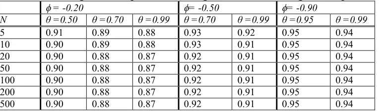
(b) With an autocorrelation function to converge to zero oscillating between positive and negative values with ρ1 to be positive, still the actual confidence levels are lower than the
nominal ones at every combination of , θ and n, but the discrepancies here are not large. Observe that with close to zero and θ close to 1, the differences between the actual and the nominal confidence level do not exceed 10%.
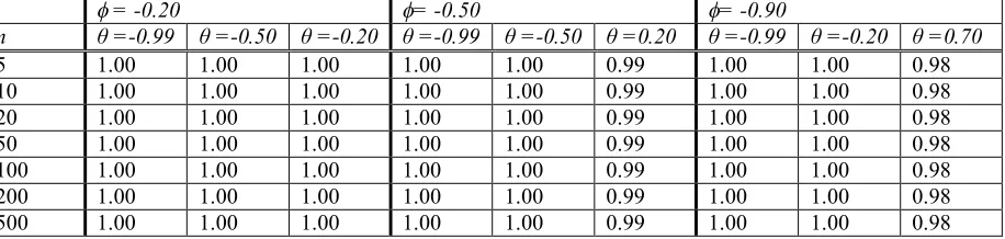
(c) On the contrary when the autocorrelation function converges to zero oscillating between positive and negative values but with ρ1 to be negative, the actual confidence levels are almost
(d) Finally, when the autocorrelation function converges to zero with all the autocorrelation coefficients to be negative, like the previous case, the actual confidence levels are higher than the nominal ones at every combination of , θ and n. As is approaching 0 and θ reaches1, we meet higher sampling errors than it should be, which for small samples are less than 10 times over the actual ones.
6. CONCLUSIONS
[image:11.595.63.535.443.558.2]The current paper illustrated that the performance of the classical confidence interval estimator for the steady-state mean in realisation from the ARMA(1,1) process depends upon the patterns of the autocorrelation structure. The first problematic case is met when the autocorrelation function converges exponentially to zero with all the autocorrelation coefficients to be positive. For such autocorrelation structures, although we believe that the reported point estimates are lying quite close to the actual values, in fact, due to the underestimation of the sampling error, the true mean might be quite far away from the reported estimate.
Table 1: Actual confidence levels when the autocorrelation function converges exponentially to zero with 0s 1
= 0.20 =0.50 =0.90
n θ =0.20 θ =0.50 θ =0.99 θ =0.20 θ =0.50 θ =0.99 θ =-0.20 θ =0.20 θ =0.99
5 0.87 0.83 0.82 0.78 0.76 0.76 0.67 0.65 0.65
10 0.85 0.82 0.80 0.74 0.72 0.71 0.54 0.53 0.52
20 0.85 0.81 0.79 0.72 0.70 0.69 0.46 0.44 0.43
50 0.84 0.80 0.79 0.71 0.69 0.68 0.39 0.38 0.37
100 0.84 0.80 0.79 0.71 0.69 0.68 0.37 0.36 0.35
200 0.84 0.80 0.79 0.71 0.68 0.67 0.37 0.35 0.35
500 0.84 0.80 0.79 0.71 0.68 0.67 0.36 0.35 0.34
Table 2: Actual confidence levels when the autocorrelation function converges exponentially to zero oscillating between positive and negative values starting from a positive ρ1
= -0.20 = -0.50 = -0.90
N θ =0.50 θ =0.70 θ =0.99 θ =0.70 θ =0.99 θ =0.95 θ =0.99
5 0.91 0.89 0.88 0.93 0.92 0.95 0.94
10 0.90 0.89 0.88 0.93 0.91 0.95 0.94
20 0.90 0.88 0.87 0.92 0.91 0.95 0.94
50 0.90 0.88 0.87 0.92 0.91 0.95 0.94
100 0.90 0.88 0.87 0.92 0.91 0.95 0.94
200 0.90 0.88 0.87 0.92 0.91 0.95 0.94
[image:11.595.71.453.624.737.2]Table 3: Actual confidence levels when the autocorrelation function converges to zero again oscillating between positive and negative values but starting from a negative ρ1
= -0.20 = -0.50 = -0.90
n θ =-0.99 θ =-0.50 θ =-0.20 θ =-0.99 θ =-0.50 θ =0.20 θ =-0.99 θ =-0.20 θ =0.70
5 1.00 1.00 1.00 1.00 1.00 0.99 1.00 1.00 0.98
10 1.00 1.00 1.00 1.00 1.00 0.99 1.00 1.00 0.98
20 1.00 1.00 1.00 1.00 1.00 0.99 1.00 1.00 0.98
50 1.00 1.00 1.00 1.00 1.00 0.99 1.00 1.00 0.98
100 1.00 1.00 1.00 1.00 1.00 0.99 1.00 1.00 0.98
200 1.00 1.00 1.00 1.00 1.00 0.99 1.00 1.00 0.98
500 1.00 1.00 1.00 1.00 1.00 0.99 1.00 1.00 0.98
Table 4: Actual confidence levels when the autocorrelation function converges exponentially to zero, but with 1s 0
= 0.20 =0.50 =0.90
n θ=-0.99 θ= -0.70 θ =-0.50 θ=-0.99 θ= -0.70 θ=-0.99
5 1.00 1.00 0.99 1.00 0.99 0.97
10 1.00 1.00 1.00 1.00 1.00 0.98
20 1.00 1.00 1.00 1.00 1.00 1.00
50 1.00 1.00 1.00 1.00 1.00 1.00
100 1.00 1.00 1.00 1.00 1.00 1.00
200 1.00 1.00 1.00 1.00 1.00 1.00
500 1.00 1.00 1.00 1.00 1.00 1.00
REFERENCES
Adam, N.R., 1983. Achieving a confidence interval for parameters estimated by simulation. Management Science, Vol.29, pp. 856-866.
Conway, R.W., 1963. Some tactical problems in digital simulation. Management Science, Vol. 10, pp. 47-61.
Crane, M.A., and D.L. Iglehart, 1974a. Simulating stable stochastic systems, I: General multi-server queues. Journal of the Association for Computing Machinery, Vol. 21, pp.103-113.
Crane, M.A., and D.L. Iglehart, 1974b. Simulating stable stochastic systems, II: Markov chains. Journal of the Association for Computing Machinery, Vol. 21, pp.114-123.
Crane, M.A., and D.L. Iglehart, 1974c Simulating stable stochastic systems, III: Regenerative processes and discrete event simulations. Operations Research, Vol. 23, pp.33-45.
Crane, M.A., and D.L. Iglehart, 1975. Simulating stable stochastic systems, IV: Approximation techniques. Management Science, Vol. 21, pp.1215-1224.
Ducket, S.D., and A.A.B. Pritsker, 1978. Examination of simulation output using spectral methods. Mathematical Computing Simulation, Vol. 20, pp. 53-60.
Efron, B., 1979. Bootstrap methods: Another look at the jackknife. The Annals of Statistics 7, 1-26
Efron, B. and Tibshirani, R., 1993. An Introduction to the Bootstrap. Chapman & Hall, New York.
Fishman, G.S., 1971. Estimating the sample size in computing simulation experiments. Management Science, Vol. 18, pp. 21-38.
Fishman, G.S., 1973a. Statistical analysis for queuing simulations. Management Science, Vol. 20, pp. 363-369.
Fishman, G.S., 1973b. Concepts and methods in discrete event digital simulation. John Wiley and Sons, New York.
Fishman, G.S., 1977. Achieving specific accuracy in simulation output analysis. Communication of the Association for computing Machinery, Vol. 20, pp. 310-315.
Fishman, G., 1978. Principles of Discrete Event Simulation. Wiley, New York.
Fishman, G., 1999. Monte Carlo: Concepts, Algorithms, and Applications. Springer, New York.
Gordon, G., 1969. System simulation. Prentice-Hall, Englewood Cliffs N.j.
Hall, P., Horowitz, J. and Jing, B.-Y., 1995. On blocking rules for the bootstrap with dependent data. Biometrika 82, 561-574.
Heidelberger, P., and P.D. Welch, 1981a. A spectral method for confidence interval generation and run length control in simulations. Communications of the Association for Computing Machinery, Vol. 24, pp. 233-245.
Heidelberger, P., and P.D. Welch, 1981b. Adaptive spectral methods for simulation output analysis. IBM Journal of Research and Development, Vol. 25, pp. 860-876.
Heidelberger, P., and P.D. Welch, 1983. Simulation run length control in the presence of an initial transient. Operations Research, Vol. 31, pp. 1109-1144.
Kevork, I.S, 1990. Confidence Interval Methods for Discrete Event Computer Simulation: Theoretical Properties and Practical Recommendations. Unpublished Ph.D. Thesis, University of London, London
Kim, Y., Haddock, J. and Willemain, T., 1993a. The binary bootstrap: Inference with autocorrelated binary data. Communications in Statistics: Simulation and Computation 22, 205-216.
Kim, Y., Willemain, T., Haddock, J. and Runger, G., 1993b. The threshold bootstrap: A new approach to simulation output analysis. In: Evans, G.W., Mollaghasemi, M., Russell, E.C., Biles, W.E. (Eds.), Proceedings: 1993 Winter Simulation Conference, pp. 498-502.
Kelton, D.W. and A.M. Law, 1983. A new approach for dealing with the startup problem in discrete event simulation. Naval Research Logistics Quarterly, Vol. 30, pp. 6410658.
Künsch, H., 1989. The jackknife and the bootstrap for general stationary observations. The Annals of Statistics 17, 1217-1241.
Lavenberg, S., S., and C. H. Sauer, 1977. Sequential stopping rules for the regenerative method of simulation. IBM Journal of Research and Development, Vol. 21, pp. 545-558.
Law, A.M., 1983. Statistical analysis of simulation output data. Operations Research, Vol. 31, pp. 983-1029.
Law, A.M., and J.S. Carson, 1978. A sequential procedure for determining the length of a steady state simulation. Operation Research, Vol. 27, pp. 1011-1025.
Law, A.M., and W.D. Kelton, 1982a. Confidence interval for steady state simulations: II. A survey of sequential procedures. Management Science, Vol. 28, pp. 560-562.
Law, A.M., and W.D. Kelton, 1982b. Simulation modelling and analysis. McGraw Hill, New York.
Law, A. and Kelton, W., 1991. Simulation Modeling and Analysis, second ed. McGraw-Hill, New York.
Liu, R. and Singh, K., 1992. Moving blocks jackknife and bootstrap capture weak dependence. In: Le Page, R., Billard, L., (Eds.), Exploring the Limits of Bootstrap. Wiley, New York, pp.225-248.
Mechanic, H., and W. McKay, 1966. Confidence intervals for averages of dependent data in simulation II. Technical report 17-202 IBM, Advanced Systems Development Division.
Park, D. and Willemain, T., 1999. The threshold bootstrap and threshold jackknife. Computational Statistics and Data Analysis 31, 187-202.
Park, D.S., Kim, Y.B., Shin, K.I. and Willemain, T.R., 2001. Simulation output Analysis using the threshold bootstrap, European Journal of Operational Research 134, 17-28.
Quenouille, M., 1949. Approximation tests of correlation in time series. Journal of Royal Statistical Society Series B 11, 68-84.
Schriber, T.J., 1974. Simulation using GPSS. John Wiley and Sons, New York.
Sargent, R.G., Kang, K. and Goldsman, D., 1992. An investigation of finite-sample behavior of confidence interval estimators. Operation Research 40, 898-913.
Schruben, L., 1983. Confidence interval estimation using standardized time series. Operations Research 31, 1090-1108.
Song, W.T., 1996. On the estimation of optimal batch sizes in the analysis of simulation output. European Journal of Operational Research 88, 304-319.
Song, W.T. and Schmeiser, B.W., 1995. Optimal mean-squared-error batch sizes. Management Science 41, 111-123.
Tukey, J., 1958. Bias and confidence interval in not quite large samples (Abstract). The Annals of Mathematical Statistics 29, 614.
Voss, P., Haddock, J. and Willemain, T., 1996. Estimating steady state mean from short transient simulations. In: Charnes, J.M., Morrice, D.M., Brunner, D.T.