On Return Periodof the Largest Historical Flood

(1)

http://dx.doi.org/10.4236/gep.2014.23019

On Return Periodof the Largest Historical

Flood

Witold G. Strupczewski

1

_{, Krzysztof Kochanek}

1

_{, Ewa Bogdanowicz}

2

1_{Institute of Geophysics, Polish Academy of Sciences, Księcia Janusza}_{, Warsaw, Poland} 2_{Institute of Meteorology and Water Management, Podleśna}_{, Warsaw, Poland}

Email: [email protected], [email protected], [email protected]

Received April 2014

Abstract

The use of nonsystematic flood data for statistical purposes depends on reliability of assessment both flood magnitudes and their return period. The earliest known extreme flood year is usually the beginning of the historical record. Even though the magnitudes of historic floods are properly assessed, a problem of their retun periods remains unsolved. Only largest flood (XM) is known during whole historical period and its occurrence carves the mark of the beginning of the historical period and defines its length (L). So, it is a common practice of using the earliest known flood year as the beginning of the record. It means that the L value selected is an empirical estimate of the lower bound on the effective historical length M. The estimation of the return period of XM based on its occurrence, i.e. _{M = L}ˆ _{, gives the severe upward bias. Problem is to}

estimate the time period (M) representative of the largest observed flood XM.From the discrete uniform distribution with support of the probability of the L position of XM one gets _{M = L}ˆ ₂

which has been taken as the return period of XM and as the effective historical record length. The efficiency of using the largest historical flood (XM) for large quantile estimation (i.e. one with return period T = 100 years) has been assessed using maximum likelihood (ML) method with various length of systematic record (N) and various estimates of historical period length _Mˆ _com-

paring accuracy with the case when only systematic records alone (N) are used. The i-th simula- tion procedure incorporates systematic record and one largest historic flood (XMi) in the period M which appeared in the Li year backward from the end of historical period. The simulation result for selected distributions, values of their parameters, different N and M values are presented in terms of bias (B) and root mean square error (RMSE) of the quantile of interest and widely discussed.

Keywords

Flood Frequency Analysis, Historical Information, Error Analysis, Maximum Likelihood, Monte Carlo Simulations

1. Introduction

(2)

flood quantile XT or design flood. The problems with the assessment stem from short time series (N = T),

un-known probability distribution function of annual peaks, error corrupted data, simplifying assumptions as of identical independently distributed (i.i.d.) data and, in particular, the stationarity of relatively long series. All these may cause a high uncertainty of upper quantile estimate. The only effect of a sample size is widely docu-mented for various distribution models and estimation methods. Inclusion into Flood Frequency Analysis (FFA) other sources of error would result in increasing uncertainty of design flood estimate. This is a feature not ap-preciated by the engineers as they desire to have only one value for designing flood related structures.

To improve the accuracy of estimates of upper quantiles all possible sources of additional information are used such as all independent peaks above the threshold, seasonal approach, regional analysis, record augment- tation by correlation with longer nearby records and augmentation of the systematic records by historical and paleoflood data.

Frequency analysis of flood data arising from systematic, historical, and paleoflood records has been pro-posed by several investigators (e.g. a review Stedinger & Baker, 1987, Frances et al., 1994). The use of non sys-tematic flood data for statistical purposes depends on reliability of assessment both flood magnitudes and their return period. If the historical record is available, you can find information about the floods larger than prevail-ing majority of floods reported in the systematic record and in particular about the largest of all reported floods. Serious difficulties are related to the availability and exhaustiveness of historical information, the quality and accuracy of historical sources. Depending on the parameter number and their method of estimation, the esti-mates of high quantiles are more or less sensitive to the largest observed floods.

The Gumbel, log Gumbel and Weibull distributions together with maximum likelihood method (ML) was considered by Frances et al. (1994). To assess the statistical profit from historical information the asymptotic variances of the quantile estimates got from the systematic records alone and the combined time–series were compared and in addition they were compared with computer simulation experiments’ results. The results of their study performed for define length (M) of historical period indicate that value of historical data for estimat-ing flood quantiles can be small or large dependestimat-ing on only three factors: the relative magnitudes of the length of the systematic record (N) and the length of the historical period (M); the return period (T) of the flood quan-tile of interest, and the probability threshold defining the historical floods.

Most often the first hydrological historical notice concerns a large flood and therefore it is not known what had happened before. Then the date of the first recorded historical flood determines (is taken as) the historical memory length L, i.e. L is the duration of nonsystematic period commencing on the large flood. Even if the magnitudes of historic floods are properly assessed, a problem of their retun periods remains unsolved. Many of the literature examples (specially Benson (1950), Dalrymple (1960), IACWD (1962), Zhang (1982) and NERC, (1975: p. 177)) deal with effective length of historical record M used for frequency analysis which is always a period from the first extraordinary flood to the beginning of the systematic record, i.e. L.

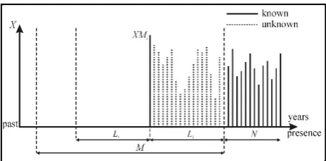
In other words, only the largest flood (XM) is known during whole historical period and its occurrence marks the beginning of the historical period and defines its length (L) (Figure 1). It is because the beginning of the historical period was somehow forced by the appearance of the largest flood then its magnitude (XM) likely cor-responds to a longer return period than L (or if in systematic record all observations are smaller than XM then to (L + N) - period). Consequently, the upward bias of the upper quantile estimates can be expected, if the histori-cal period of length L is taken in FFA as the nonsystematic observation period, or coming from an underestima-tion of the return period (Mˆ =L) of XM value.

Problem is to estimate the time period (M) representative of the largest observed flood XM, to evaluate the ef-ficiency of using the largest historical flood (XM) for large quantile estimation and to compare it with the case when only systematic records alone (N) are used. To keep and preserve for the FFA the unspoiled genuine in-formation contained in the observation (XM, L), the return period

( )

Mˆ of the largest observed historical flood XM should be assessed without using the data from the systematic record and only the information that the sys-tematic record does not contain the flood larger than the XM value is utilized. Every effort should be taken to establish M accurately on the basis of the occurrence of the largest recorded flood XM and an investigation of any information prior to XM event.

(3)

[image:3.595.198.427.83.196.2]

Figure 1. The case of N systematic and one largest flood in the beginning of historical period.

the year before the mentioned flood, it would also has been noted and commented (Hirsch & Stedinger, 1987). The same can be stated for horizon of two, three, four, etc. years. If we could identify this time span, we would have determined the upper limit of the empirical return period.

2. Literature Review

The earliest and simplest procedures for employing historical and paleoflood data were based on plotting posi-tions and graphical concepts (Zhang, 1982, 1985, Bernieur et al., 1986, Wang & Adams, 1984; Hirsch, 1985; Cohn, 1986). The common practice is using the earliest known flood year as the beginning of the historic record, i.e. taking Mˆ =L. The estimation of M based on the date of the first extraordinary flood occurrence exacer-bates the severe imprecision Defining as historical floods all floods during the M period above a given threshold and taking four different plotting position formulas, Hirsch and Stedinger (1987) have illustrated by Monte Carlo (MC) experiment the magnitude of the upward bias of the plotting position of the largest sample elements if the earliest known high flood year (L) is taken as the beginning of the historical record. Doing so they notice that L is a random variable, which is dependent on the flood-producing process itself that would be a violation of the assumption of the plotting position formulae.

Hosking and Wallis (1986b) use the MC computer simulation to assess whether a single paleoflood estimate, when included in a single-site ML flood frequency analysis procedures, it gives a worthwhile increase in the accuracy of estimates of extreme floods. They find that the main factors affecting the utility of this kind of pa-leological information are the specification of the fitted flood frequency (whether it has two or three unknown parameters) and the size of the measurement error of paleodischarge estimates. Errors in estimating the date of the paleoflood is considered as to be of minor importance. For distributions with higher CV or skewness the dif-ference between the effects of the errors of the magnitude of paleoflood and its return period is smaller.

Note that the randomness of the systematic records time series of i.i.d. variable can also be sometimes ques-tioned and undermined, for instance when the largest value XM of a time series intentionally terminates the N-elements’ systematic record. Then the XM is the last element of the N-element time-series. Such a case may arise when a water gauge was swept by a heavy flood (XM) and later not restored or intentionally as the conse-quence of the hydrological moving network design focused on the assessment of the variability range of annual peak flows. As before, the use of such a series in the FFA with Mˆ =L will lead to an overestimation of large quantiles.

3. Problem Formulation

The object of the paper is to assess by ML method whether there is any use for FFA of the largest flood termi-nating the time seriesassuming its magnitude (XM) is known. Therefore, the value of using the largest flood terminating observation period relative to using records without it is examined by comparing the bias (B) and the root mean square error (RMSE) of flood quantiles of two two-parameter distributions, namely Gumbel and Weibull while applying the simulation experiments. The emphasis is put on the effect of misspecification of the return period (M) of the largest historical (paleo-) flood (XM) and on the proper assesment of the M estimate on the basis of XM occurrence (L). So far the above case has not been presented in the hydrological literature.

(4)

gen-erally found to have desirable properties for combine systematic and historical information (Frances et al., 1994; Stedinger & Cohn, 1986; Naulet et al. 2005). It is assumed that the annual maximum floods are independent and identically distributed.

4. Assessment of the Return Period M of the XM flood

Dealing with the plotting positions Hirsch and Stedinger (1987) considered that the time of occurrence of the earliest documented historical flood L as the random variable defining a lower bound of the sample size used for computation of plotting positions. The position L of the largest in M period element (XM) (Figure 1) is the ran-dom variable being discretely uniformly distributed in the M period, i.e. pt = 1/M for t = 1, 2 … M. Obviously

the magnitude of the largest element (XM) is also a random variable. It can correspond in the population to a smaller or larger value of the exceedance probability than 1/M defining the true return period (MR) of the

ob-served XM, therefore, the difference (MR – L) is not restricted in sign.

Assume that the return interval (M) of XM is known. As L is unformly distributed variable in the M length time series with support L ∈ [0, 1, …, M], one gets E(L) = M/2 and V(L) = M2/12. In reality M is not known and its assesment is our goal. Taking the observed L value as the estimate of the expecting value, i.e. L = E(L) we get the M estimate equal Mˆ =2L. Because regardless of the estimation method the quantile estimators are not in

general linear function of Mˆ , the minimum bias of quantile

( )

ˆ = _ˆ

( )

ˆ − _

 

p p p

B x E x M x does not necessarily

correspond to the zero-bias of Mˆ , i.e. to Mˆ =2L. As in the systematic period (N) all its elements are smaller than XM, one can get Mˆ =2

(

L+N

)

.

5. Simulation Procedure

The simulation procedure described here incorporates N systematic record and one largest historic flood (XM) in the period M which appeared in the L year backward from the end of historical period (Figure 1). Obviously the systematic record and both magnitude (XM) and year of occurrence (L) randomly vary from simulation to simu-lation. As an estimate of the length of the historical period shall be successively Mˆ =L, 2L and the actual value Mˆ =M .

Generate a gauged record x1, x2, …, xN of independent random variates from the assumed (two-parameter)

flood-like distribution [F(x)] with parameters chosen to give specified values of CV.

Generate historical series of the same distribution of the length M, i.e. y1, y2, …, yM, and find the maximum

event (XM) of the historical series denoting the time (L) of its occurrence. Since the random variables (XM) and L are mutually independent the XM can be generated from the distribution of the largest element in a M-element series, i.e. F(M) = F1,M(y) = FM(y), while the corresponding time of its occurrence (L) from the discrete uniform

distribution with support {1, 2, …, M}.

Fit a flood frequency distribution by the method of maximum likelihood. If the fitted distribution has a distri-bution function F(x,θ) and a density function f(x, θ), where θ is a vector of unknown parameters, then the like-lihood function (L) is taken to be

(

)

ˆ 1

(

) (

)

(

)

1

; , − ; ; ;

=

 

= = ⋅ = _{⋅ } _



∏



L θ θ θ θ

N M

x x x i

i

x y F y XM f y XM f x , (1)

i.e., the use of incomplete data likelihood, where Mˆ =L, 2 and L M and for systematic record

( )

(

)

1

; ;

=

∏

L θ θ

N

x i

i

x f x . (2)

Calculate quantile estimates XˆT =F−1

(

1 1− T;θˆ

)

for Mˆ =L, 2 and L M and the systematic record (N)

only (i.e. when Mˆ =0), where F–1 is the inverse distribution function of the fitted flood frequency distribution, ˆ

θ is the maximum likelihood estimate of , and T is the return period of interest.

Repeat steps 1 – 4 a large number of times (i) and calculate the mean and variance of Xˆ_T, and hence the relative bias RB and relative RMSE of Xˆ_T taking Mˆi =Li, 2Liand M and the systematic record (N) only

(5)

(

)

1

1 1 ;

−

= −

T

X F T q

If in a generated series one gets max(x1, x2, …, xN) ≥ XM such a series is ignored which allows us to assume

ˆ ₌₂

M L.

6. Simulation Results

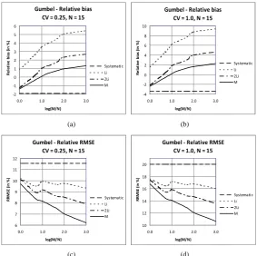
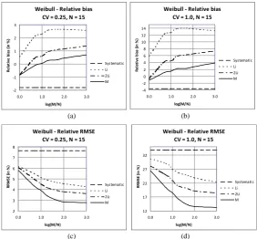
Results of simulation experiments are shown for Gumbel and Weibull distribution with four values of the coficient of variation CV = 0.25, 0.5, 0.75, 1.0, two length of systematic records N = 15, 50 and the length of ef-fevtive historical period M = Nexp(a) where a ∈ [0,3]. Due to the limited capacity of this paper without the loss of generality, only the selected results were presented in Figures 2-5, namely for CV = 0.25 and 1.0; the results for CV = 0.5 and 0.75 locate themselves between those presented in the Figures. Results got for the correct value of the return period (Mˆ =M ) are compared with those got for Mˆ =Li, 2Li. For completion the results for the

systematic record only (i.e. Mˆ =0) were presented in all Figures. Of course, for this case the results does not depend on M and, in consequence, on log(M/N).

7. Discussion Results

 The shorter the gauged record (N), the more useful historical information would be;

 Using as the estimate of the return period of largest historical flood (XM) the historical memory length (L) results in upward bias RB exceeding the bias got while using the systematic record only. Its value is growing with CV (and CS). It is accompanied by reduction of RMSE;

 Using in ML estimation the exact return period (M) of the largest historical flood (XM) the bias is reduced and RMSE is considerable lower;

(a) (b)

[image:5.595.171.455.374.656.2]

(c) (d)

Figure 2. Relative bias (RB) and relative root mean square error (RRMSE) of

100

ˆ

= T

X for gauge record length N = 15 as a function of historic period M for

ˆ ₌_0, _{, 2 ,} _.

i i i

M L L M Parent distribution Gumbel with CV equal: (a) 0.25 and (b)

1.0. Fitted distribution Gumbel.

Gumbel - Relative bias CV = 0.25, N = 15

-2 -1 0 1 2 3 4 5 6

0.0 1.0 2.0 3.0 log(M/N) Re la tiv e b ia s ( in % ) Systematic Li 2Li M

-4 -2 0 2 4 6 8 10

0.0 1.0 2.0 3.0 log(M/N) Re la tiv e b ia s ( in % ) Systematic Li 2Li M

Gumbel - Relative RMSE CV = 0.25, N = 15

6 7 8 9 10 11 12

0.0 1.0 2.0 3.0 log(M/N) RR M SE (i n % ) Systematic Li 2Li M

10 12 14 16 18 20

(6)

(a) (b)

(c) (d)

Figure 3. RB and RRMSE of XˆT=100 for gauge record length N = 50 as a

function of historic period M for Mˆi=0,Li, 2 ,L Mi . Parent distribution

Gumbel with CV equal (a) 0.25 and (b) 1.0. Fitted distribution Gumbel.

(a) (b)

(c) (d)

Figure 4. RB and RRMSE of XˆT=100 and gauge record length N = 15 for

historic period M for Mˆi=0,Li, 2 ,L Mi . Parent distribution Weibull with CV

equal (a) 0.25 and (b) 1.0. Fitted distribution Weibull.

-1.0 -0.5 0.0 0.5 1.0 1.5 2.0 2.5 3.0

0.0 1.0 2.0 3.0

log(M/N) Re la tiv e b ia s ( in % ) Systematic Li 2Li M

-1.0 0.0 1.0 2.0 3.0 4.0 5.0

0.0 1.0 2.0 3.0

4.0 4.5 5.0 5.5 6.0 6.5

0.0 1.0 2.0 3.0

log(M/N) RR M SE (i n % ) Systematic Li 2Li M

7.5 8.0 8.5 9.0 9.5 10.0 10.5 11.0

0.0 1.0 2.0 3.0

Weibull - Relative bias CV = 0.25, N = 15

-2 -1 0 1 2 3

0.0 1.0 2.0 3.0

-4 -2 0 2 4 6 8 10 12 14

0.0 1.0 2.0 3.0

Weibull - Relative RMSE CV = 0.25, N = 15

2 3 4 5 6 7 8

0.0 1.0 2.0 3.0

12 17 22 27 32

0.0 1.0 2.0 3.0

[image:6.595.172.455.80.354.2] [image:6.595.171.454.410.672.2]

(7)

(a) (b)

(c) (d)

Figure 5. RB and RRMSE of XˆT=100 and gauge record length N = 50 for

historic period M for Mˆi=0,Li, 2 ,L Mi . Parent distribution Weibull with CV

equal (a) 0.25 and (b) 1.0 and N = 50. Fitted distribution Weibull.

 Therefore to benefit from the largest historical observation every effort should be made to establish M accu-rately;

 In the absence of any information about the period preceding the occurrence of XM one should put Mˆ equal 2L or 2(L + N).

 The use of Mˆ =2L instead of Mˆ =L reduces the bias more than twice, but it is still ca 40% larger than the bias obtained at a known return period M of XM, and comparable or lower than the bias from systematic record (N) .

 The inclusion of the largest historical flood in FFA with Mˆ =2L (i.e. the effective historical record length) gives the substantial reduction in RRMSE of extreme flood estimates, however it is ca 40% lower than if the true M value would be available.

 The benefit from including the largest historical flood measured by the reduction of bias and RMSE depends on:

1) the length of systematic record (N),

2) the ratio of the true return period of XM, i.e. M to N, 3) the ratio of N to the return period of quantile of interest T, 4) the CV and skewness of the parent distribution.

8. Conclusions

Errors in historical data of course diminish the utility of the data for improvement the estimate of the flood mag-nitude at the given return period. In the simulations which produced Figures 2-5 it was assumed that the magni-tude of largest historical flood (XM) was measured without error and the same was assumed for systematic re-cord. It is realistic to suppose that the XM flood was measured much less accurate than the gauged rere-cord. Error in estimating the largest historical magnitude (XM) is much more important than error in estimating the date of its occurrence (e.g. Hosking & Wallis, 1986). It is significant that inspired by the practice of efforts to improve the accuracy of estimates of flood quantiles through a fuller use of the information they give just the opposite

-1.0 -0.5 0.0 0.5 1.0 1.5 2.0

0.0 1.0 2.0 3.0

-2 0 2 4 6 8

0.0 1.0 2.0 3.0

1.5 2.0 2.5 3.0 3.5 4.0 4.5

0.0 1.0 2.0 3.0

8 10 12 14 16 18

0.0 1.0 2.0 3.0

[image:7.595.172.455.83.349.2]

(8)

effect leading to increased uncertainty of flood estimates. On top of that, this already significant uncertainty is magnified by the unknown non-stationarity of the river’s regime over such a long time.

It remains to refer to the general problem of historical information when the applied distribution model is false, what is always the case (Strupczewski et al., 2002a, b; Węglarczyk et al., 2002). It is obvious that the dif-ferent distribution models fitted to the same systematic observations can give large differences in estimates of high quantiles. Supplementing systematic records by historical floods for FFA would reduce these differences and make the estimates more accurate. On the other hand, the uncertainty of the paleohistorical floods (both in terms of their magnitude and return period) combined with considerable increase of the complication of the problem (when compared to analysis of systematic data only) provoke a question whether the whole operation is worth a candle. Therefore, whether to include the palehistorical information or turn a blind eye to it is a matter of conscience.

Acknowledgements

This research project was partly financed by the grant of the Polish National Science Centre titled “Modern sta-tistical models for analysis of flood frequency and features of flood waves”, decision nr DEC-2012/05/B/ ST10/00482.

References

Benson, M. A. (1950). Use of Historical Data in Flood-Frequency Analysis. EOS Transaction on AGU, 31, 419-424. http://dx.doi.org/10.1029/TR031i003p00419

Bernieur, I., Miquel, J., Lebosse, A., & Griffet, A. (1986). Use of Additional Historical Information for Estimation and Goodness of Fit of Flood Frequency Model. Int. Symp. On Flood Frequency and Risk Analysis, L.S.U., Baton Rouge, 14-17 May 1986.

Cohn, T. A. (1986). Flood Frequency Analysis with Historical Information. Ph.D. Thesis, Cornell University.

Dalrymple, T. (1960). Flood Frequency Analysis. U.S. Geol. Surv. Water Supply Pap., 1543-A.

Frances, F., Salas, J. D., & Boes, D. C. (1994). Flood Frequency Analysis with Systematic and Historical or Paleoflood Data Based on the Two-Parameter General Extreme Value Models. Water Resources Research, 30, 1653-1664.

http://dx.doi.org/10.1029/94WR00154

Girguś, R., & Strupczewski, W. (1965). Excerpts from the Historical Sources Dealing with Extraordinary Hydro-Meteorolo- gical Phenomena on the Polish Territories from X-XVI c. Instr. i Podr., 87, 216 (in Polish).

Hirsch, R. M. (1985). Probability Plotting Positions for Flood Records with Historical Information. China Bilateral Sympo-sium on the Analysis of Extraordinary Flood Events, Nanjing, 21-23 October 1985.

http://dx.doi.org/10.1029/WR023i004p00715

Hirsch, R. M., & Stedinger, J. R. (1987). Plotting Positions for Historical Floods and Their Precision. Water Resources Re-search,23, 715-727. http://dx.doi.org/10.1029/WR022i004p00543

Hosking, J. R. M. and Wallis, J. R. (1986). Paleoflood Hydrology and Flood Frequency Analysis. Water Resources Research, 22, 543-550.

Interagency Advisory Committee on Water Data (IACWD) and U.S. Water Research Council Hydrology Committee (1982). Guidelines for Determining Flood Flow Frequency. Bull 17B, (Revised) Hydrol Subcomm, Office of Water Data Coord., U.S. Geol. Surv., Reston, Va.U.S. Gov. Print. Off. Washington D.C.

Natural Environment Research Council (NERC) (1975). Flood Studies Report. Vol. 1, London.

Naulet, R., Lang, M., Ouarda, T. B. M. J., Coeur, D., Bobee, B., Recking, A., & Moussay, D. (2005). Flood Frequency Analysis on the Ardèche River Using French Documentary Sources from the Last Two Centuries. Journal of Hydrology, 313, 58-78. http://dx.doi.org/10.1016/j.jhydrol.2005.02.011

Stedinger, J. R. and Cohn, T. A. (1986). Flood Frequency Analysis with Historical and Paleoflood Information. Water Re-sources Research,22, 785-793. http://dx.doi.org/10.1029/WR022i005p00785

Stedinger, J. R., & Baker, V. R. (1987). Surface Water Hydrology: Historical and Paleoflood Information. Review of Geo-physics, 25, 119-124. http://dx.doi.org/10.1029/RG025i002p00119

Strupczewski, W. G., Singh, V. P., & Weglarczyk, S. (2002a). Asymptotic Bias of Estimation Methods Caused by the As-sumption of False Probability Distribution. Journal of Hydrology,258, 122-148.

http://dx.doi.org/10.1016/S0022-1694(01)00563-7

(9)

Polonica,50, 279-319.

Wang, S. X., & Adams, B. J. (1984). Parameter Estimation in Flood Frequency Analysis. Publ. 84-02. Dep. Of Civ. Eng., Univ. of Toronto.

Węglarczyk, S., Strupczewski, W. G., & Singh, V. P. (2002). A Note on the Applicability of log-Gumbel and log-Logistic Probability Distributions in Hydrological Analyses: II. Hydrological Sciences Journal, 47, 123-137.

http://dx.doi.org/10.1080/02626660209492912

Zhang, Y. (1982). Plotting Positions of Annual Flood Extrems Considering Extraordinary Values. Water Resources Research, 18, 859-864. http://dx.doi.org/10.1029/WR018i004p00859