Two Phase Integrated Rule based Model (TPC-IRBM) for
Clustering of Gene Expression Data of CA1 Region of
Rat Hippocampus
Sudhakar Tripathi
Department of Computer Science& Engineering Indian Institute of Technology(BHU) Varanasi,India,221005
R.B.Mishra
Department of Computer Science & Engineering
Indian Institute of Technology(BHU) Varanasi,India,221005
ABSTRACT
This paper propose a semi supervised clustering model TPC-IRBM(Two phase clustering-Integrated rule based model) for clustering large data set such as gene expression data. TPC-IRBM works in two phases to cluster the gene expression data set. The proposed model is based on rule based models CRT,C5,CHAID and QUEST. In the first phase of the model 30 % data(which may vary) is extracted to prepare training, testing and validation data (TTV data)using suitable heuristic or neural network based clustering techniques. The output of first phase is used as build the models and generate the rule base fitting to TTV data using aforesaid models. The proposed model is then constructed by selecting and integrating the quality rules of various models using qualifying criteria corresponding to every cluster.The number of quality rules in proposed model is much more compared to that of CRT,C5,CHAID and QUEST.The performance in terms of accuracy is better compared to the models. Although in some cases Neural Network based models performance is slightly better but a very high cost of complexity for very large data set.
Keywords
Gene expression clustering,semi supervised clustering, integrated rule based model, two phase clustering,CA1 region gene expression clustering of rat hippocampus.
1.
INTRODUCTION
Clustering is very important technique in many data analysis applications. One of the most important applications is in bioinformatics. In bioinformatics clustering is mostly used to group genes whose expression patterns are available corresponding to various experimental(samples) or at various time points(time series). The most challenging task in clustering is to find actual number of clusters corresponding to given patterns of a dataset. Another is similarity measure; third one is how data is arranged. In bioinformatics clustering is very much useful because the genes that are co-expressed (belongs to same clusters) tend to have similar gene functions, premotor regulatory sequences and protein complexes. Clustering is the far most used method in gene expression analysis.
In some exceptional cases genes with nearly similar expressions may have different control strategies. After clustering a gene expression dataset into appropriate number of clusters we need not to evaluate individual gene functions, premotor sequences and protein complexes. Instead we can evaluate functions, premotor sequences and protein complexes of very few genes of various clusters and so genes
belonging to same cluster will have mostly same functions, premotor sequences and protein complexes. The main types of microarray data analysis include gene selection, clustering, and classification[19]. Piatetsky-Shapiro and Tamayo present one great challenge that data mining practitioners have to deal with. Microarray datasets -in contrast with other application domains- contain a small number of records (less than a hundred), while the number of fields (genes), is typically in thousands[20].
Large amount of gene expression data have been generated, but there is great requirement of developing the methods to analyze and explore the genes and related information [9].Clustering is much useful technique for the analysis of gene expression data. Many clustering algorithms are there which are being used to analyze gene expression data, including heuristic based like hierarchal[10],k-means[11], self organizing maps[12], graph theoretic approaches[13][14] and support vector machine[15] , Model based clustering[16],Bayesian model based clustering([17].
Many clustering techniques have been used to cluster gene expression dataset. But no one is reported to be widely efficient and acceptable in all cases due to various reasons. Because gene expression datasets are very large and expressed over very large samples or time series. It is more challenging to cluster gene expression datasets. So it is very difficult and time consuming to analyze genes corresponding to all experiments and time series expressions.
As not all the sample experiments and time expressions play role to corresponding cluster identification. We need such clustering techniques which can explore the expression regarding the importance of experiments (or time series). So that gene data sets can be clustered using only important feature expressions. Clustering in this way reduces overall effort and cost to cluster the genes for predictions of their functionalities.
Rest of the paper have been organized as follows: Section2: data sets, tools (implementation) Section3: methodology
Section4: cluster assessment Section 5: results and discussions
Section6: conclusions: summary, conclusion, future work, acknowledgement.
In our method we have used heuristic based algorithms(two-step, kohonens, k-means) for initial phase and on smaller data set. We have used the output of first phase to generate rule base which will be used to cluster rest of the data set originating from same or similar source.
As we have used rule based clustering technique for clustering the gene expression data sets. Rule based clustering techniques are easy to interpret and efficient. Once after second phase clustering model is generated it is simple and very fast to cluster the gene expression data sets with high efficiency and accuracy.
2.
DATA SET & IMPLEMENTATION
we have used subset of gene expression data of Rattus norvegicus (Rat) of hippocampal region for CA1 region of Gene expression profiling in differential cognitive outcomes in aging: CA1 from GEO database with geo_accession id GSE14723[18].
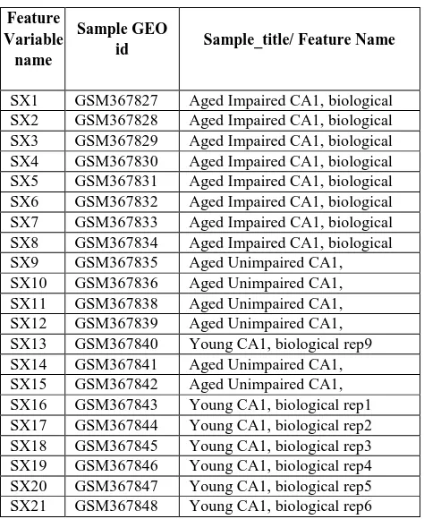
[image:2.595.53.290.470.760.2]The subset of CA1 expression data we used contains 3491 instances over 23 RNA samples from CA1 region of the hippocampi of young animals, aged animals with unimpaired spatial learning, and aged animals with impaired spatial learning. In the dataset there are 6 samples of aged (24-26 months old) male unimpaired (AU), 8 samples of aged (24-26 months old) male impaired (AI) and 9 samples of young (6 months old) male. Features, Sample GEO id and Feature names are shown in Table 1.
Table 1. Feature Variables of dataset. Feature
Variable name
Sample GEO
id Sample_title/ Feature Name
SX1 GSM367827 Aged Impaired CA1, biological rep1
SX2 GSM367828 Aged Impaired CA1, biological rep2
SX3 GSM367829 Aged Impaired CA1, biological rep3
SX4 GSM367830 Aged Impaired CA1, biological rep4
SX5 GSM367831 Aged Impaired CA1, biological rep5
SX6 GSM367832 Aged Impaired CA1, biological rep6
SX7 GSM367833 Aged Impaired CA1, biological rep7
SX8 GSM367834 Aged Impaired CA1, biological rep8
SX9 GSM367835 Aged Unimpaired CA1, biological rep1 SX10 GSM367836 Aged Unimpaired CA1,
biological rep2 SX11 GSM367838 Aged Unimpaired CA1,
biological rep4 SX12 GSM367839 Aged Unimpaired CA1,
biological rep5
SX13 GSM367840 Young CA1, biological rep9 SX14 GSM367841 Aged Unimpaired CA1,
biological rep7 SX15 GSM367842 Aged Unimpaired CA1,
biological rep8
SX16 GSM367843 Young CA1, biological rep1 SX17 GSM367844 Young CA1, biological rep2 SX18 GSM367845 Young CA1, biological rep3 SX19 GSM367846 Young CA1, biological rep4 SX20 GSM367847 Young CA1, biological rep5 SX21 GSM367848 Young CA1, biological rep6
SX22 GSM367849 Young CA1, biological rep7 SX23 GSM367850 Young CA1, biological rep8
We implemented all the methods
(CRT,C5,CHAID,QUEST)using SPSS Clementine 11.1 computing environment. Microsoft Excel have been used for all data storage and manipulation. C&RT(CRT) stands for Classification and Regression Trees, originally described in the book by the same name [1]. C5 (improvement of C4.5) is an algorithm used to generate a decision tree developed by Ross Quinlan[3][4][2].CHAID stands for Chi-squared Automatic Interaction Detector. It is a highly efficient statistical technique for segmentation, or tree growing, developed by Gordon V. Kass[5].QUEST stands for Quick, Unbiased, Efficient Statistical Tree. It is a relatively new binary tree-growing algorithm [6].
3.
METHODOLOGY
Two phase Clustering described in this research, works in two phases. In first phase actual number of clusters is predicted and then using any heuristic based algorithm which is efficient enough(we have used K-means) we can cluster the data set for training, testing,and validation. In second phase using training testing and validation data set we generate the models using CART,C5,Chaid & Quest techniques.After the models have been generated rule sets are generated corresponding to all models for clustering.Then we combine all the rule sets to generate a rule base. In rule base we select only those rules whose confidence factor are very high( greater than rcf). Then finally the clustering is performed using this rule based model. The rule based clustering is more efficient and of high quality compared to any of heuristic algorithm, decision tree or other rule based classifiers. The detailed description of the TPC-IRBM is as follows:
3.1 TPC Phase1: (See Figure1)
Step1: data preparation: 30% data have been selected from the original data set for predicting the actual no of cluster as well as preparing the training, testing and validation data set for phase2.
Step2: if actual number of clusters are known then this step is skipped else we have used two-step clustering(hierarchal) technique to find lower bound of number of clusters.Kohonens self-organizing map have been used to find upper bound of cluster number. Then we have used K-means(optionally any other efficient clustering method can be used) clustering technique for clustering the TTV data set from k= Clb to Cub.Here we have used proximity measure,
mean , standard deviation to predict actual number of clusters.as proximity measure of any pairs of clusters gets less than standard deviation, we stop and that is the predicted actual number of clusters.
On our data set applying this we got actual number of clusters predicted to be Kopt=6. Depending upon cases any one can
analyze the outcome with other measures and then predict the actual number of clusters.
Step3: After predicting actual number of clusters i.e. Kopt,
cluster the TTV data set using K-means for Kopt=6(optionally
Fig1.TPC-IRBM Phase1
3.2 TPC Phase2:
In phase 2(See Figure2) use T,T,V, data set outcome of phase1 to train, test and validate the the CRT,C5,Chaid,Quest models to generate the rule sets. From the rule sets generated from these models find out the importance factor of various features of patterns(experiments. Set threshold for importance factor that is acceptable to TI.Now use only those features(samples or experiments) whose Importance factor >= TI. Now find out those rules whose
confidence is greater than RCI(confidence threshold). Now
combine all the rules whose confidence >= RCI. Generated
from all models to produce a rule base to be used for clustering data set. Now this Rule bsed model will be validated with data set from GC1 to GC10. Then we will generalize the model for clustering.
Fig2.TPC-IRBM Phase2
Benefits of this approach are- Reduced experimentation required
(i) Improved rule base (ii) Data reduction
(iii) Improved efficiency in terms of speed and storage.
(iv) Although ANN models may give slightly better results but at much more cost of speed and storage. Experiment (samples) features are more to that compared with rule based model of TPC.
4.
RESULT & DISCUSSION
4.1 Phase 1 Result:
std.dev. . For our TTV dataset stopping criteria is met for K=6 which is the value of Kopt=6.Cluster proximities for k=2 to k=6 are shown in table2 and std dev. are shown in table3. For k=2 to k=6 cluster proximities are more or nearly equal than that of std.dev. but for k>6 it is overlapping or less than std. dev..So the Kopt=6 is taken as actual number of clusters.
Table 2. Cluster proximities for k=2 to k=6. Value
of K
Proximity of clusters
K= 2
C1 C2
C1 0 2.057
067 C2 2.057
067 0
K= 3
C1 C2 C3
C1 0 1.566
794 1.036
272 C2 1.566
794
0 2.602 987 C3 1.036
272 2.602 987 0 K= 4
C1 C2 C3 C4
C1 0 2.116
887 0.840
465 0.874
732 C2 2.116
887
0 2.957 285
1.242 218 C3 0.840
465 2.957
285
0 1.715 181 C4 0.874
732 1.242 218 1.715 181 0 K= 5
C1 C2 C3 C4 C5
C1 0 2.336
149 0.751 298 0.656 864 1.472 727 C2 2.336
149
0 3.087 398
1.679 351
0.863 525 C3 0.751
298 3.087
398
0 1.408 151
2.223 998 C4 0.656
864 1.679
351 1.408
151
0 0.815 892 C5 1.472
727 0.863 525 2.223 998 0.815 892 0 K= 6
C1 C2 C3 C4 C5 C6
C1 0 2.509
129 0.688 155 1.119 396 1.880 699 0.539 713 C2 2.509
129
0 3.197 239 1.389 823 0.628 499 1.969 497 C3 0.688
155 3.197
239
0 1.807 529
2.568 817
1.227 844 C4 1.119
396 1.389
823 1.807
529
0 0.761 376
0.579 716 C5 1.880
699 0.628 499 2.568 817 0.761 376
0 1.341 048 C6 0.539
[image:4.595.52.275.484.754.2]713 1.969 497 1.227 844 0.579 716 1.341 048 0
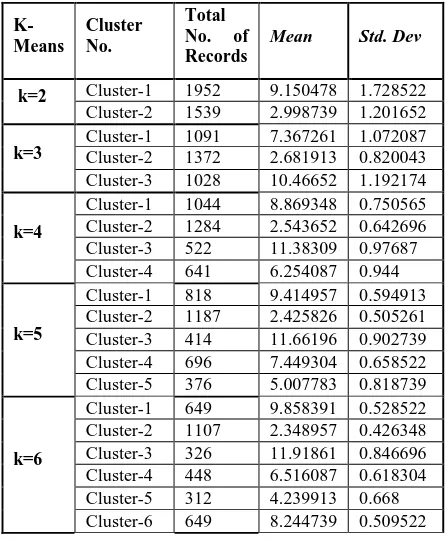
Table 3. Std deviation & means: for k=2 to k=6.
K-Means
Cluster No.
Total No. of Records
Mean Std. Dev
k=2 Cluster-1 1952 9.150478 1.728522
Cluster-2 1539 2.998739 1.201652
k=3 Cluster-1 Cluster-2 1091 1372 7.367261 2.681913 1.072087 0.820043
Cluster-3 1028 10.46652 1.192174
k=4
Cluster-1 1044 8.869348 0.750565 Cluster-2 1284 2.543652 0.642696 Cluster-3 522 11.38309 0.97687 Cluster-4 641 6.254087 0.944
k=5
Cluster-1
818 9.414957 0.594913 Cluster-2
1187 2.425826 0.505261 Cluster-3
414 11.66196 0.902739 Cluster-4
696 7.449304 0.658522 Cluster-5
376 5.007783 0.818739
k=6
Cluster-1
649 9.858391 0.528522 Cluster-2
1107 2.348957 0.426348 Cluster-3
326 11.91861 0.846696 Cluster-4
448 6.516087 0.618304 Cluster-5
312 4.239913 0.668 Cluster-6
649 8.244739 0.509522
After the estimation of Kopt=6 K-means algorithm is applied on TTV dataset and output cluster tags of instances are considered to be the classification tags for building predictive models of C%,CART,CHAID and QUEST. The output of K-means algorithm is output of phase1 that is dataset having 3491 instances tagged with cluster number. The number of instances ,mean and std.dev. are shown in table3.
4.2 Phase2 Result:
For phase two the TTV dataset is partitioned in three sets i.e. training dataset (2384 instances), testing dataset (758 instances) and validation dataset(349 instances).
The training data set is used to build the predictive models of C5,CART, CHAID and Quest. We have taken three metrics for analysis of the models i.e. features selected and their importance factor in model buiding, rules generated by the models with their confidence factor and predictive accuracy for training testing and validation datasets.
The features selected and their relative importance factor used in building each model are different. C5 model used 17 features, CART 10 features, CHAID 4 features and Quest 3 features out of total 23 features in training dataset. The most important feature in C5,CART, CHAID and QUEST are SX19,SX9,Sx9 and SX12 respectively and the least important are SX10,SX10,SX7,S15 respectively. Considering all models feature selection and relative importance only 17 features are selected at most out of which 7 features are having very less importance compared to others which can be ignored having negligible effect on results but we have taken all 17 features. Thus the large amount of data is reduced to considerable level which improves the efficiency in terms of time and space complexity as in bioinformatics a huge amount of data is available to analyze space and time complexity is major factor.
The rules generated by the models on training dataset are shown in table4 and their compositions are shown in table 5. The rules for each cluster generated by the models are shown along with number of instances and confidence factor of the rule. Higher confidence factor of the rule indicates lower misclassification and vice-versa. Total numbers of rules corresponding to all clusters generated by C5 are 32, by CART are 16, by CHAID are 11 and by QUEST are 7.Rule composition is done by logical OR operator.
Table4. Rule set generated by models after training C5 Rule Set Rule (R)
(No. of instances; Confidence factor)
Rules for Cluster 1
RC51
Rule 1 (5; 1.0) RC511
Rule 2 (9; 1.0) RC512
Rule 3 (4; 1.0) RC513
Rule 4 (407; 1.0) RC514
Rule 5 (5; 1.0) RC515
Rule 6 (5; 1.0) RC516
Rules for Cluster 2
RC52
Rule 1 (764; 1.0) RC521
Rule 2 (8; 1.0) RC522
Rule 3 (2; 1.0) RC523
Rules for Cluster 3 RC53
Rule 1 (3; 1.0) RC531
Rule 2 (208; 1.0) RC532
RC5
4 RC54 Rule 3 (279; 1.0) RC543
Rule 4 (3; 1.0) RC544
Rule 5 (6; 1.0) RC545
Rule 6 (8; 1.0) RC546
Rule 7 (2; 1.0) RC547
Rules for Cluster 5 RC55
Rule 1 (5; 1.0) RC551
Rule 2 (2; 1.0) RC552
Rule 3 (213; 1.0) RC553
Rule 4 (1; 1.0) RC554
Rule 5 (3; 1.0) RC555
Rules for Cluster 6 RC56
Rule 1 (2; 1.0) RC561
Rule 2 (1; 1.0) RC562
Rule 3 (6; 1.0) RC563
Rule 4 (3; 1.0) RC564
Rule 5 (5; 1.0) RC565
Rule 6 (398; 0.997) RC566
Rule 7 (18; 1.0) RC567
Rule 8 (1; 1.0) RC568
Rule 9 (3; 1.0) RC569
Default: Cluster
RC5df
2
Default
CRT Rule Set Rule
(No. of instances; Confidence factor)
RCR T
Rules for Cluster 1
RCRT1
Rule 1 (2; 1.0) RCRT11
Rule 2 (15; 0.6) RCRT12
Rule 3 (418; 0.995) RCRT13
Rule 4 (5; 1.0) RCRT14
Rules for Cluster 2 RCRT2
Rule 1 (771; 1.0) RCRT21
Rule 2 (2; 1.0) RCRT22
Rules for Cluster 3 RCRT3
Rule 1 (4; 0.75) RCRT31
Rule 2 (208; 1.0) RCRT32
Rules for Cluster 4 RCRT4
Rule 1 (295; 0.976) RCRT41
Rule 2 (6; 1.0) RCRT42
Rule 3 (4; 1.0) RCRT43
Rules for Cluster 5 RCRT5
Rule 1 (6; 0.833) RCRT51
Rule 2 (217; 0.991) RCRT52
Rules for Cluster 6 RCRT6
Rule 1 (9; 0.667) RCRT61
Rule 2 (414; 1.0) RCRT62
Rule 3 (8; 0.625) RCRT63
Default: Cluster 2 RCRTdf
CHAID Rule Set Rule
(No. of instances; Confidence factor)
RCH AID
Rules for Cluster
1 RCHAID1
Rule 1 (189; 0.746) RCHAID11
Rule 2 (26; 1.0) RCHAID12
Rule 3 (238; 1.0) RCHAID13
Rules for Cluster
2 RCHAID2
Rule 1 (715; 1.0) RCHAID21
Rules for Cluster
3 RCHAID3
Rule 1 (238; 0.887) RCHAID31
Rules for Cluster
4 RCHAID4
Rule 1 (239; 0.812) RCHAID41
Rule 2 (215; 0.507) RCHAID42
Rules for Cluster
5 RCHAID5
Rule 1 (238; 0.752) RCHAID51
Rules for Cluster
6 RCHAID6
Rule 1 (24; 1.0) RCHAID61
Rule 2 (238; 1.0) RCHAID62
Rule 3 (24; 0.833) RCHAID63
Default: Cluster
2 RCHAIDdf
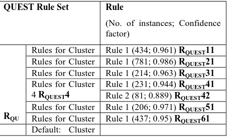
QUEST Rule Set Rule
(No. of instances; Confidence factor)
RQU EST
Rules for Cluster
1 RQUEST1
Rule 1 (434; 0.961) RQUEST11
Rules for Cluster
2 RQUEST2
Rule 1 (781; 0.986) RQUEST21
Rules for Cluster
3 RQUEST3
Rule 1 (214; 0.963) RQUEST31
Rules for Cluster
4 RQUEST4
Rule 1 (231; 0.944) RQUEST41
Rule 2 (81; 0.889) RQUEST42
Rules for Cluster
5 RQUEST5
Rule 1 (206; 0.971) RQUEST51
Rules for Cluster
6 RQUEST6
Rule 1 (437; 0.95) RQUEST61
Default: Cluster
[image:5.595.312.539.71.210.2]2 RQUESTdf
Table 5: Rule Composition For Each Cluster Corresponding To The Models Generating The Rules.
Number or Rules cluster wise
Total numbe r of rules C5 Rule Composition:
RC511 + RC512 +RC513 + RC514 + RC515
+ RC516 RC51
RC521+ RC522 + RC523 RC52
RC531 + RC532 RC53
RC541 + RC542 + RC543 + RC544 + RC545
+ RC546 +RC547 RC54
RC551 +RC552 + RC553 + RC554 + RC555 RC55
RC561 + RC562 + RC563 + RC564 + RC565
+ RC566 + RC567 + RC568 + RC569
RC56
Cluster1 (6 R) Cluster2 (3 R) Cluster3 (2 R) Cluster4 (7 R) Cluster5 (5 R) Cluster6 (9 R)
32 R
CRT Rule Composition:
RCRT11 + RCRT12 + RCRT13 + RCRT14
RCRT1
RCRT21 + RCRT22 RCRT2
RCRT31 + RCRT32 RCRT3
RCRT41 + RCRT42 + RCRT43 RCRT4
RCRT51 + RCRT52 RCRT5
RCRT61 + RCRT62 + RCRT63 RCRT6
Cluster1 (4 R) Cluster2 (2 R) Cluster3 (2 R) Cluster4 (3 R) Cluster5 (2 R) Cluster6 (3 R)
16 R
CHAID Rule Composition:
RCHAID11 + RCHAID12 + RCHAID13
RCHAID1
RCHAID21 RCHAID2
RCHAID31 RCHAID3
RCHAID41 + RCHAID42 RCHAID4
Cluster1 (3 R) Cluster2 (1 R) Cluster3 (1 R) Cluster4 (2 R) Cluster5
RCHAID51 RCHAID5
RCHAID61 + RCHAID62 + RCHAID63
RCHAID6
(1 R) Cluster6 (3 R)
QUEST Rule Composition:
RQUEST11 RQUEST1
RQUEST21 RQUEST2
RQUEST31 RQUEST3
RQUEST41 +RQUEST42 RQUEST4
RQUEST51 RQUEST5
RQUEST61 RQUEST6
Cluster1 (1 R) Cluster2 (1 R) Cluster3 (1 R) Cluster4 (2 R) Cluster5 (1 R) Cluster6 (1 R)
7 R
Coincidence matrices of all the models shows the accurately and misclassified number of instances for all clusters corresponding to rules generated by the model. The integrated rule based model is built by combining the qualifying rules generated by each model for each cluster. Qualifying rules are those rules whose misclassification is less than threshold set by the user in terms of percentage of total instances in actual cluster. Here we have set misclassification threshold to be 10 %. The qualifying rules are selected based on rule confidence factor and coincidence matrix applying the qualifying criteria.
[image:6.595.317.546.501.696.2]According to coincidence matrix of C5 all the rules are qualifying rules as misclassification is less than 10% for all rules. All rules of CART model are also qualifying rules as their misclassification is below 10%. For CHAID model rules generated for cluster 1 , cluster 4 and cluster 5 are misclassifying the instances more than acceptable limit hence for these clusters only the rules having confidence factor more than 0.8 are qualifying rules(threshold is optional for the user). For cluster 1 RCHAID12 and RCHAID13 have been selected as qualifying and RCHAID 11 as no qualifying rule, for cluster 4 RCHAID41 as qualifying rule and RCHAID42 as no qualifying rule and for cluster 5 there is only one rule RCHAID51 which is no qualifying. All rules of Quest model are also qualifying as their misclassification is less than 10%. Rules for integrated rule based model (TPC-IRBM) for each cluster are integration of all qualifying rules generated by each predictive model. The rule composition of integrated rule based model is shown in table6.
Table 6: Rule composition for each cluster corresponding to the TPC-IRBM model
Number or Rules cluster wise
Total number of rules
TPC-IRBM Rule Composition:
RC511 + RC512 +RC513 + RC514 + RC515
+ RC516+ RCRT11 + RCRT12 + RCRT13 +
RCRT14 + RCHAID12 + RCHAID13 +
RQUEST11 R1
RC521+ RC522 + RC523+ RCRT21 + RCRT22
+ RCHAID21+ RQUEST21 R2
RC531 + RC532+ RCRT31 + RCRT32 +
RCHAID31+ RQUEST31 R3
RC541 + RC542 + RC543 + RC544 + RC545 +
RC546 +RC547+ RCRT41 + RCRT42 + RCRT43
+ RCHAID41+ RQUEST41 +RQUEST42 R4
RC551 +RC552 + RC553 + RC554 + RC555+
RCRT51 + RCRT52 + RQUEST51 R5
RC561 + RC562 + RC563 + RC564 + RC565 +
RC566 + RC567 + RC568 + RC569 + RCRT61
+ RCRT62 + RCRT63 + RCHAID61 + RCHAID62
+ RCHAID63 + RQUEST61 RC56
Cluster1 (13 R) Cluster2 (7 R) Cluster3 (6 R) Cluster4 (13 R) Cluster5 (8 R) Cluster6 (16 R)
63 R
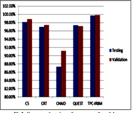
The accuracy of each predictive model for training, testing and validation dataset is compared. The accuracy of C5 model is highest i.e. 99.96% for training dataset, 98.15 % for testing dataset and 98.85 % for validation dataset. For CART it is 98.95% for training dataset, 96.97% for testing dataset and 97.42% for validation dataset. For QUEST it is 96.39% for training dataset, 97.36 % for testing dataset and 97.13% for validation dataset. For CHAID it is lowest and is 87.88% for training dataset, 87.34 % for testing dataset and 91.12% for validation dataset.
Fig3. Comparative view of accuracy of models
5.
CONCLUSION
Proposed method in this article is quite useful and easy to implement for clustering large biological data with large number of features. Rules generated by integrating the qualifying rules of various rule based model are high quality rules to achieve higher accuracy with much less complexity compared to neural network clustering methods,graph based and model based clustering methods with very marginal improvement in predicted accuracy for semi supervised clustering.
6.
FUTURE WORK
As the proposed model works in two phases. First phase for generating and preparing TTV data for second phase. We have used K-means clustering method in first phase and Heirarichal ,SOM for estimation of lower and upper number of clusters respectively. More robust methodology can be applied to improve the quality of prediction and clustering in first phase.In second phase the criteria that we have chosen for qualifying rules to be used in TPC-IRBMis confidence factor(misclassification rate) as threshold. The other criteria for rule integration and qualification can be explored in future work.
7.
REFERENCES
[1] Breiman, L., J. H. Friedman, R. A. Olshen, and C. J. Stone. 1984. Classification and Regression Trees. New York: Chapman & Hall/CRC.
[2] Quinlan, J. R. C4.5: Programs for Machine Learning. Morgan Kaufmann Publishers, 1993.
[3] Quinlan, J. (1996). Bagging, Boosting, and C4.5, Proceedings of the Thirteenth National Conferenceon Artificial Intelligence, Portland , Oregon (American Association for Artificial Intelligence Press, Menlo Park, California), pp. 725 – 730.
[4] Rulequest Research. (2013) See5/c5.0.[Online]. Available: http://www.rulequest.com/see5-info.html. [5] Kass, Gordon V.; An Exploratory Technique for
Investigating Large Quantities of Categorical Data, Applied Statistics, Vol. 29, No. 2 (1980), pp. 119–127. [6] Loh, W. Y., and Y. S. Shih. 1997. Split selection
methods for classification trees. Statistica [7] www.ncbi.nlm.nih.gov
[8] Clementine® 11.1 Algorithms Guide , Copyright © 2007 by Integral Solutions Limited.
[9] Lander E.S. , “Array of hope,” Nature genet.,21,3-4,1999.
[10] Eisen,M.B. et al., “ Cluster analysis and display of genome-wide expression patterns,” Proc. Natl. Acad. Sci. Am., 95, 14863–14868, 1998..
[11] Tavazoie,S. et al., “ Systematic determination of genetic network architecture,” Nat. Genet., 22, 281–285, 1999.. [12] Tamayo P. et al., “Interpreting patterns of gene
Expression with self organizing maps: methods and application to hematopoieitic differentiation,” Proc. Natl acad.Sci. USA,96,2907-2912,1999.
[13] Ben-Dor,A. and Yakhini Z., “clustering gene Expression patterns,” inRECOMB99: Proceedings of the third annual international conference on computational molecular biology. Lyon,france,1999,pp.33-42.
[14] Hartuv E. et al., “An algorithm for clustering cDNAs for gene expression analysis,” in RECOMB99: Proceedings of the third annual international conference on computational molecular biology. Lyon,france,1999, pp.188-197.
[15] Browm M.P.S., et al., “Knowledge based analysis of micro array gene expression data using support vector machine,” Proc. Natl acad.Sci. USA,97,262-267, 2000. [16] Yeung K.Y.,et al., “Model based clustering and data
transformations for gene expression data,” Bioinformatics , Vol. 17 no. 10 2001, 2001, pp.977-987. [17] Moyses Nascimento, et al., “ Bayesian model based
clustering of temporal gene expression using autoregressive panel data approach,” Bioinformatics,Vol. 28 no. 15 2012, 2012, pp. 2004-2007.
[18] Haberman RP, Colantuoni C, Stocker AM, Schmidt AC et al. Prominent hippocampal CA3 gene expression profile in neurocognitive aging. Neurobiol Aging 2011 Sep;32(9):1678-92. PMID: 19913943
[19] C G. Piatetsky-Shapiro, T. Khabaza, S. Ramaswamy apturing Best Practice for Microarray Gene Expression Data Analysis, , in Proceedings of KDD-2003 (ACM Conference on Knowledge Discovery and Data Mining), Washington, D.C., 2003.