Munich Personal RePEc Archive
Can Information Asymmetry Cause
Agglomeration?
Berliant, Marcus and Kung, Fan-chin
31 October 2006
Can Information Asymmetry Cause
Agglomeration?
Marcus Berliant
Department of Economics, Washington Universityy
and
Department of Economics and Finance, City University of Hong Kong
Fan-chin Kung
Department of Economics and Finance, City University of Hong Kongz
and
Institute of Economics, Academia Sinica, Taiwan
April 2007
Abstract
The modern literature on city formation and development, for exam-ple the New Economic Geography literature, has studied the agglomeration of agents in size or mass. We investigate agglomeration in sorting or by type of worker, that implies agglomeration in size when worker populations di¤er by type. This kind of agglomeration can be driven by asymmet-ric information in the labor market, speci…cally when …rms do not know
The authors are very grateful to the Department of Economics and Finance at City Univer-sity of Hong Kong for funding that facilitated their collaboration. We thank Sukkoo Kim for help with data, and Guido Cataife, Tom Holmes, Bob Hunt, Tomoya Mori, Gianmarco Otta-viano, Will Strange, Matt Turner, and Ping Wang (Boss) for helpful comments, but we retain responsibility for any errors.
yCampus Box 1208, 1 Brookings Drive, St. Louis, MO 63130-4899 USA, Phone: (1-314)
935-8486, Fax: (1-314) 935-4156, [email protected]
z83 Tat Chee Avenue, Kowloon, Hong Kong, Phone: (852) 2788 7407, Fax: (852) 2788 8806,
if a particular worker is of high or low skill. In a model with two types and two regions, workers of di¤erent skill levels are o¤ered separating con-tracts in equilibrium. When mobile low skill worker population rises or there is technological change that favors high skilled workers, integration of both types of workers in the same region at equilibrium becomes unstable, whereas sorting of worker types into di¤erent regions in equilibrium remains stable. The instability of integrated equilibria results from …rms, in the region to which workers are perturbed, o¤ering attractive contracts to low skill workers when there is a mixture of workers in the region of origin. Keywords: Adverse Selection, Agglomeration.
JEL Codes: R12, D82, R13.
1
Introduction
What are the driving forces behind the formation and growth of cities? This question has vexed urban economists for many years. Informal explanations have been o¤ered, but formal models of the important and ubiquitous phenomenon have proved elusive. The answers to this question have important policy implications, since the various models could feature equilibrium allocations that are e¢cient, or second best, or worse. Thus, it is important to know which model is prevalent in each case, so that appropriate corrective policy, if needed, can be applied. For these reasons, it is important to have both a variety of models as well as testable hypotheses to distinguish among them. It is unlikely that one model, such as the one presented below or that of the New Economic Geography (see Abdel-Rahman, 1988, 1990; Fujita, 1988; and Abdel-Rahman and Fujita, 1990), will explain the economics of all cities in all time periods. For example, Ellison and Glaeser (1997, 1999) …nd that at least half the explanation for agglomeration lies in natural advantages of a location. Natural advantages are important factors at the historical initiation of a city, but market factors are what keep cities where they are and help them to grow after the initial natural advantages diminish.1
It is generally di¢cult to construct equilibrium models of agglomeration. Stud-ies of the formation and growth of citStud-ies are subject to Starrett’s Spatial Impos-sibility Theorem (see Starrett, 1976; Fujita, 1986; and Fujita and Thisse, 2002
1Mining towns have natural advantages when natural resources are discovered, but might
chapter 2.3), namely that a model featuring a closed economy with no relocation cost, location independent preferences and production, and perfect and complete markets everywhere has no equilibrium where any commodity is transported. An implication is that there is no agglomeration of agents in equilibrium.2 Various
models, such as those used in the New Economic Geography, employ delicate combinations of agglomerative and repulsive forces to avoid the Theorem (by vi-olating at least one of its assumptions) and to generate equilibria with cities and agglomeration.
The modern literature on cities has a focus on agglomeration in size. Hints about the sources of a broader kind of agglomeration can be found in data and empirical work. For example, Berry and Glaeser (2005) …nd that levels of human capital in cities have been diverging over time. In other words, more skilled and less skilled workers are agglomerating separately.3 Combeset al(2006) …nd strong
evidence that wage disparities between French cities are driven by sorting by skill. What is the explanation for agglomeration with sorting? Observations about two other phenomena can help address this question. U.S. Department of Commerce (1975) data show that over the long term, labor has moved out of agriculture and into other industries, thus freeing low skill workers from ties to land and allowing
them to become mobile. Second, rising income and wage inequality have been
attributed to skill-biased technological change (see for example Acemoglu, 1999;
Berman et al, 1994; and Caselli, 1999). The purpose of our work is to provide a
model that is consistent with all of these phenomena. We show that asymmetric
information in the labor market drives agglomeration of workers sorted by skill.4
When mobile low skilled worker population rises or there is technological change that favors higher skilled workers, integration of worker types in the same loca-tion at equilibrium becomes unstable, while sorting of worker types into di¤erent
locations in equilibrium remains stable. Therefore, our model suggests that
in-creased mobility of low skill labor and skill biased technological change causes the geographic sorting of workers by skill.
2Or, alternatively, there is no equilibrium at all.
3One common de…nition of agglomeration can be found at
http://www.thefreedictionary.com/agglomeration: “bunch, clump, cluster, clustering - a grouping of a number of similar things; ‘a bunch of trees’; ‘a cluster of admirers’” Of course, we would like to add “a cluster of workers with the same skill level.”
4For our purposes, skills could be represented by human capital, as is standard in the
The basic elements of models explaining agglomeration of any kind can be stripped down to a two region framework, where there is no presumed asymmetry
among regions. A geographically symmetric equilibrium is present, where the
economic activity at every location looks like that at any other location. Models that succeed in generating agglomeration feature (another) stable asymmetric equilibrium where economic agents separate into two locations: one with large population and one with small population. These ingredients are insu¢cient to explain sorted agglomeration, since the population shares of each type can be the same in both regions.5
Consider a separating equilibrium in adverse selection problems when there is asymmetric information in the market. In a separating equilibrium, agents reveal their types, and di¤erent types are separated by their actions. Can this separation by selection be one of the driving forces of sorting and thus agglomeration? We present a model that features classical asymmetric information in the labor market
resulting in adverse selection. A stable equilibrium in this model has sorted
agglomeration of agents.
We use a competitive contracting framework where there are large numbers of both …rms and workers; each worker can work for only one …rm, and each …rm can employ at most one worker. There are two locations and two types of workers, high ability and low ability. The total populations of the two types of workers are …xed exogenously. The high type dislikes work more than the low type; this conforms to the commonly used single crossing property. Firms have the same technology for production, regardless of location, of a single consumption commodity that depends on the skill level of the worker employed. They know the overall distribution of types, but the type of a particular worker is private information to that worker. The …rms compete with both potential entrants and …rms in the other region. A …rm o¤ers a labor contract that speci…es a lump sum wage based on hours worked; the latter is a signal of type. We show that no pooling equilibrium, where both types of workers receive the same contract, exists.
Our stability analysis performs a perturbation test on equilibria as follows. A small fraction of workers is pushed from one region to the other. New …rms enter
into the region where workers arrive and o¤er new contracts. The perturbed
5Models with only one type of producer and consumer have no hope of explaining sorted
workers decide whether to accept these new contracts or return to their region of origin and work under the terms of their old contracts. If for all perturbations, the workers want to return, then the equilibrium is stable. If the workers do not want to move back for some perturbation, then the equilibrium is unstable.
We assume that …rms in one region cannot observe worker behavior, in partic-ular labor supply or type, in another region.6 So if a worker is perturbed from a
region that has both types of workers in equilibrium, the …rms in the new region cannot infer her type with certainty. These …rms can only use their beliefs, and these beliefs are based on the equilibrium proportions of types in the region of origin. Therefore, at an equilibrium where types are sorted, for example all the low types reside in region 1 whereas all the high types reside in region 2, then the type of a perturbed worker can be inferred by all since the region of origin is known and there is only one type of worker in that region in equilibrium. This is called asorted equilibrium. This certainty about worker type can be exploited by …rms, and can render such sorted equilibria stable. In contrast, there can also beintegrated equilibria where both types cohabit at least one region. Depending on parameters, an integrated equilibrium can either be stable or unstable.
Both the total populations of the two regions and the numbers of workers of each type inhabiting the regions will, in general, di¤er in a stable separating
equilibrium, sorted or integrated. Stable integrated equilibria exist only when
the proportion of mobile low skill workers in total population is small and the technological advantage in productivity of the high skill workers is small. As the exogenous parameter re‡ecting productivity of the high ability workers increases, perhaps due to skill biased technological progress, or as more low skill workers become mobile, integrated equilibria become unstable and there is a transition to
6Our work is a distant relative of the important paper of Fang (2001). The major di¤erences
the stable sorted equilibria.7
In this contracting environment, the assumption of the Impossibility Theo-rem that is violated is the assumption of perfect and complete (labor) markets everywhere. It is our hope that our work prompts further investigation of the importance of information asymmetry in the urban context.
Other models induce the sorting kind of agglomeration in di¤erent ways,
though their primary purpose might not be to explain agglomeration. For
in-stance, Konishi (2006) is a …ne example of sorting driven by local public goods in the Tiebout tradition. Mori and Turrini (2005) is a …ne example in the New
Economic Geography tradition. Agent heterogeneity in and of itself is
insu¢-cient to drive sorting or agglomeration, as the Starrett theorem certainly allows heterogeneity. So the main driving force of agglomeration in any of these models cannot be heterogeneity.
We proceed to explain the reasons underlying a few of our modeling choices. A natural competitor to our model is a model of perfect competition that has a
localization externality between …rms within a region. This externality could,
for example, be represented by a Cobb-Douglas …rm production function where output is dependent on private inputs as well as the aggregate quantity of labor of one or both types employed in the region. If each type is complementary to only …rms employing workers of the same type in the same region, then separation of types is a natural feature of equilibrium. We wish to make three points about
this alternative. First, in such an alternative model with or without land, the
agglomeration of all workers in one location is also a stable equilibrium. Second, in the alternative model with land, the bene…ts from the localization externality are likely to be completely capitalized into land rents and thus passed on to the landowners, provided that land supply is inelastic in each region. This would yield a large set of stable equilibria, with arbitrary population distributions. Third, our model is based on microfoundations, whereas the alternative is not, but the alternative model makes assumptions that in a not very subtle manner yield the outcome.
7This transition is similar to the comparative static transition in the New Economic
One alternative to the competitive contracting environment that we have cho-sen is a purely competitive market framework, assuming that there are many participants on both sides of the labor market. However, asymmetric informa-tion in the form of adverse selecinforma-tion causes a breakdown of the competitive market
for standard reasons. The low skill workers are the “lemons” in the labor
mar-ket. Nevertheless, there are many agents on both sides of the labor market, so we use a competitive contracting environment. When we examine stability, there is another reason to consider a contracting model: there are few consumers (an arbitrarily small measure) and many …rms in the labor market.
The opposite of a competitive approach would be to assume that there is only one …rm in each region, and thus there is a monopoly. We expect that our results extend to this framework as well, though the assumption that there is a monopoly in each region does not seem as reasonable empirically as the competitive assump-tion. If monopolies were observed in regions, one would probably want to employ a large …xed cost rather than a decreasing returns production technology. Another alternative is to use monopolistic competition or oligopoly for the labor market, but these have the same drawbacks as the monopoly assumption and add further complication to the model. After all, we are trying to explain how asymmetric information can cause agglomeration in the simplest framework possible.
The paper proceeds as follows. In section 2, we introduce the model and no-tation. In section 3, we analyze separating equilibrium, show that there are no pooling equilibria, and examine the stability properties of sorted as well as inte-grated separating equilibria. A general discussion of the numerical results, with a focus on the comparative statics in productivity of the high ability workers and in the share of the population of high productivity workers in the total popula-tion of mobile workers, is found in secpopula-tion 4. Secpopula-tion 5 provides conclusions and directions for future research.
2
The model
2.1
Notation
There are two regions in this economy indexed byj = 1;2. There are two types
of mobile workers in the economy, indexed by i= H; L. Each worker is endowed
wage. Workers are di¤erentiated by their ability (high type and low type). Their populations are denoted by NH; NL2 R++. A labor contract (w; l)2R+ [0;1]
between a …rm and a worker speci…es a wage and a quantity of labor. Since workers can only decide whether to take the o¤er or not, but cannot choose a quantity of labor not o¤ered in a contract, there is no loss of generality in using a lump-sum wage. There is also a large population of immobile workers of the low skill type in the background. These immobile workers can engage in agriculture or local manufacturing. They do not play an explicit role in the model. Rather, their presence allows us to discuss in a simple way how equilibrium changes when more low skill workers become mobile.
If a type iworker accepts the o¤er (w; l) from a …rm, her utility is
ui(w; l) =w il:
Parameters H; L 2 (0;1), where H > L > 0, denote the marginal disutility
of labor of the two types. For a given utility level, dw
dljui = i. A larger i means
a higher disutility from work and that wage or consumption has relatively lower value.8
There are a large number of potential …rms in both regions that will hire these two types of workers. For the convenience of analysis, we assume that …rms are
small and one …rm hires at most one worker.9 Firms have the same decreasing
returns to scale production function that depends on labor types. The output
of a …rm is given by two cases: if a …rm employs l units of type H labor, its
production function is
fH(l) = l :
8We do …nd that under the interesting circumstances when worker types are reversed as
L > H, a pooling equilibrium may exist. In this case, workers can accept a pooling contract
at a corner solution(w;1): A deviating contract that attracts typeH but not type Lwould be outside the bound ofl= 1. Any contract withl <1 that attracts typeH will also attract type L. A deviating contract that attracts typeL but not type H can be ruled out under proper parameters where the type L indi¤erence curve passing through (w;1) does not intersect the typeLproduction function at labor supply less than or equal to 1. If we assume L > H, we again obtain separating equilibria as the outcome; the analogous pictures and algebra yield a contract structure where the low skill type is at a tangency whereas the high skill type might not be at a tangency. We do not use this version of the model since it predicts that the high skill average wage will be lower than the low skill average wage.
where > 1 and 0 < < 1. If a …rm employs l units of type L labor, the production function is
fL(l) =l :
Parameter represents the technological advantage of the high skill workers over
the low skill workers. Type H workers are of higher productivity and are lazier
(due to a higher disutility of labor). Take the produced consumption commodity as numéraire. For a …rm that hires with contract(w; l), we discuss its pro…t function in two cases:
(1) When a …rm knows with certainty the types of the workers, its pro…t function takes the form
H
(w; l) = fH(l) w
if it hires a type H worker with contract (w; l), and its pro…t function takes the form
L(w; l) = fL(l) w
if it hires a typeL worker with contract (w; l).
(2) When a …rm does not know the types of the workers, given free mobility of workers, it can infer the probability of hiring a particular type based on the exogenously given proportion of types in the economy. The probability of hiring
a type H worker is NH
NH+NL. So, …rms have expected pro…t function
(w; l) = NH
NH +NL
fH(l) + NL
NH +NL
fL(l) w.
Firms maximize expected pro…ts over contract o¤ers. Facing potential en-trants, …rms will earn zero expected pro…t in equilibrium.
2.2
Equilibrium
In equilibrium, workers choose the most preferred contract terms among all o¤ers. This gives us incentive compatibility conditions. In addition, all accepted con-tracts must give nonnegative utility to workers. These are voluntary participation conditions.10 Firms maximize pro…ts, while taking workers’ actions into account,
by choosing among contracts that satisfy incentive compatibility and voluntary
participation conditions. This is a sequential game where …rms move …rst with contract o¤ers and workers choose the best contracts.
The de…nition of equilibrium is formalized in a general way, allowing as many contract terms o¤ered in the market as the number of …rms. The actual number of contracts in the market in any particular equilibrium will be very small as we will see below. Finally, there is free entry in both regions; therefore, equilibrium expected pro…t is zero.
With free mobility of workers and free entry of …rms, location or region is irrelevant to the equilibrium concept. It becomes quite relevant when studying stability, since …rms cannot observe worker behavior, in particular labor supply, in the other region.
Let denote Lebesgue measure onRand letM [0;1)denote the (Lebesgue
measurable) set of …rms that enter the market; note that in equilibrium the
mea-sure ofM is total worker population. All statements about …rms should be taken
as almost sure with respect to Lebesgue measure in …rms or consumers,
appropri-ate to the context. A contract structure is a set of active …rms and a triple
of measurable functions, (M;w;^ ^l;d^), where w^ : M ! R+, ^l : M ! [0;1], and
^
d : M ! [0;1]4. Here M is the set of active …rms, ( ^w(k);^l(k)) is the contract
o¤ered by …rm k, and d^(k) speci…es the region in which the …rm enters and the type of labor it employs. Speci…cally, d^(k) = (1;0;0;0)means that …rm k enters in region 1 and employs the high skill type of labor, d^(k) = (0;1;0;0)means that …rmk enters in region 1 and employs the low skill type of labor,d^(k) = (0;0;1;0)
means that …rm k enters in region 2 and employs the high skill type of labor,
whereas d^(k) = (0;0;0;1) means that …rm k enters in region 2 and employs the low skill type of labor.
Letk 2M, a …rm that has entered the labor market. For ease of notation, we
denotew^k = ^w(k)and^lk= ^l(k). LetC be the collection of all contract structures.
Next we de…ne the pro…t of a …rm under a contract structure, and subject to incentive compatibility. Fix a contract structure (M;w;^ ^l;d^). For expo-sitional purposes, it is best to do this using several cases, with our discussion embedded. Call the expected pro…t function of …rm k 2 M: k(M;w;^ ^l).
De-…ne the …rms o¤ering contracts that are incentive compatible for the high type
as ICH =
n
k0 2M ju H w^k
0
;^lk0
uH w^k;^lk a.s. (k)
o
. Analogously,
de-…ne the …rms o¤ering contracts that are incentive compatible for the low type as
ICL =
n
k0 2M ju L w^k
0
;^lk0
uL w^k;^lk a.s. (k)
o
or both of these sets is empty. But since we will guess and verify equilibrium, in equilibrium they will not be empty. De…ne the set of …rms o¤ering contracts satisfying voluntary participation (VP) conditions as follows:11
V PH =
n
k0 2M juH wk
0
; lk0 0o;
V PL =
n
k0 2M ju L wk
0
; lk0 0o:
In contrast with standard mechanism design, here there are competing …rms or principals, so we must specify pro…ts, and thus which workers are attracted to …rms, before de…ning equilibrium. If there were only one …rm, then the dis-tribution of workers could be an equilibrium selection rather than a piece of the de…nition of …rm pro…t.
In essence, the next step before we can de…ne equilibrium is to de…ne the pro…t of a …rm for any pro…le of strategies (contracts o¤ered) by all …rms. This is a rather technical exercise. Then we can de…ne equilibrium using this pro…t function, since we will then know pro…ts of each …rm under unilateral deviations.
Embedded in the exercise of de…ning pro…t for a …rm is a set of beliefs, one for each …rm, about the type of worker they will attract given the pro…le of strategies of all …rms. The appendix contains a complete and formal de…nition of a
consistent contract structure, namely that when …rms calculate pro…ts given the
contracts o¤ered by other …rms, they account for both the incentive compatibility constraints and the voluntary participation constraints in calculating the type of worker they will attract, and thus the pro…t they expect to generate from production.
Letn1
H and n1L denote the number of typeH and type L workers in region1,
and let n2
H and n2L denote the number of the two types of workers in region 2.
Notice that we use superscripts to denote regions and subscripts to denote labor types.
An equilibrium subject to incentive compatibility is de…ned as the following.
De…nition. Anequilibriumis a consistent contract structure and a population
distribution n(M;w;^ ^l;d^); n1
H; n2H; n1L; n2L
o
2 C R4+ such that:
11It will turn out (see Proposition 1) that the voluntary participation constraints never bind
(i) Almost surely for …rmsk 2M, they maximize expected pro…t:
k(M;w;^ ^l) k(M;w^0;^l0)
for all consistent contract structures(M;w^0;^l0;d^0)2 C such thatw^0(k0) = ^w(k0), ^l0(k0) = ^l(k0) a.s. k0 2M.
(ii) Firms earn zero expected pro…t due to free entry:12 almost surely for …rms
k 2M
k(M;w;^ ^l) = 0
(iii) Population distribution is feasible:
Z
M
d(k)d (k) =
0 B B B @
n1
H
n1
L
n2
H
n2
L
1 C C C A
n1H +n2H = NH
n1L+n2L = NL
Condition (i) simply says that given the contract choices by other …rms, any …rm is choosing a contract that maximizes expected pro…t. Condition (ii) says that due to free entry, in equilibrium any …rm’s pro…t must be zero. Condition (iii) says that in equilibrium, in each region and for each type of worker, the number of …rms that are active is equal to the number of workers, and that the sum across regions of the number of workers of each type is equal to the exogenously given total populations.
There are many possible patterns of equilibria; potentially there can be con-tinua of them. For example, each region may have only one type of worker (sorted) or a mixture of both types of workers (integrated). Firms may o¤er di¤erent con-tracts to di¤erent types (separation) or they may o¤er the same contract to both types (pooling). We rule out unstable equilibria by a stability notion that operates by perturbing the populations between the two regions.13
12It would be possible to derive this at equilibrium from the free entry condition. In that
case, one would have the …rms as[0;1), with the inactive …rms using contract(0;0). Then at equilibrium, if pro…t were positive for any …rm, another would enter and replicate its contract and location, contradicting positive pro…t in equilibrium.
13It is possible that in equilibrium, one region is empty, in other words it has no workers or
In the following sections, we will examine two patterns of equilibria: the sep-arating equilibrium where there is only one type of worker in each region, called sorted, and equilibria where both types are present in at least one region, called integrated. Of the latter class of equilibria, the pooling equilibria where the same contract is o¤ered to both types is of interest. Various kinds of equilibria will exist for various exogenous parameter values.
2.3
Stability analysis
We conduct the following stability analysis on equilibria:14
1. Disturb the equilibrium by moving an arbitrarily small fraction of workers from a region to the other. Given that the number of consumers moved is arbi-trarily small, and the number of …rms that are potential entrants in the market is assumed to be large, even if there were no information asymmetry, the consumers are at an advantage relative to the …rms. Therefore, facing competition, …rms
that enter will earn zero pro…t. Once the …rms make the contract o¤ers, we
assume that one worker arrives at the new region at a time, and each is matched randomly with an entering …rm that has o¤ered a contract.
2. Firms take the workers’ arrival as a commitment to working in the new
region. In other words, they view the workers as captive. In contrast with
the workers in the destination region who revealed their types in equilibrium, the perturbed workers can be of unknown type. Firms do not observe workers’ labor supply in the region of origin, but they do know the equilibrium distribution of workers by type. Each entering …rm makes a contract o¤er based on this information:
2.1 If worker types are identi…ed at the region of origin, …rms will o¤er the …rst best contract for that type. In this case, consumers have no informational advan-tage over …rms, but they do have an advanadvan-tage in that there are few consumers and many potential …rms. Thus, …rms will choose pro…t maximizing production plans given that they know each worker’s type, but will compete until pro…ts are zero. This will turn out to be a special case of (2.2), in the circumstance where …rms know with certainty workers’ types.
14The New Economic Geography literature also relies on notions of stability for equilibrium
2.2 If worker types are not identi…ed at the region of origin, meaning that there is a mixture of both types of workers in that region, risk-neutral …rms make contract o¤ers that maximize expected pro…t. In this case, workers have advantages over …rms both in numbers and in information. An entering …rm will make an o¤er before observing labor supply or type, based on population proportions of types in the region of origin at equilibrium.
3. The equilibrium is stable if for all small perturbations, the perturbed work-ers cannot get better contracts than in their region of origin, where the region of origin is de…ned by their equilibrium assignment.
3
Characterization of Equilibrium
3.1
Existence and Uniqueness of Separating Equilibrium
There are two possible types of equilibria: separating equilibrium, where worker
types are revealed by their contract choices, andpooling equilibrium, where both types of workers choose the same contract. We provide in this section a complete characterization of equilibrium contracts and show that at least one always exists. We present a few properties, namely necessary conditions, of the equilibrium con-tracts …rst. We say that a constraint, such asICL, ICH, V PL, orV PH binds if
and only if it holds with equality for a set of …rms of positive Lebesgue measure.
Proposition 1. The following hold in equilibrium:
(i) V PH and V PL do not bind.
(ii) There is only one contract for each type of worker across locations and …rms.
(iii) If ICL (respectively, ICH) does not bind, fH (respectively fL) is tangent
to a type H (respectively type L) indi¤erence curve at the equilibrium contract. (iv) In a separating equilibrium, ICH does not bind.
Proof . See the Appendix.
Proposition 2.
L
1
;
L
1 1
. Type Hworkers receive contract w^H;^lH =
H
1
;
H
1 1
when ^l 1 H so ICLdoes not bind, and contract w^H0 ;^l = w^L L ^lL ^l ;^l
when ^l 1 > H and ICL binds, where ^l is the solution to
L^l ^l + L
1
L L
1 1
= 0:
(ii) Workers reveal their types in equilibrium. In other words, there is no pooling equilibrium.
Proof. See the Appendix.
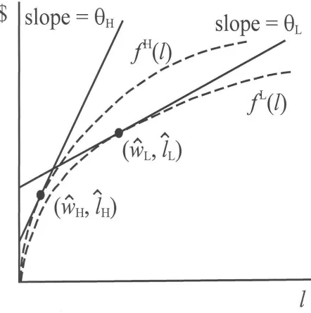
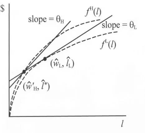
Please refer to Figure 1 for a graphical depiction of the equilibrium contracts with nonbindingICL, and Figure 2 for the case whenICLbinds. In these pictures,
the horizontal axis represents labor supply whereas the vertical axis represents
[image:16.612.194.415.433.655.2]wage, output or numéraire. Only the separating equilibrium where …rms can
Figure 2: Separating equilibrium, ICL binding
distinguish worker types exist.
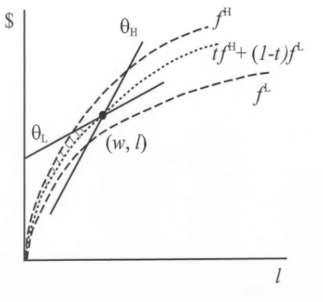
Figure 3 illustrates why a pooling equilibrium cannot exist. De…ne t =
NH=(NH +NL). The di¢culty with a pooling equilibrium lies in the …rms’ ability
to propose a deviating separating contract that attracts only the more productive
(type H) workers. It is always possible to pro…t from deviating to a separating
contract with typeH workers. Such contracts are represented by the shaded area
in Figure 3.
Worker types are identi…ed by their contract choices in the market. Types will not be pooled together at the same contract. Yet in a spatial setting, there is another kind of integration. Worker types can be integrated in a region or they
can be sorted between two regions.15 In the next subsection we distinguish by
their stability properties these two types of separating equilibria.
3.2
Stability properties of separating equilibria
Suppose a separating equilibrium has population distribution (^n1
H;n^1L;n^2H;n^2L):
Letsj =
b
njH= nbjH +bnjL be the high type share of regionj. There are two kinds of
15Note that “sorted by location” only refers to mobile workers. There are always immobile
Figure 3: Nonexistence of pooling equilibrium
separating equilibria: asorted separating equilibrium has only one type of worker in each region, i.e., sj 2 f1;0g , whereas an integrated separating equilibrium has
at least one region containing a mixture of the two types, i.e., 0 < s1 < 1 or
0< s2 <1. We examine their stability as follows.
Proposition 3.
(i) A sorted separating equilibrium with nonbinding ICL is always stable.
(ii) A sorted separating equilibrium with binding ICL is never stable.
(iii) An integrated separating equilibrium with either a binding or a nonbinding
ICL is stable if and only if
sj + 1 sj (s
j + 1 sj)
sj
H + (1 sj) L
1
L
(sj + 1 sj)
sj
H + (1 sj) L
1 1
L
1
+ L L
1 1
0; j = 1;2:
(iv) Fixing other parameters except for ,there are critical values1> s( )>0
and (sj) > 1 such that any integrated separating equilibrium with regional high
type shares s1; s2 > 0 is unstable: a) if min [s1; s2] < s( ), b) if and only if
Proof. See the Appendix.
The key intuitions and implications of this result are as follows. For the pur-pose of simulations, we shall focus on the case of a nonbinding ICL. An entering
…rm makes an o¤er to a perturbed worker before observing labor supply or type, based on population proportions of types in the region of origin at equilibrium. Risk neutrality on the part of …rms leads to their use of average production func-tions and average disutility of labor. Thus, an entering …rm o¤ers a deviating contract that maximizes expected pro…t under the average slope of the high and
low type production functions and the average disutility of labor , where the
average is taken according to the population of types in the region of origin at
equilibrium. Furthermore, competition drives …rms’ pro…t to zero. Stability
analysis employs disequilibrium behavior of …rms and workers, in contrast with the equilibrium contracting behavior studied in section 3.1.
The sorted separating equilibrium is always immune to a perturbation of work-ers since all agents are fully informed, so contracts are …rst best. Firms will not o¤er a better contract to attract moving workers. In contrast, when a mixture of workers of di¤erent types is moved to another region, a …rm entering in the destination region will o¤er a contract based on its expectations. This may give the low type a contract better than the equilibrium contract, for the following reason. Consider an integrated separating equilibrium. When the share of the high type in total mobile population is large so that the deviating contract is very close to the high type equilibrium contract, it is not attractive to the low type. This is because the high type equilibrium contract is not attractive to the low
type by condition ICL. So an integrated separating equilibrium can be stable.
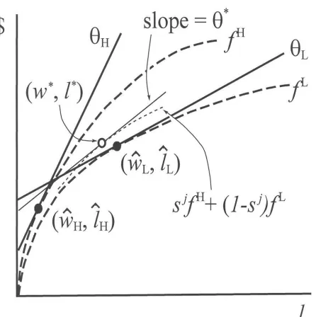
When the share of high type in total population is small enough, an entering …rm
will o¤er a more attractive contract (w ; l ) to the low type. This renders the
integrated separating equilibria unstable (see the illustration in Figure 4). For
any given high type productivity , there is a critical regional high type share
s( ) such that, for any smaller shares, integration of types is unstable.
Higher creates a larger di¤erence between the productivity of the two types.
This allows entering …rms to o¤er a more attractive contract to the low type when integrated with the high type. Thus, when the productivity of the high type is
Figure 4: Unstable integration of types
productivity is relatively high, they will be unstable. For any …xed regional high type share s, there is a critical value of high type productivity, (s), such that
a larger means integration of types is unstable. We will illustrate numerically
these critical values next in Section 4.
4
Simulation results
In this section, we illustrate with numerical examples the qualitative e¤ects of two key parameters, the technological advantage of high type workers, , and the share of high type workers in the mobile population,t, on stable equilibria. The equilibrium contract of the low type is …xed by their preferences and production
function. The following parameter values are used in the computations: = 0:4,
H = 1:2, L= 0:45.
4.1
Equilibrium
As takes a higher value, the high type production function becomes higher and
up. As a result, a high type worker enjoys a higher utility level. Table 1 shows a set of numerical results. Parameter takes values from1:1 to 1:2. VP and IC
conditions are satis…ed in this range. ICL binds for 1:201. To keep this
section simple, we only consider <1:201.
1 1:02 1:04 1:06 1:08 1:1 1:12 1:14 1:16 1:18 1:2
wH 0:481 0:497 0:513 0:530 0:547 0:564 0:581 0:598 0:616 0:633 0:651
lH 0:160 0:166 0:171 0:177 0:182 0:188 0:194 0:199 0:205 0:211 0:217
uH 0:288 0:298 0:308 0:318 0:328 0:338 0:348 0:359 0:369 0:380 0:391
Table 1
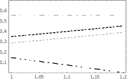
See Figure 5 for a graphical representation. Parameter is graphed on the
horizontal axis, whereas the values of the inequality constraints are on the vertical axis. Nonnegative values mean that the constraints are satis…ed. VP: thin, IC:
thick, type H: dotted, type L: dashed. When exceeds 1:201, ICL binds,
im-plying that the low skill type will be indi¤erent between the equilibrium contracts for low and high skill types.
1 1.05 1.1 1.15 1.2 0.1
[image:21.612.179.434.394.556.2]0.2 0.3 0.4 0.5 0.6
Figure 5: IC and VP conditions as a function of
4.2
Stability
of the high type share and the technological advantage parameter for which in-tegrating separating equilibria are not stable. We analyze the parameter range where all integrated separating equilibria are unstable for all possible regional high type shares. It is convenient to use the highest of the two regional high type shares, and compare the highest high type share to the critical share. Recall thatt=NH=(NH +NL)is the economy-wide share of the total high type mobile
population in the total mobile population. Actually, this share t is the highest
value of the minimum high skill share of the two regional shares:
t= max n1
H+n2H=NH;n1L+n2L=NL
min[ n
1
H
n1
H +n1L
; n
2
H
n2
H +n2L ]:
If one region has a high type share higher than t, the other region must have a
share lower than t. Thus, the task is reduced to …nding the critical high type
share in total population t such that, if t < t, then any integrated separating equilibrium is unstable.
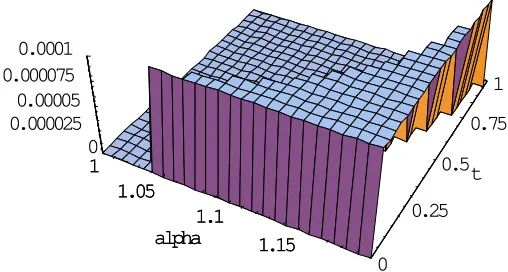
For a …xed t share, there is a critical value such that any integrated
equi-librium is unstable for > . Pairs of critical ( ; t) constitute a critical curve
that separates the parameter space into two parts. For values above ort values
below the critical curve, no equilibrium with integration of types is stable. The bene…t of a deviating contract for the low type (utility from a deviating contract minus utility from the equilibrium contract) is presented in Figure 6 (a positive value means integration-of-types is unstable).
A set of critical values ( ; t) are reported in Table 2.
1 1:02 1:04 1:06 1:08 1:1 1:12 1:14 1:16 1:18 1:2
t 0 0:023 0:050 0:081 0:117 0:162 0:218 0:290 0:392 0:555 0:944
Table 2
With immobile low skill workers in the background, as more are released to become mobile, t shrinks and eventually only sorted separating equilibria are
sta-ble. When the technological advantage of the high type increases, the integrated
1 1.05
1.1
1.15 alpha
0 0.25
0.5 0.75
1
t 0
0.000025 0.00005 0.000075
0.0001
1 1.05
1.1
[image:23.612.177.431.146.282.2]1.15 alpha
Figure 6: Unstable range for type integration
4.3
Transition of Stable Equilibria
We illustrate the transition of stable equilibria using a concentration index =
s1 s2 2[ 1;1]. The index represents the degree to which typeH workers are
concentrated in region 1 relative to region 2. When = 1, all type H workers
are in region 2. When = 0, both regions have the same share of typeH. When
= 1, all typeH workers are in region 1. A larger means a higher share of type
H workers in region 1 relative to the share in region 2.
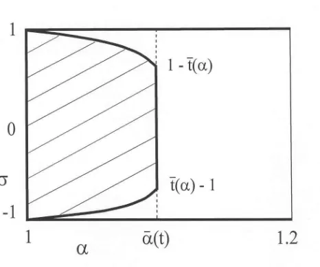
We can now evaluate at equilibrium for changing parameters and t.16
When t is …xed and the technological advantage parameter increases from 1,
integration of types is stable for middle ranges of . In Figure 7, the shaded area
represents the values of pairs of the productivity parameter and the
concentra-tion index such that the associated integrated separating equilibrium is stable.
This range is diminishing as is larger. When passes the critical (t), any
equi-librium with integration of types is unstable. Then only the sorted separating
equilibrium is stable, and we have agglomeration. Thus,sorted agglomeration can
16Let N1 =n1
1+n12 and N2 =n21+n22. For a given high type share in total population t,
any regional share combinations s1; s2 can be supported as a separating equilibrium (sorted
or integrated) if the following condition is satis…ed: s1N1+s2N2=t N1+N2 . Among this
Figure 7: Transition over for …xedt
be caused by increased productivity of high skill workers. For example, ift = 0:29, the critical = 1:14.
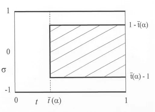
When is …xed and the high type share in total population t varies, we
represent equilibria in Figure 8. The shaded area represents pairs of high type
share t and concentration index such that the associated integrated separating
equilibrium is stable. For a large high type sharet, integration of types is is stable for intermediate values of . As more low types become mobile,tdecreases and for
t t( ), no equilibrium with integration of types is stable. Then only the sorted
separating equilibrium is stable, and once again we have sorted agglomeration
caused by mobility of more low skill workers.
Another way to generate similar comparative statics is to start with parameters so thatICL is initially binding and the economy wide proportion of high types is
low, but then increase the productivity of low skill workers until ICL no longer
binds. The stable equilibrium can change from integrated to sorted, whereas the equilibrium allocation changes from second to …rst best.
5
Conclusion
Figure 8: Transition over t for …xed
is de…ned in a broad sense as a stable but unequal population distribution
be-tween regions. If this is a consequence of sorting agents by type, then we call
in the agglomeration of workers by type. So,given asymmetric information in the labor market, either increased mobility of low skill workers or increased productiv-ity of high skill workers can result in separate agglomeration of workers by type,
consistent with the Berry and Glaeser (2005) work on human capital di¤erences between cities or the Combeset al (2006) work on wage dispersion across cities.
Extensions of the model include the following. First, land markets can be
added and the functional form assumptions can be generalized. We expect similar
results. In its current form, the transition to agglomeration is abrupt, as in
early models of the New Economic Geography. We expect that, analogous to
those models, the addition of land or amenities to our sparse model could smooth
the transition. Our functional forms were chosen so that the model is easy to
solve analytically. The cost of other functional forms would be more complex
calculations; the cost of general functional forms could be no method to solve the model analytically.
The model could be extended to include more regions and more types of
con-sumers (in particular, a continuum of types). More generally, heterogeneity of
…rms could be added. If …rm types were common knowledge, then the results
would likely be straightforward and similar. But if …rm types were private infor-mation, that would complicate the model substantially, since there would be two sided uncertainty in the labor market.
Extensions involving multiple periods and dynamic information revelation are
possible but are likely di¢cult. In communities with small populations, our
model might not be relevant because the type of a particular worker could be easily observable.
Further questions to be addressed include welfare properties of equilibrium al-locations and testable implications. Evidently, in the case of nonbinding incentive constraints, the equilibrium will be …rst best, but when an incentive constraint
binds, the equilibrium will generally be second best. We have presented some
comparative statics that might serve as testable implications. In particular, it
is evident from our pictures that high skill workers receive a higher average wage than low skill workers, so one can look for increasing wage dispersion for cities in a country over time, or larger wage dispersion for cities in developed countries in contrast with cities in developing countries.17
17A more direct approach, suggested by Bob Hunt, is to examine the extent of geographic
6
Appendix: Formal De…nition of a Consistent
Contract Structure and Proofs
De…nition of a Consistent Contract Structure:
Letn denote set subtraction. A contract structure (M;w;^ ^l;d^) is called
con-sistent if d^ satis…es the following rules. Fix k 2 M. (i) If the contract
o¤ered by …rm k does not give either type as much utility as that o¤ered by
another …rm or the outside option, then it attracts no workers and pro…ts are zero: if k 2 Mn[(ICH \ V PH) [ (ICL \V PL)] then k(M;w;^ ^l) = 0. In
this case, d^(k) = (0;0;0;0). (ii) If …rm k o¤ers a contract that is taken by only one type of worker, then that …rm knows with certainty the type it at-tracts: if k 2 (V PH \ICH)n(ICL\V PL), then k(M;w;^ ^l) = H w^k;^lk and
^
d(k) = (1;0;0;0) (if the …rm is in region 1) or d^(k) = (0;0;1;0) (if the …rm is in region 2); if k 2(V PL\ICL)n(ICH \V PH), then k(M;w;^ ^l) = L w^k;^lk and
^
d(k) = (0;1;0;0) (if the …rm is in region 1) or d^(k) = (0;0;0;1) (if the …rm is in region 2). (iii) Consider the case where the contract o¤ered by the …rm optimizes the utility of both types of workers given the contract structure. Then it is possi-ble for a …rm to attract any pro…le of workers, leading to a pro…t correspondence. To avoid unnecessary complications, and as is standard in the literature on
mech-anism design, we select a pro…le. It is a discontinuous selection, but again we
will guess and verify equilibrium, so its continuity properties are not important. (iii.a) If k 2 ICH \V PH \ICL\V PL and ([ICH \V PH)]n[ICL\V PL]) = 0
and ([ICL \ V PL]n[ICH \V PH]) = 0, then k(M;w;^ ^l) = NNH
H+NLf
H ^lk +
NL
NH+NLf
L ^lk w^k and d^(k) = ( NH
NH+NL;
NL
NH+NL;0;0) (if the …rm is in region 1)
or d^(k) = (0;0; NH
NH+NL;
NL
NH+NL) (if the …rm is in region 2). That is, when the
…rms o¤ering contracts that optimize utility for the high and low types are the same, then a …rm in this set can expect the economy-wide distribution of workers. (iii.b) If k 2 ICH \V PH \ICL\V PL and ([ICH \V PH)]n[ICL\V PL]) = 0
and ([ICL\V PL]n[ICH \V PH]) > 0, then k(M;w;^ ^l) = H w^k;^lk and set ^
d(k) = (1;0;0;0) if the …rm is in region 1 or d^(k) = (0;0;1;0) if the …rm is in region 2. That is, if a …rm o¤ers a contract that optimizes utility for both types of workers, but contracts are o¤ered by other …rms that are as good for the low type but not as good for the high type, then the …rm expects only high types.
Similarly, ifk 2ICH\V PH\ICL\V PLand ([ICH\V PH)]n[ICL\V PL])>0
and ([ICL \ V PL]n[ICH \ V PH]) = 0, then k(M;w;^ ^l) = L w^k;^lk and ^
d(k) = (0;1;0;0) (if the …rm is in region 1) or d^(k) = (0;0;0;1) (if the …rm is in region 2). (iii.c) Finally, if a …rm o¤ers a contract that optimizes utility for both types of workers but other …rms o¤er contracts that are as good for only the low type, whereas yet other …rms o¤er contracts that are as good only for the high type, then the …rm expects to get the economy-wide mixture of work-ers: if k 2 ICH \V PH \ICL\V PL and ([ICH \V PH)]n[ICL\ V PL]) > 0
and ([ICL \ V PL]n[ICH \V PH]) > 0, then k(M;w;^ ^l) = NHN+HNLfH ^lk + NL
NH+NLf
L ^lk w^k and d^(k) = ( NH
NH+NL;
NL
NH+NL;0;0) (if the …rm is in region 1)
or d^(k) = (0;0; NH
NH+NL;
NL
NH+NL)(if the …rm is in region 2).
18
Proposition 1. The following hold in equilibrium:
(i) V PH and V PL do not bind.
(ii) There is only one contract for each type of worker across locations and …rms.
(iii) If ICL (respectively, ICH) does not bind, fH (respectively fL) is tangent
to a type H (respectively type L) indi¤erence curve at the equilibrium contract. (iv) In a separating equilibrium, ICH does not bind.
Proof . (i) Suppose a typeH worker accepts an equilibrium contract (w0; l0)6=
(0;0) with uH(w0; l0) = 0. Thus, w0 = Hl0. By zero pro…t, fH(l0) =w0 and by
concavity d
dlf
H(l0)<
H. We can …nd a new contract(w00; l00)by reducing the labor
supply required by" <0, so thatl00 =l0 "andw00 =w0
H". This new contract
gives the worker the same utility (implying ICH) but increases the …rm’s pro…t.
Note that(w0; l0)satis…esIC
L anduL(w00; l00) =w0 Ll0+ L" H" < uL(w0; l0),
so(w00; l00)satis…es IC
L. These arguments apply to type L as well.
(ii) We prove this for the two types separately. First, suppose there are two distinct contracts (w1; l1) and (w2; l2) o¤ered to type H in equilibrium, and
uH (w1; l1) = uH(w2; l2). There are three possibilities: both …rms are certain
about worker types and use fH, both …rms are uncertain about worker types and
use the expected production function NH
NH+NLf
H( )+ NL
NH+NLf
L( ), or one …rm uses
18Since such stategies are never pro…table, we could also assume that the …rm attracts no
fH and the other uses the expected production function.
Case 1: two …rms use fH. By zero pro…t, fH(w
1; l1) = fH(w2; l2) = 0.
There is a new contract ((w1+w2)=2;(l1+l2)=2) that is indi¤erent for type H
(implyingICH) and yields more pro…t. The new contract satis…esICL since both (w1; l1) and (w2; l2)satisfy ICL.
Case 2 can be argued the same way as Case 1.
Case 3: One …rm usesfH and the other uses the expected production function.
Using zero pro…t, it must be thatfH(l
1) =w1, NHN+HNLfH(l2)+NHN+LNLfL(l2) = w2
and fH(l
2)> w2. There is a new contract (w1+ H"; l1 +") for small" >0 such
that it is indi¤erent for type H (implying ICH), attracts only type H workers,
and increases pro…t. It also satis…es ICL.
Second, suppose there are two distinct contracts (w1; l1) and (w2; l2)accepted
by type L in equilibrium. There are three possibilities: both …rms use fL, both
…rms use the expected production function NH
NH+NLf
H( ) + NL
NH+NLf
L( ), or one
…rm usesfL and the other uses the expected production function.
Cases 1 and 2 can be argued in the same way as Case 1 for type H.
Case 3: Using zero pro…t, it must be that NH
NH+NLf
H(l
1) +NHN+LNLfL(l1) =w1,
fH(l
2) = w2 and thusNHN+HNLfH(l2)+NHN+LNLfL(l2)> w2. There is a new contract
(w1+ H"; l1+") for small " >0 such that it is indi¤erent for type L (implying
ICL) and increases pro…t. It also satis…es ICH since both (w1; l1) and (w2; l2)
satisfyICH.
(iii) Suppose type H workers accept an equilibrium contract (w0; l0) (this is
unique by property (ii) and nonzero by property (i)) and ICL does not bind.
There is a small " >0such that contracts(w0+
H"; l0+")and (w0 H"; l0 ")
violate none of the VP or IC conditions. If d dlf
H(l0)>
H, the …rm can pro…tably
deviate to contract (w0+
H"; l0+"). If dldfH(l0) < H, the …rm can pro…tably
deviate to (w0
H"; l0 "). So, dldfH(l0) = H. The tangency condition can be
proved in the same way for type L workers and ICH.
(iv) Due to the single crossing property and property (ii), given thatICLbinds,
ICH also binds in and only in a pooling equilibrium. Since we are considering
only separating equilibrium, ICL does not bind. Suppose we have a separating
equilibrium with contract(w1; l1)for typeH and (w2; l2)for typeLand ICL does
not bind. Therefore, a …rm hiring a type H worker has the tangency condition:
fH(w
1; l1) = H (by property (iii)). By the concavity of the production functions,
bind sincew2 =fL(l2) by the zero pro…t condition.
Proposition 2.
(i) In a separating equilibrium, type L workers receive contract w^L;^lL =
L 1 ; L 1 1
. Type Hworkers receive contract w^H;^lH =
H 1 ; H 1 1
when ^l 1 H so ICLdoes not bind, and contract w^H0 ;^l = w^L L ^lL ^l ;^l
when ^l 1 > H and ICL binds, where ^l is the solution to
L^l ^l + L 1 L L 1 1
= 0:
(ii) Workers reveal their types in equilibrium. In other words, there is no pooling equilibrium.
Proof. (i) We construct the unique separating equilibrium contracts by utilizing
results in Proposition 1. First, since ICH does not bind, the low type is always
o¤ered a contract at a tangency. Suppose a …rm hires a type L worker with
contract (wL; lL). By zero pro…t, (lL) wL = 0 and by tangency of the type L
production function and the typeLindi¤erence curve, dldfL(lL) = (lL) 1 = L.
The equilibrium contract is
^lL= L
1 1
;w^L = L
1
:
By the concavity offL, w
L LlL>0 and V PL is satis…ed.
Second, since uL w^L;^lL > 0 and fH ^lL > fL ^lL = ^wL, this particular
indi¤erence curve passing through w^L;^lL intersectsfH at a point w ;^ ^l such
that^l <^lL. This ^l can be solved from zero pro…t:
fH ^l = ^w
L L ^lL ^l ;
or
L^l ^l +
1
L
1 1
If d dlf
H ^l
H, or
^
l 1 H;
then type H can achieve a higher payo¤ than w ;^ ^l at a contract w^H;^lH
such that ^lH ^l. This is solved from zero pro…t, (lH) wH = 0, and the
tangency of the type H production function and the type H indi¤erence curve:
d dlf
H(l
H) = (lH) 1 = H. Therefore,
^lH = H
1 1
;w^H =
H
1
:
By the concavity of production functions, V PH,ICH and ICL are all satis…ed.
Third, if d
dlf
H ^l >
H, then w ;^ ^l is the highest payo¤ type H can
get under zero pro…t and ICL, since ICL binds. Note that V PH is satis…ed
by concavity whereas ICH is satis…ed due to the slope di¤erence, H > L, of
indi¤erence curves.
To this point of the proof, we have used necessary conditions for equilibrium
contracts to solve for them. To prove formally that these are equilibrium
con-tracts, we must show that there are no independent, pro…table …rm deviations.
This can easily be seen, for example, using Figures 1 and 2. Any alternative
contract o¤ered by a …rm will yield negative pro…t, or will violate an incentive or production constraint.
(ii) Suppose there is a nontrivial pooling contract(w; l)6= (0;0)in the market that both types of workers accept with a high type share NH
NH+NL. If a …rm can o¤er
a di¤erent contract arbitrarily close to (w; l)that attracts typeH workers but not
type L workers, it can use production function fH instead of the average of two
production functions. This brings more pro…t since the increase in production is a discontinuous jump. A contract (w L"; l ") for small " > 0is that kind of
deviating contract. A type H worker is indi¤erent between the deviating contract
and (w; l), while a type L worker prefers (w; l), since uL(w H"; l ") = w
Ll+ ( L H)" < uL(w; l).
Proposition 3.
(i) A sorted separating equilibrium with nonbinding ICL is always stable.
(iii) An integrated separating equilibrium with either a binding or a nonbinding
ICL is stable if and only if
sj + 1 sj (sj + 1 sj)
sj
H + (1 sj) L
1
L
(sj + 1 sj)
sj
H + (1 sj) L
1 1
L
1
+ L L
1 1
0; j = 1;2:
(iv) Fixing other parameters except for ,there are critical values1> s( )>0
and (sj) > 1 such that any integrated separating equilibrium with regional high
type shares s1; s2 > 0 is unstable: a) if min [s1; s2] < s( ), b) if and only if
>min [( (s1); (s2)].
Proof.
(i) Sorted separating equilibrium with nonbindingICL:
When the two types of workers are sorted by location in a separating equilib-rium, …rms know for sure the type of a worker coming from a particular region. All agents are fully informed. Thus, when a worker moves to another region, an entering …rm o¤ers a …rst best contract that yields zero pro…t. This contract turns out to be that same …rst best contract that the worker receives in equilibrium.
(ii) Sorted separating equilibrium with bindingICL:
In equilibrium, the contract for the high type is second best. When a high type worker is perturbed, an entering …rm o¤ers the …rst best contract. Instability is the direct result of the incentive constraint binding.
(iii) Integrated separating equilibrium with a nonbinding ICL:
The stability of an integrated separating equilibrium depends on the compo-sition of its worker populations. When a small measure of workers is moved from regionj to the other region, the …rms hiring the perturbed workers have expected output
sjfH(l) + 1 sj fL(l):
Since the workers cannot be distinguished, …rms will pay a uniform wage rate to all workers that equals the expected disutility of labor
Pro…t maximization determines the quantity of labor hiredl :
d dl s
j
fH(l ) + 1 sj fL(l ) = :
This means
l = (s
j + (1 sj)) 11
:
By competition, the …rm will o¤er a total wagew at zero pro…t.
w = sj + 1 sj (l ) ;
= sj + 1 sj (s
j + (1 sj))
sj
H + (1 sj) L
1
:
This contract (w ; l ) is below the fH production function and will not be
accepted by type H workers. Type L workers will accept it if
w Ll >w^L L^lL; or
sj + 1 sj (s
j + 1 sj)
sj
H + (1 sj) L
1
L
(sj + 1 sj)
sj
H + (1 sj) L
1 1 > L 1 L L 1 1 :
Integrated separating equilibrium with a binding ICL:
Exactly the same calculations work whenICL binds, since the behavior of the
high type is irrelevant. To see this, please refer to Figure 2 and apply the single crossing property at the equilibrium contract for the high type,( ^w0
H;^l ). Notice
that if the perturbed high type workers want to stay in their new region, so do the low type workers. So the equilibrium is unstable only if the low type workers want to stay in the new region. Next, notice that if the low type workers want to stay in their new region, then the equilibrium is unstable by de…nition. Hence, the equilibrium is unstable if and only if the low type workers want to stay in their new region, thus rendering the behavior of high types irrelevant, and reducing the
problem to the same one as with a nonbinding ICL.
(iv) Let
( ; s) = (s + 1 s) (s + 1 s)
s H + (1 s) L
1
L
(s + 1 s)
s H + (1 s) L
denote the utility level of a low type worker from a deviating contract and s is the high type share of the original region. Therefore, the contract is attractive if
( ; s)> ( ;0):
First, let ( ; s) = s(s +1 s)
H+(1 s) L.
@ ( ; s)
@s = ( 1) ( ( ; s))1 + (s + 1 s)1 ( ( ; s))
2 1
1 @ ( ; s)
@s
L
1 ( ( ; s))1
@ ( ; s)
@s ;
where
@ ( ; s)
@s =
( 1) (s H + (1 s) L) (s + 1 s) ( H L) (s H + (1 s) L)2
:
We have
( ;0) = L
;
@ ( ; s)
@s j s=0 =
( 1) L ( H L) ( L)2 :
This means
@ ( ; s)
@s j s=0 = ( 1) L
1
+
1 L
2 1
1 ( 1)
L ( H L) ( L)2
L
1 L
1 ( 1) L ( H L)
( L)2 ;
= ( 1) L
1
>0:
Therefore, ( ; s)> ( ;0)for allsclose enough to0. An integrated equilibrium is unstable if s1 ors2 is small enough.
Second, since
@ ( ; s)
@ =
s
s H + (1 s) L
@ ( ; s)
@ = s( ( ; s))1 + (s + 1 s)1 ( ( ; s))
2 1
1 d ( ; s)
d
L
1 ( ( ; s))1
d ( ; s)
d
= ( ( ; s))1 s+ s
1
Ls
(1 ) (s H + (1 s) L)
;
= ( ( ; s))1 s
1 1
L
s H + (1 s) L
:
We have, for alls >0,
@ ( ; s)
@ >0
because <1and L
s H+(1 s) L <1. Moreover, for …xeds >0,
@ ( ;s)
@ is increasing
in , and thus is bounded away from zero. Notice, however, that
@ ( ; s)
@ js=0= 0
We conclude that ( ; s)> ( ;0) if and only if is large enough.
References
[1] Abdel-Rahman, H., 1988, Product di¤erentiation, monopolistic competition and city size, Regional Science and Urban Economics 18, 69-86.
[2] Abdel-Rahman, H., 1990, Sharable inputs, product variety and city sizes, Journal of Regional Science 30, 359-374.
[3] Abdel-Rahman, H. and M. Fujita, 1990, Product variety, Marshallian exter-nalities, and city sizes, Journal of Regional Science 30, 165-183.
[4] Acemoglu, D., 1999, Changes in unemployment and wage inequality: An alternative theory and some evidence, American Economic Review 89, 1259-1278.
[5] Berman, E., J. Bound, Z. Griliches, 1994, Changes in the demand for skilled labor within U.S. manufacturing industries: Evidence from the annual survey of manufacturing, Quarterly Journal of Economics 108, 367-398.
[7] Blum, B., Bacolod, M. and W. Strange, 2006, Hard skills, soft skills and
agglomeration: A hedonic approach to the urban wage premium. Paper
presented at the 53rd Annual North American Meetings of the Regional Sci-ence Association International in Toronto.
[8] Caselli, F. 1999, Technological revolutions, American Economic Review 89, 78-102.
[9] Combes, P.-P., Duranton, G. and L. Gobillon, 2006, Spatial wage disparities: Sorting matters!, working paper.
[10] Ellison, G. and E. Glaeser, 1997, Geographic concentration of U.S. manufac-turing industries: A dartboard approach, Journal of Political Economy 105, 889-927.
[11] Ellison, G. and E. Glaeser, 1999, The geographic concentration of industry: Does natural advantage explain agglomeration?, American Economic Review 89, 311-316.
[12] Fang, H., 2001, Social culture and economic performance, American Eco-nomic Review 91, 924-937.
[13] Fujita, M., 1986. Urban land use theory, in Location Theory. Edited by J. Lesourne and H. Sonnenschein. New York: Harwood Academic Publishers.
[14] Fujita, M., 1988, A monopolistic competition model of spatial agglomeration: Di¤erentiated product approach, Regional Science and Urban Economics 18, 87-124.
[15] Fujita, M. and Thisse, J.-F., 2002, Economics of Agglomeration. Cambridge: Cambridge University Press.
[16] Hunt, R.M., 2005, A century of consumer credit reporting in America, Work-ing paper no. 05-13, Research Department, Federal Reserve Bank of Philadel-phia.
[17] Konishi, H., 2006, Tiebout’s Tale in Spatial Economies: Entrepreneurship, Self-Selection, and E¢ciency. http://fmwww.bc.edu/EC-P/WP655.pdf
[19] Starrett, D. 1978, Market allocations of location choice in a model with free mobility, Journal of Economic Theory 17, 21-37.
[20] U.S. Department of Commerce, 1975, Historical Statistics of the United
States: Colonial Times to 1970 Part 1. Washington, DC: Bureau of the