Comparative Study of Different Representations in Genetic Algorithms for Job Shop Scheduling Problem

(1)

http://dx.doi.org/10.4236/jsea.2014.77053

How to cite this paper: Jorapur, V., Puranik, V.S., Deshpande, A.S. and Sharma, M.R. (2014) Comparative Study of Different Representations in Genetic Algorithms for Job Shop Scheduling Problem. Journal of Software Engineering and Applications, 7, 571-580. http://dx.doi.org/10.4236/jsea.2014.77053

Comparative Study of Different

Representations in Genetic Algorithms

for Job Shop Scheduling Problem

Vedavyasrao Jorapur

*

, V. S. Puranik, A. S. Deshpande, M. R. Sharma

Visvesvaraya Technological University, Belgaum, India Email: *[email protected]

Received 13 February 2014; revised 10 March 2014; accepted 18 March 2014

This work is licensed under the Creative Commons Attribution International License (CC BY). http://creativecommons.org/licenses/by/4.0/

Abstract

Due to NP-Hard nature of the Job Shop Scheduling Problems (JSP), exact methods fail to provide the optimal solutions in quite reasonable computational time. Due to this nature of the problem, so many heuristics and meta-heuristics have been proposed in the past to get optimal or near-op- timal solutions for easy to tough JSP instances in lesser computational time compared to exact methods. One of such heuristics is genetic algorithm (GA). Representations in GA will have a direct impact on computational time it takes in providing optimal or near optimal solutions. Different representation schemes are possible in case of Job Scheduling Problems. These schemes in turn will have a higher impact on the performance of GA. It is intended to show through this paper, how these representations will perform, by a comparative analysis based on average deviation, evolu- tion of solution over entire generations etc.

Keywords

Job Shop Scheduling, Genetic Algorithm, Genetic Representation, Conceptual Model

1. Introduction

Scheduling is a decision-making process which deals with allocation of resources to tasks over given time-pe- riods and its goal is to optimize one or more objective functions. A scheduling problem is represented by triplet α/β/γ.α field describes machine environment; β field provides details of processing characteristics and constraints and γ field describes the objective function to be minimized. Being essentially a combinatorial optimiza-tion problem, job shop scheduling has caught the attenoptimiza-tion of researchers in the last so many years for optimized

(2)

performance. Combinatorial optimization problems can be classified as easy and hard. Problems which are poly- nomialy solvable with limited number of variables are treated easy and are called P. The notion polynomial solvable depends on the type of encoding. It is assumed that problems describing numerical data are binary en-coded and the number of steps involved in solving these increases exponentially with increase in length of string and hence computational time will be enormously large and treated to be hard problems. Job scheduling prob-lems belong to this category and are termed NP-Hard [1]. In the practical manufacturing environment, the scale of job shops is generally much larger than that of JSSP bench mark instances considered in theoretical research. Optimization algorithms for job shop scheduling usually proceed by Branch and Bound and among the most re- cent and successful, ones are those of Carlier and Pinson (1989) and Applegate and Cook (1991) [2]. Approxi-mation procedures or heuristics were initially developed on the basis of priority rules or dispatching rules. The quality of solutions generated by these procedures leave plenty of room for improvement (1998) [3]. Therefore, traditional or meta-heuristic algorithms can hardly be able to solve such problems satisfactorily. In manufacturing workshops, availability of computational resources is much less than the laboratories which lead to difficulty in exploring all possible feasible solutions. Under such circumstances, it is reasonable to reduce the search space and range to only promising areas. The very idea of using constructive heuristics and heuristic search algorithms for larger problem sizes of JSSP is the computational expensive nature of enumerative techniques and Lagrann- gian algorithms. According to Osman (1996), a heuristic search “is an iterative generation process which guides a subordinate heuristic by combining intelligently different concepts for exploring and exploiting the search spaces”.

Extensive use of genetic algorithms to solve job shop scheduling problems can be seen through literature survey [4]. However, how effectively genetic algorithms can be used in JSSP case is not completely explored. In this context, some direction is provided by Tamer F. Abdelmaguid [5] in his paper. Ga’s are based on an abstract model of natural evolution, such that quality of individuals builds to the highest level compatible with the environment (constraints of the problem). (Holland, 1975; Goldberg, 1989)

Representations in GA environment applied so far in job shop scheduling can be classified into nine categories as given by Cheng et al. (1996):

1) Operation based 2) Job based 3) Job pair relation based 4) Completion time based 5) Random keys 6) Preference list based 7) Priority rule based 8) Disjunctive graph based. 9) Machine based.

Nine categories mentioned above can be grouped into two basic encoding approaches—direct and indirect encoding. In direct approach, a Πj schedule is encoded as a chromosome and genetic operators are used to evolve better individual ones. Categories 1 to 5 are examples of this category. In case of indirect approach, a sequence of decision preferences will be encoded into a chromosome. In this, encoding, genetic operators are applied to improve the ordering of various preferences and a Πj schedule is then generated from the sequence of preferences. Categories 6 to 9 are examples of this category [6]. These representations need to be studied in case of job shop scheduling problems to compare their performance criteria to generate optimal or near optimal solutions, even though computational comparison of different representations is reported in a tutorial paper by Cheng, Gen and Tsujimura [6]. A report by Anderson, Glass and Potts [7], conducted with different metaheu- ristics approaches including four different GA implementations, lacks in consistency as well as coherence as re- gards number of test problems being tested with requisite number of runs.

The rest of this paper is organized as follows: We will start with mathematical models with certain assumptions that have been used in next section followed by the literature review on the different GA representations used in the case of JSP. Followed by review of GA representations, we will discuss regarding different GA operators frequently used by researchers and our own views on adding other operators not discussed so far. Now, we will analyze the experimental results conducted followed by the conclusion provided in the final part of this paper.

2. Problem Formulation

Since it is an important practical problem, some authors have formulated various JSP models based on different production situations and problem assumptions. The most common assumptions in case of JSP are:

1) A machine may process more than one job at a time;

(3)

3) The sequence of machines which a job visits is completely specified and has a linear precedence structure; 4) Processing times are known. All the processing times are assumed to be integers;

5) Each job must be processed on each machine only once. There is no recirculation; 6) Set-up times are assumed zero;

7) Pre-emption is not allowed.

Let “J” represent a set of jobs and each job will be processed on a set of machines in a particular order. Let I = (1…..v) represent the operation indexes. The operation indexes are assigned such that for a job k∈ J, the subset of consecutive indexes I_k = β β_k, _k+1,β_k+2,ω_k ⊆I, is a subset containing indexes for that job. Now from the subset Ik depending on the priority operation with higher or lower value is processed first. Let pi be the

processing time of ith operation, the job which it belongs to is j(i) and the machine on which ith operation carried is m(i).

Now the objective of scheduling process is to determine the start time sti of an operation i∈ I. While assign- ing a job to a machine based on above calculations following constraints should be taken into consideration viz. The technological constraints will take care of order of operations to be carried out on a job and a second set of constraint will take care of conflict of two jobs to be processed on the same machine simultaneously. Accor- dingly:

1.. Is the equation to satisfy technological constraints

i i i

st +p ≤st+ (1)

and

Or

i j j j i i

st ≥st +p st ≥st +p (2)

Is the equation to satisfy the conflict of two jobs on the same machine at the same time.

( )

, I where and

i j m i m j j i j j

∀ ∈ = ≠

Different total cost functions that can be studied are

( )

{

( )

}

. : . 1, ,

max i i

F C =max f C i=  n …Is called Bottleneck objective and

( )

1

i n

i i i

i

f C f C

=

∑

… Is called Sum Objective.

The most common objective functions are the make span max

{

( )

Ci i=1,,n

}

and total flow time

( )

1 n i i C =

∑

, and weighted (total) flow time

1 n i i i w C = ⋅

∑

. We have considered the minimization of make span as our objective function. Mannes’ [8] proposed an integer linear programming model (ILP) which uses different forms of binary variables. This model has gained larger interest in the research community due to small number of variables considered in the model. The technological constraints of Equation (1) are analogous to a series of consecutive activities that are carried out in project scheduling. This analogy has motivated importing project networks into JSP environment. To represent disjunctive constraints as in Equation (2), additional sets of arcs required. This is achieved in a disjunctive graph model [9] and PIAN model [10].

In the disjunctive graph model, a disjunctive arc is defined between a pair of operations that share the machine. Each disjunctive arc is assigned a binary decision variable such that selection on the value that variable defines the length and direction of each disjunctive arc. This is to the Mannes’ model. Very efficient algorithms like immediate selections and shifting bottleneck heuristics were proposed by Carlier [11] and Adams [12]and Lars Monch [13], which are derived from disjunctive graph model.

A variable notation of the type

m i,t

x = 1…if operation ‘i’ is processed on machine ‘m’ in unit time ‘t’ = 0...otherwise.

In ILP model was proposed by Bowman [14]. Wagner [15] proposed a model where a variable notation of the type: xm_i,l = 1…if operation ‘i’ takes ‘ith’ position in the processing sequence on machine ‘m’

= 0...otherwise.

And. Mannes’ [8] proposed a model where a variable notation of the type: xm_i,j = 1…if operation ‘i’ is processed prior to operation ‘j’ on machine m.

(4)

3. Representation of the Problem in GA and GA Operators

Darwin’s principle “survival of the fittest” can be used as a starting point in introducing evolutionary computa- tion. The problems of chaos, chance, non linear interactivities and temporality being solved by biological spe- cies are proved to be in equivalence with classic method of optimization [15].

Evolutionary computations techniques that contain algorithms based on evolutionary principles are used to search for an optimal or best possible solution for a given problem. In a search algorithm, number of possible solutions is available and the task is to find the best possible solution in a fixed amount of time. Traditional search algorithms randomly search (e.g. random walk) or heuristically search (e.g. gradient descent), explore one solution at a time in the search space to find best possible or optimal solution, which is computationally in- efficient as the search space grows in size. Whereas evolutionary algorithms from such traditional algorithms are population based. Evolutionary algorithm performs a directed efficient search by adaptation of successive generations of a larger number of individuals. Genetic Algorithms is one such evolutionary algorithm in finding an optimal or near optimal solution to a problem. In a traditional genetic algorithm, the representation is bit length string. Its approach is to generate a set of random solutions from the existing solutions, so that there is an improvement in the quality of solutions throughout the generations. This implementation is achieved through main GA operators’ viz. random selection of two solutions from individuals in the parent generation; performing crossover operation on these two solutions to generate two new child solutions. Crossover operation is per- formed by exchanging specific elements of the two solutions selected; and mutation operation is conducted on child solutions to further explore the search space for better solutions. Different variations in simple GA approach can be found in literature survey to improve its search capabilities [16]. Representation of solutions of an optimization problem is to be done in a suitable format in GA to deal with reproduction and mutation operators. This format or structure referred as genotype, needs to be easily interpretable to a solution of the problem under study. In a combinatorial optimization problem, representation of a solution in GA is difficult as well as a chal- lenging task. These are problems containing discrete decision variables and are interrelated by logical relation- ships. As a result, different mathematical models may exist for the same combinatorial optimization problem and this may lead to different representations for the same problem.

As explained above Cheng, Gen and Tsujimura [6] in their paper representation of JSP in GA into direct and indirect type. Further to that, T. F. Abdelmaguid [17] in his paper classified GA representations into Model based and Algorithm based. In our opinion, all representations are algorithm based though they appear to be model based.

In Priority Rule Based (PR) representation, a chromosome is represented as a string of (n − 1) entries (p1,

p2…pn) where n − 1 is the number of operations in the problem instance. An entry p1 represents a priority rule

selected beforehand. Accordingly, a conflict in the ith iteration of Giffler and Thompson algorithm [18] should be resolved using priority rule represented by pi. It means an operation from the conflict set has to be selected by the pi ties are broken randomly. In GA domain, a best set of priority rules should be selected. Here simple crossover yields feasible schedules.

In Random Keys Representation (RK) was first proposed by Bean [19]. In this representation, each gene is represented with random numbers generated between 0 and 1. These random numbers in a given chromosome are sorted out and are replaced by integers and now the resulting order is the order of operations in a chromosome. This string is then interpreted into a feasible schedule. Any violation of precedence constraints can be corrected by a correction algorithm incorporated.

In Operation based representation, each gene represents an operation. A chromosome contains as many genes as the number of operations. For example, an nx m JSP there will be nxm genes in the chromosome. Beirwirth proposed a technique “permutation with repetition” [20] which is similar to operation based representation. Fang [21] also proposed a kind operation based representation where string contains nxm chunks which are large enough to hold the largest job number for the nxm JSP. Whereas Beirwirth used a special GOX crossover technique to generate feasible schedule, Fang used a special decoding approach to decode a chromosome into a valid schedule always.

The Preference List based representation (PL) uses a string of operations for each machine instead of a single string for all operations which is a direct representation of processing sequence decision variables. Quite often violation of constraints is encountered which can be overcome by repair algorithm.

(5)

machine in the shifting bottleneck algorithm [12].

In the Job based representation[22] a chromosome is a string of length equal to the number of jobs in the problem under study. Using this representation, a simple algorithm can generate a feasible schedule given sequence of the jobs onto different machines.

4. Methodology

The reproduction and mutation operators applied to JSP model are generally adopted from Travelling Salesman Problem because of the similarity in representations. Reproduction operators are generally required in GA to conduct the neighborhood search and a mutation operator generally ensures that the solution is not trapped in local minima. The design of both operators is crucial for the success of GA. Among the reproduction operators reported in the literature, PMX (partially matched crossover) [23], OX (ordered crossover) [24] and uniform crossover [25] are extensively used in JSSP. PMX and OX crossover techniques use either single point or two point crossover. Different mutation operators used are swap mutation, inversion mutation and insertion or shift mutation reported in the literature [17].

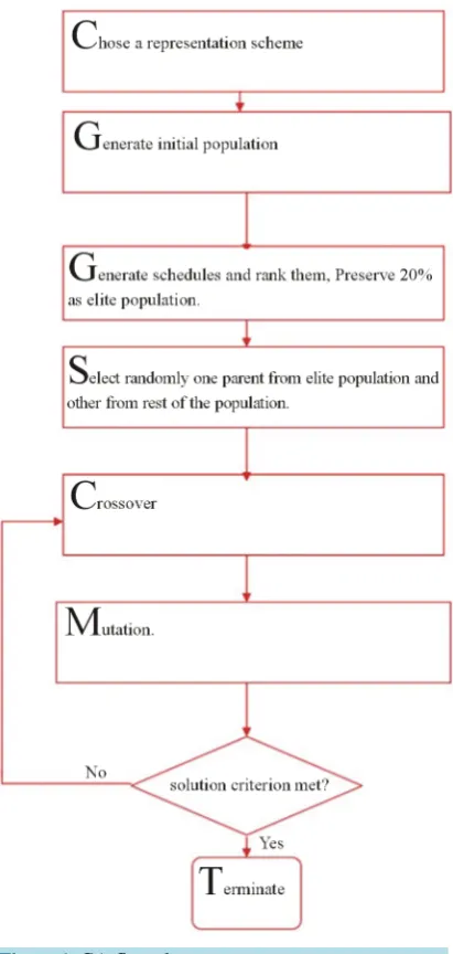
In general, the flow chart for GA can be represented as shown.

5. Results and Analysis

In our experiment, four representations are used viz. Operation based (OB), Job based (JB), Machine based (MB), Priority rule based (PR). All experiments are conducted with 50 generations and a population size of 1000. Mutation probability varies with 0.1 to 0.9 values dynamically and elite population size is 20%. Reproduction probability used in our experiment is 0.1 Parents in our experiment are selected from two groups sorted out based on fitness value (i.e. minimum make span). Each parent is selected from these groups probabilistically.

In our experimentation, GA is programmed with different reproduction and mutation operators’. Instead of selecting operators randomly as in [17], we have built-in reproduction operators and are being used across the representations and the benchmark instances. The benchmark problems used in this paper are taken from OR li- brary [26] available in World Wide Web. All the experiments are conducted with a Pentium-4 dual core proces- sor with clock speed of 2.06 GHz and RAM of 512 Mbs. 68 benchmark instances are taken and in the single run, the best and average values are obtained and compared with lower bound or optimum value of the benchmark instance. Results are shown in Table 1. Different graphs generated are also shown below.

Table 1.Results of benchmark instances under different representations.

Problem Size _OperationsNo. of Best Known _Solution OB OB JB JB MB MB PR PR

Best Avg. Best Avg. Best Avg. Best Avg.

mt06 6 × 6 36 55 55 64.889 55 65.712 55 61.822 55 66.648

mt10 10 × 10 100 971 989 1116.02 971 1100.9 992 1145.06 958 1100.42

mt20 5 × 20 100 1206 1220 1394.47 1206 1383.08 1245 1427.24 1242 1426.54

abz05 10 × 10 100 1259 1275 1394.79 1259 1386.12 1287 1409.87 1267 1390.94

abz06 10 × 10 100 971 958 1072.19 971 1075.97 996 1096.13 978 1080.3

abz07 15 × 20 300 742 734 821.16 742 804.892 751 817.937 730 807.128

abz08 15 × 20 300 758 751 833.362 758 825.982 763 838.59 755 826.954

abz09 15 × 20 300 752 784 877.468 752 849.838 773 873.541 764 859.258

car01 5 × 11 55 7038 7038 8747.84 7038 8694.01 7038 8707.83 7038 8782.28

car02 4 × 13 52 7376 7378 8788.38 7376 8738.23 7221 8817 7166 8881.94

car03 5 × 12 60 7725 7590 9219.19 7725 9195.36 7725 9293.86 7725 9272.51

car04 4 × 14 56 8072 8003 9620.16 8072 9452.62 8276 9697.21 8132 9643.3

car05 6 × 10 60 7835 7873 9207.14 7835 9130.26 7862 9251.68 7862 9407

car06 9 × 8 72 8505 8505 10017.7 8505 9886.82 8505 10229.5 8485 9830.33

car07 7 × 7 49 6558 6576 7673.64 6558 7782.76 6627 7751.89 6632 7738.75

car08 8 × 8 64 8407 8407 9436.29 8407 9500.61 8458 9470.57 8366 9470.64

(6)

Continued

la02 5 × 10 50 655 665 748.122 655 774.664 660 745.747 667 757.79

la03 5 × 10 50 617 620 688.729 617 687.389 626 690.773 620 699.527

la04 5 × 10 50 607 595 695.259 607 690.822 619 699.926 602 688.268

la05 5 × 10 50 593 593 640.494 593 658.885 593 606.404 593 699.114

la06 5 × 15 75 926 926 1000.79 926 1021.85 926 958.039 926 1075.5

la07 5 × 15 75 890 890 998.253 890 1015.05 893 983.784 890 994.044

la08 5 × 15 75 863 863 981.109 863 985.795 863 959.264 863 995.054

la09 5 × 15 75 951 951 1051.15 951 1084.34 951 988.331 951 1167.81

la10 5 × 15 75 958 958 1017.01 958 1045.73 958 971.19 958 1089.97

la11 5 × 20 100 1222 1222 1308.89 1222 1334.96 1222 1264.12 1222 1389.85

la12 5 × 20 100 1039 1039 1132.34 1039 1157.8 1039 1104.58 1039 1226.58

la13 5 × 20 100 1150 1150 1248.7 1150 1278.51 1150 1191.37 1150 1314.64

la14 5 × 20 100 1292 1292 1320.59 1292 1348.95 1292 1295.72 1292 1388.82

la15 5 × 20 100 1207 1207 1336.66 1207 1352.88 1227 1368.04 1207 1352.41

la16 10 × 10 100 979 982 1083.26 979 1066.88 988 1088.68 987 1071.61

la17 10 × 10 100 797 793 890.389 797 885.073 832 905.275 807 888.012

la18 10 × 10 100 861 861 962.052 861 967.819 885 976.877 883 977.685

la19 10 × 10 100 875 875 970.966 875 972.302 899 983.686 877 976.925

la20 10 × 10 100 936 907 1022.37 936 1040.62 944 1039.52 914 1041.05

la21 10 × 15 150 1105 1098 1252.76 1105 1247.82 1115 1264.74 1111 1281.85

la22 10 × 15 150 972 988 1146.21 972 1125.68 1031 1161.32 990 1133.83

la23 10 × 15 150 1035 1045 1188.52 1035 1168.18 1037 1180.52 1068 1187.63

la24 10 × 15 150 1004 1006 1135.91 1004 1134.02 1029 1155.7 995 1149.69

la25 10 × 15 150 1040 1055 1177.18 1040 1170.37 1036 1175.69 1058 1178.36

la26 10 × 20 200 1269 1279 1457.86 1269 1424.04 1304 1466.35 1310 1446.12

la27 10 × 20 200 1341 1363 1529.94 1341 1500.85 1421 1539.77 1374 1538.38

la28 10 × 20 200 1301 1295 1454.95 1301 1456.94 1334 1463.16 1284 1453.35

la29 10 × 20 200 1274 1302 1441.65 1274 1416.42 1307 1429.08 1270 1425.34

la30 10 × 20 200 1418 1429 1576.32 1418 1554.81 1444 1592.45 1432 1591.74

la31 10 × 30 300 1784 1784 1927.56 1784 1938.51 1785 1934.69 1784 1933.39

la32 10 × 30 300 1850 1850 2019.59 1850 2029.95 1855 2024.57 1853 2031.31

la33 10 × 30 300 1719 1725 1890.07 1719 1873.95 1719 1871.39 1725 1883.41

la34 10 × 30 300 1757 1782 1942.11 1757 1916.99 1801 1941.67 1793 1941.16

la35 10 × 30 300 1890 1905 2090.49 1890 2079.74 1919 2116.75 1906 2097.97

la36 15 × 15 225 1348 1343 1515.99 1348 1492.07 1385 1519.31 1352 1498.9

la37 15 × 15 225 1486 1506 1674.69 1486 1651.36 1548 1698.19 1496 1687.76

la38 15 × 15 225 1319 1307 1455.03 1319 1474.01 1369 1494.87 1299 1486.33

la39 15 × 15 225 1316 1325 1486.54 1316 1479.86 1383 1519.21 1363 1508.05

la40 15 × 15 225 1296 1330 1469.25 1296 1460.38 1360 1485.68 1338 1492.6

orb01 10 × 10 100 1124 1130 1262.1 1124 1277.16 1150 1304.67 1126 1277.02

orb02 10 × 10 100 924 919 1047.74 924 1031.34 949 1045 931 1060.46

orb03 10 × 10 100 1067 1116 1254.65 1067 1232.93 1080 1262.65 1065 1230.21

orb04 10 × 10 100 1028 1055 1176.34 1028 1154.35 1075 1164.81 1053 1160.75

orb05 10 × 10 100 931 945 1075.54 931 1056.76 969 1109.28 931 1064.55

orb06 10 × 10 100 1046 1093 1248.37 1046 1213.47 1116 1272.66 1067 1233.12

orb07 10 × 10 100 419 415 469.22 419 467.724 425 472.424 418 470.205

orb08 10 × 10 100 928 940 1113.01 928 1075.88 969 1135.78 947 1102.29

orb09 10 × 10 100 949 953 1080.08 949 1059.32 958 1066.74 964 1079.28

(7)

[image:7.595.211.417.280.713.2]

6. Conclusion & Future Scope

Figure 1 shows a plot of % deviations of different instances from the Lower Bound values or Optimum values vs. different representations in GA. It is clear that all representations, across the benchmark instances have shown nearly similar deviations. It is quite clear from the graph that Job Based representations have shown con- siderable lower peaks. This shows that with the use of proper local search technique it is possible to find the optimal solution.

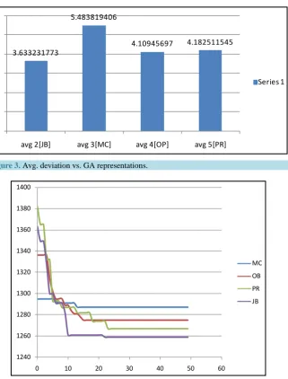
Figure 2 and Figure3 show a plot of average deviations of different representations. Except Machine based all other representations have shown the similar deviation. We conclude from this plot that Machine based representation performance is poor and Job based representation performance is better.

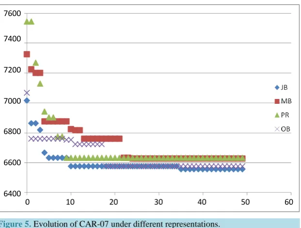
The evolution process over 50 generations for the benchmark instance ABZ 5 for instance has been shown in

Figure 4 under different representations and convergence of CAR-07 under different representations is also shown in Figure 5. The convergence in case of JB and PR representation is comparatively better than other representations. Whereas JB starts with lesser initial value compared to PR, evolution is faster in case of PR than JB. However, JB could achieve the lowermost value which is why we intend to use this in our further studies. The present work is limited to performance study of different representations of JSP in GA only.

(8)

[image:8.595.158.480.283.706.2]

Figure 2. Deviations of different instances under different representations.

Figure 3. Avg. deviation vs. GA representations.

Figure 4. Evolution of ABZ5 under different representation. -5

0 5 10 15 20 25

0 10 20 30 40 50 60 70

JB MB OB PR

3.633231773

5.483819406

4.10945697 4.182511545

0 1 2 3 4 5 6

avg 2[JB] avg 3[MC] avg 4[OP] avg 5[PR]

系列1

Series 1

1240 1260 1280 1300 1320 1340 1360 1380 1400

0 10 20 30 40 50 60

(9)

[image:9.595.159.470.82.317.2]

Figure 5. Evolution of CAR-07 under different representations.

In our further study, we intend to use Job based representation In GA and with the aid of other techniques work to get optimum solutions in possible number of instances.

References

[1] Brucker, P. (2005) Complex Scheduling. Springer Publications, Berlin.

[2] Applegate, D. and Cook, W. (1991) A Computational Study of the Job-Shop Scheduling Problem. ORSA Journal on

Computing, 3, 149-156.

[3] Balas, E. and Vazacopoulos, A. (1998) Guided Local Search with Shifting Bottleneck for Job-Shop Scheduling.

Man-agement Science, 44, 262-275.

[4] Jain, A.S. and Meeran, S. (1999) Deterministic Job-Shop Scheduling: Past, Present and Future. European Journal of

Operational Research, 113, 390-434.

[5] Ponnambalam and Jawahar, S.G. (2007) Hybrid Search Heuristics to Schedule Bottleneck Facility. In: Levner, E., Ed.,

Manufacturing Systems-Multiprocessor Scheduling: Theory and Applications, Itech Education and Publishing, Vienna, 436.

[6] Cheng, R., Gen, M. and Tsujimura, Y. (1996) A Tutorial Survey of Job-Shop Scheduling Problems Using Genetic Al-

gorithms—I. Representation. Computers and Industrial Engineering, 30, 983-997.

[7] Anderson, E.J., Glass, C.A. and Potts, C.N. (2003) Local Search in Combinatorial Optimization. Princeton University

Press, Princeton.

[8] Manne, A.S. (1960) On the Job-Shop Scheduling Problem. Operations Research, 8, 219-223.

http://dx.doi.org/10.1287/opre.8.2.219

[9] Roy, B. and Sussmann, B. (1964) Les Problemes d’ Ordon Ordonnancement Avec Constraints Disjunctives. SEMA,

Note D.S., Paris.

[10] Abdelmaguid, T.F. (2009) Permutation-Induced Acyclic Networks for the Job Shop Scheduling Problem. Applied Ma-

thematical Modeling, 33, 1560-1572. http://dx.doi.org/10.1016/j.apm.2008.02.004

[11] Carlier, J. and Pinson, E. (1989) An Algorithm for Solving the Job-Shop Problem. Management Science, 35, 164-176.

http://dx.doi.org/10.1287/mnsc.35.2.164

[12] Adams, J., Balas, E. and Zawack, D. (1988) The Shifting Bottleneck Procedure for Job Shop Scheduling. Management

Science, 34, 391-401.

[13] Monch, L., Schabacker, R., Pabst, D., et al. (2007) Genetic Algorithm Based Subproblem Solution Procedures for a

Modified Shifting Bottleneck Heuristic for Complex Job Shop. European Journal of Operations Research, 3, 2100-

2118. http://dx.doi.org/10.1016/j.ejor.2005.12.020

[14] Bowman, H. (1959) The Schedule-Sequencing Problem. Operations Research, 7, 621-624.

7600

7400

7200

7000

6800

6600

6400

(10)

http://dx.doi.org/10.1287/opre.7.5.621

[15] Sivanandan, S.N. and Deepa, S.N. (2008) ISBN 978-3-540-73189-4, Springer Publications.

[16] Yun, Y.S. (2007) GA with FUZZY Logic Controller for Preemptive and Non-Preemptive Job Shop Scheduling Prob-

lems. Computers and Industrial Engineering, 3, 623-644.

[17] Abdelmaguid, T.F. (2010) Representations in Genetic Algorithm for the Job Shop Scheduling Problem: A Computa-

tional Study. Journal of Software Engineering and Applications, 3, 1155-1162.

[18] Giffler, B. and Thompson, G.L. (1960) Algorithms for Solving Production Scheduling Problems. Operations Research,

8, 487-503. http://dx.doi.org/10.1287/opre.8.4.487

[19] Bean, J. (1994) Genetic Algorithms and Random Keys for Sequencing and Optimization. ORSA Journal of Computing,

6, 154-160. http://dx.doi.org/10.1287/ijoc.6.2.154

[20] Bierwirth, C. (1995) A Generalized Permutation Approach to Job Shop Scheduling with Genetic Algorithms. OR

Spektrum, 17, 87-92.

[21] Anderson, E.J., Glass, C.A. and Potts, C.N. (2003) Local Search in Combinatorial Optimization. Princeton University

Press, Princeton.

[22] Holsapple, C.W., Jacob, V.S., Pakath, R. and Zaveri, J.S. (1993) Genetics-Based Hybrid Scheduler for Generating

Static Schedules in Flexible Manufacturing Contexts. IEEE Transactions on Systems, Man, and Cybernetics, 23,

953-971. http://dx.doi.org/10.1109/21.247881

[23] Goldberg, D. and Lingle, R. (1985) Alleles, Loci and the Traveling Salesman Problem. Proceedings of the 1st

Interna-tional Conference on Genetic Algorithms and Their Applications, Los Angeles, 1985, 154-159.

[24] Davis, L. (1985) Applying Adaptive Algorithms to Epistatic Domains. Proceedings of the 9th International Joint

Con-ference on Artificial Intelligence, 1989, 162-164.

[25] Syswerda, G. (1989) Uniform Crossover in Genetic Algorithms. Proceedings of the 3rd International Conference on

Genetic Algorithms, San Mateo, 2-9.