Integrating Multiple Commodities in a Model of Stochastic Price Dynamics

Munich Personal RePEc Archive

Integrating Multiple Commodities in a

Model of Stochastic Price Dynamics

Paschke, Raphael and Prokopczuk, Marcel

University of Mannheim

23 October 2007

Online at

https://mpra.ub.uni-muenchen.de/5412/

Integrating Multiple Commodities in a Model of

Stochastic Price Dynamics

Raphael Paschke and Marcel Prokopczuk

October 2007

Abstract

In this paper we develop a multi-factor model for the joint dynamics of related commodity spot prices in continuous time. We contribute to the existing literature by simultaneously considering various commodity markets in a single, consistent model. In an application we show the economic significance of our approach. We assume that the spot price processes can be characterized by the weighted sum of latent factors. Employing an essentially-affine model structure allows for rich dependencies among the latent factors and thus, the commodity prices. The co-integrated behavior between the different spot price dynamics is explicitly taken into account. Within this framework we derive closed-form solutions of futures prices. The Kalman Filter methodology is applied to estimate the model for crude oil, heating oil and gasoline futures contracts traded on the NYMEX. Empirically, we are able to identify a common non-stationary equilibrium factor driving the long-term price behavior and stationary factors affecting all three markets in a common way. Additionally, we identify factors which only impact subsets of the commodities considered. To demonstrate the economic consequences of our integrated approach, we evaluate the investment into a refinery from a financial management perspective and compare the results with an approach neglecting the co-movement of prices. This negligence leads to radical changes in the project’s assessment.

JEL classification: Q40, G13, C50

Keywords: Commodities, Integrated Model, Crude Oil, Heating Oil, Gasoline, Futures, Kalman Filter

∗_{We thank Wolfgang B¨uhler for valuable comments. Raphael Paschke, Marcel Prokopczuk: Chair}

I

Introduction

When making investment and risk management decisions it is necessary to consider the

joint distribution of underlying factors. In this paper we demonstrate that when evaluating

a project related to multiple commodities, it is of crucial importance to take the manifold

dependence structure between these commodities into account. We develop a single

multi-factor model and show in a real world example that it is not sufficient to model the

dependencies via correlated returns, but it is necessary to allow for interdependencies in

the price levels. These kind of relationships will alter the project’s evaluation substantially,

and thus, must be considered. To the best of our knowledge, this paper is the first

considering more than one commodity in a single, consistent continuous time model.

It is standard to model commodity prices stochastically. However, in contrast to the

stochastic behavior of stock prices, a pure random walk assumption does not seem to be

justified, as supply and demand will directly respond to price changes and thus enforcing

a mean reverting behavior (see Gibson and Schwartz (1990) and the references therein).

On the other hand, Schwartz and Smith (2000) point out that uncertainty about the

long term equilibrium price to which the process reverts exists. Thus, they propose

modeling the stochastic behavior by two factors, a pure Brownian motion capturing the

equilibrium level uncertainty, and an Ornstein-Uhlenbeck process, characterizing

short-term deviations from this equilibrium.

In the literature various commodity markets are considered,1 _{however, none of the articles}

take potential dependencies between the different markets into account. Furthermore,

estimation of the risk processes’ parameters is conducted separately for each market. For

example, Cassasus and Collin-Dufresne (2005) propose a model which explicitly relates

interest rates and commodity prices. However, their modeling approach leads empirically

to the fact, that for each commodity market a different interest rate process is estimated,

which is, as noted by the authors themselves, not consistent.

1

Our contribution is a model able to capture the stochastic behavior of multiple, related

commodities simultaneously in a consistent way. As a typical example for the importance

of considering the co-movement of commodity prices, we consider crude oil, heating oil,

and gasoline, which are obviously related. However, our approach can easily be adjusted to

other interrelated commodity markets and the explicit inclusion of an interest rate process.

In a preliminary analysis we first confirm in Section II, that these commodity prices are

not only correlated, but also co-integrated, i.e. follow a common long-term equilibrium

process.2 _{Our framework accounts for these kind of dependencies without assuming it}

ex-ante and also captures most stylized facts of commodity prices, namely backwardation,

mean reversion, declining volatilities with contract horizon, and seasonality.

To illustrate the relevance of our model we consider the financial management of a

long-term natural resource project, specifically an oil refinery. First, we show that considerable

errors are made by neglecting the co-integrated behavior of crude oil, heating oil and

gasoline. When computing the Value-at-Risk of an average refinery investment, these

errors amount to more than 2 billion USD. Second, we demonstrate how to hedge a

long-horizon exposure to all three commodities with short-term futures and compare the

optimal hedge ratios with a model that allows only dependencies in returns. In contrast

to the latter, where a substantial hedging demand sustains, the required hedge positions

almost vanish for long-horizon exposures.

While Schwartz and Smith (2000) model the risk sources as latent factors, Schwartz (1997)

and Cassasus and Collin-Dufresne (2005) explicitly incorporate the risk sources stochastic

convenience yields and interest rates. Both approaches are equivalent, which was shown

first by Schwartz and Smith (2000). We follow Schwartz and Smith (2000) and model

the risk sources as latent state variables which are not directly observable. This implicit

representation has several advantages. First, it keeps the model analytically tractable,

second, it allows us to identify the maximal number of parameters for a given number

of risk factors since we can adapt the general affine framework of Dai and Singleton

2

(2000). Third, as it enables us to derive closed form solutions for the log-prices of futures

written on the respective commodities which are linear in the state variables, the unknown

parameters can be estimated by employing standard Kalman filtering techniques and

maximum likelihood.

16 years of weekly sampled futures price data from the New York Mercantile Exchange

is used to estimate our model. Given the estimated parameters, we analyze the joint

behavior of the three spot price processes. We identify one non-stationary equilibrium

process and find endogenously a common sensitivity of all commodities towards this factor.

Furthermore, we find two factors causing deviations on all three markets with different

degrees of persistence. A fourth factor mainly captures shocks which influence both refined

products markets in a similar fashion, but not the crude oil market. In contrast, the fifth

factor mainly affects the crude oil spot price, but has only weak impact on the heating

oil and gasoline prices. Finally, the sixth factor captures shocks that influence the two

derivative markets in a distinctive way.

The remainder of this article is structured as follows. We begin by conducting a

preliminary analysis of the data considered. In Section III we derive the co-integrated

factor model and provide closed from solutions for futures prices. Estimation using the

Kalman filter is described in Section IV. In Section V we provide and discuss the results.

Section VI demonstrates the implications for the evaluation of a long-term natural resource

project. Section VII summarizes and concludes.

II

Preliminary Data Analysis

The data used in our study are prices of energy futures traded on the New York Mercantile

Exchange (NYMEX). We consider three closely related commodities: (i) crude oil, (ii)

heating oil, and (iii) gasoline, for which we sample generic futures prices from January

1990 to December 2005 on a weekly basis. Crude oil is the raw material for various

products, including gasoline, heating oil, diesel, jet fuel etc. The two most important

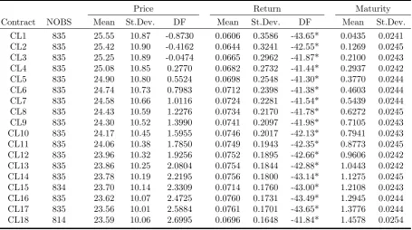
Table 1: Descriptive Summary Statistics of Crude Oil Futures

This table reports summary statistics for the crude oil futures data. The first column reports the futures Bloomberg Ticker wherein the number corresponds to the maturity in months. Prices are in US Dollars per barrel. DF stands for the Dickey-Fuller test of a unit root. * indicates significance at the 1% level.

Price Return Maturity

Contract NOBS Mean St.Dev. DF Mean St.Dev. DF Mean St.Dev. CL1 835 25.55 10.87 -0.8730 0.0606 0.3586 -43.65* 0.0435 0.0241 CL2 835 25.42 10.90 -0.4162 0.0644 0.3241 -42.55* 0.1269 0.0245 CL3 835 25.25 10.89 -0.0474 0.0665 0.2962 -41.87* 0.2100 0.0243 CL4 835 25.08 10.85 0.2770 0.0682 0.2732 -41.44* 0.2937 0.0242 CL5 835 24.90 10.80 0.5524 0.0698 0.2548 -41.30* 0.3770 0.0244 CL6 835 24.74 10.73 0.7983 0.0712 0.2398 -41.38* 0.4603 0.0244 CL7 835 24.58 10.66 1.0116 0.0724 0.2281 -41.54* 0.5439 0.0244 CL8 835 24.43 10.59 1.2276 0.0734 0.2170 -41.78* 0.6272 0.0245 CL9 835 24.30 10.52 1.3990 0.0741 0.2097 -41.98* 0.7105 0.0243 CL10 835 24.17 10.45 1.5955 0.0746 0.2017 -42.13* 0.7941 0.0243 CL11 835 24.06 10.38 1.7850 0.0749 0.1943 -42.35* 0.8773 0.0245 CL12 835 23.96 10.32 1.9256 0.0752 0.1895 -42.66* 0.9606 0.0242 CL13 835 23.86 10.25 2.0804 0.0754 0.1844 -42.88* 1.0443 0.0242 CL14 835 23.78 10.19 2.2195 0.0756 0.1800 -43.14* 1.1275 0.0245 CL15 834 23.70 10.14 2.3309 0.0714 0.1760 -43.00* 1.2108 0.0243 CL16 835 23.62 10.07 2.4725 0.0760 0.1731 -43.49* 1.2945 0.0244 CL17 835 23.56 10.01 2.5884 0.0761 0.1701 -43.65* 1.3776 0.0244 CL18 814 23.59 10.06 2.6995 0.0696 0.1648 -41.84* 1.4578 0.0254

is used for gasoline, another quarter for heating oil.3 _{Futures on these products are highly}

liquid.

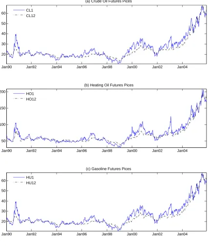
All data is obtained from Bloomberg. Figure 1 displays price paths of a short term (1

month) and a long term (12 months) future for each respective commodity. Clearly, these

prices are dependent on each other. Our data set includes also the recent strong price

increase since 2003. Descriptive summary statistics for prices and log-returns of these

contracts are reported in Tables 1, 2 and 3, respectively. For crude oil and heating oil we

consider 18 different maturities, for gasoline only 12 different contracts are available. The

relatively large standard deviations compared to former studies are caused by the sharp

price increase in the final sample period. The average maturities between the different

contracts with same maturities (in months) do deviate slightly due to different trading

3

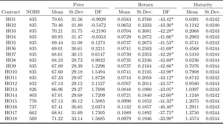
Table 2: Descriptive Summary Statistics of Heating Oil Futures

This table reports summary statistics for the heating oil futures data. The first column reports the futures Bloomberg Ticker wherein the number corresponds to the maturity in months. Prices are in US Dollar Cents per gallon. DF stands for the Dickey-Fuller test of a unit root. * indicates significance at the 1% level.

Price Return Maturity

Contract NOBS Mean St.Dev. DF Mean St.Dev. DF Mean St.Dev. HO1 835 70.65 31.56 -0.9929 0.0583 0.3760 -43.42* 0.0391 0.0242 HO2 835 70.46 31.80 -0.5472 0.0652 0.3333 -43.30* 0.1242 0.0240 HO3 835 70.21 31.75 -0.2180 0.0704 0.3081 -42.28* 0.2068 0.0243 HO4 835 69.85 31.47 -0.0353 0.0729 0.2872 -41.66* 0.2903 0.0243 HO5 835 69.44 31.08 0.1274 0.0737 0.2673 -41.53* 0.3741 0.0243 HO6 835 69.01 30.61 0.3211 0.0741 0.2503 -41.69* 0.4568 0.0244 HO7 835 68.61 30.15 0.6147 0.0739 0.2353 -42.28* 0.5410 0.0244 HO8 835 68.23 29.73 0.9022 0.0735 0.2246 -42.69* 0.6236 0.0244 HO9 835 67.89 29.39 1.2296 0.0737 0.2164 -42.86* 0.7076 0.0244 HO10 835 67.60 29.18 1.5494 0.0741 0.2105 -42.98* 0.7908 0.0244 HO11 835 67.33 29.07 1.8728 0.0744 0.2058 -43.12* 0.8742 0.0242 HO12 832 67.13 29.12 2.1527 0.0767 0.2014 -43.57* 0.9580 0.0244 HO13 826 66.96 29.27 1.7698 0.0848 0.1980 -43.05* 1.0397 0.0243 HO14 803 67.01 29.68 1.7209 0.0721 0.1840 -42.60* 1.1248 0.0242 HO15 776 67.13 30.12 1.5085 0.0990 0.1852 -41.32* 1.2075 0.0244 HO16 737 67.41 30.65 2.0374 0.1132 0.1857 -40.40* 1.2911 0.0243 HO17 662 68.81 31.69 1.7305 0.1089 0.1892 -37.75* 1.3750 0.0244 HO18 569 71.22 33.14 1.5685 0.0979 0.1946 -33.98* 1.4574 0.0244

rules regarding the last trading day.4

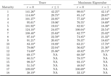
For both, the price as well as the return data, the Dickey-Fuller test of an unit root

shows clear evidence that all time series are integrated of order 1.5 _{Table 4 presents the}

results of the Johansen (1991) Trace test as well as the Maximum Eigenvalue test for

the three different futures price series with identical maturity. The results yield clear

evidence of a co-integration relationship among these commodity markets. The Trace

test of no co-integration relationship is rejected at the 1% level for all maturities. The

Maximum Eigenvalue test is significant at the 5% level for four maturities and at the 1%

4

According to to the NYMEX (www.nymex.com) the following rules apply: (i) Crude oil: Trading terminates at the close of business on the third business day prior to the 25th calendar day of the month preceding the delivery month. If the 25th calendar day of the month is a non-business day, trading shall cease on the third business day prior to the business day preceding the 25th calendar day. (ii) Heating oil and gasoline: Trading terminates at the close of business on the last business day of the month preceding the delivery month.

5

Jan90 Jan92 Jan94 Jan96 Jan98 Jan00 Jan02 Jan04 20

30 40 50 60

(a) Crude Oil Futures Pices

CL1 CL12

Jan90 Jan92 Jan94 Jan96 Jan98 Jan00 Jan02 Jan04 50

100 150 200

(b) Heating Oil Futures Pices

HO1 HO12

Jan90 Jan92 Jan94 Jan96 Jan98 Jan00 Jan02 Jan04 20

30 40 50 60

(c) Gasoline Futures Pices

HU1 HU12

Figure 1: Futures Prices

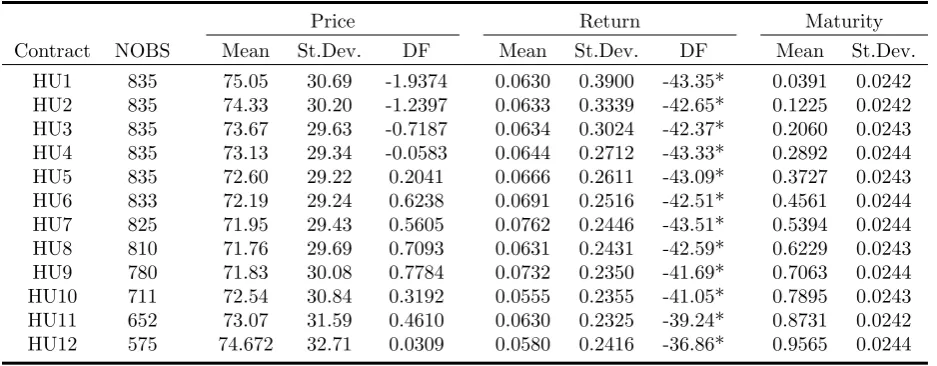
Table 3: Descriptive Summary Statistics of Gasoline Futures

This table reports summary statistics for the gasoline futures data. The first column reports the futures Bloomberg Ticker wherein the number corresponds to the maturity in months. Prices are in US Dollar Cents per gallon. DF stands for the Dickey-Fuller test of a unit root. * indicates significance at the 1% level.

Price Return Maturity

Contract NOBS Mean St.Dev. DF Mean St.Dev. DF Mean St.Dev. HU1 835 75.05 30.69 -1.9374 0.0630 0.3900 -43.35* 0.0391 0.0242 HU2 835 74.33 30.20 -1.2397 0.0633 0.3339 -42.65* 0.1225 0.0242 HU3 835 73.67 29.63 -0.7187 0.0634 0.3024 -42.37* 0.2060 0.0243 HU4 835 73.13 29.34 -0.0583 0.0644 0.2712 -43.33* 0.2892 0.0244 HU5 835 72.60 29.22 0.2041 0.0666 0.2611 -43.09* 0.3727 0.0243 HU6 833 72.19 29.24 0.6238 0.0691 0.2516 -42.51* 0.4561 0.0244 HU7 825 71.95 29.43 0.5605 0.0762 0.2446 -43.51* 0.5394 0.0244 HU8 810 71.76 29.69 0.7093 0.0631 0.2431 -42.59* 0.6229 0.0243 HU9 780 71.83 30.08 0.7784 0.0732 0.2350 -41.69* 0.7063 0.0244 HU10 711 72.54 30.84 0.3192 0.0555 0.2355 -41.05* 0.7895 0.0243 HU11 652 73.07 31.59 0.4610 0.0630 0.2325 -39.24* 0.8731 0.0242 HU12 575 74.672 32.71 0.0309 0.0580 0.2416 -36.86* 0.9565 0.0244

level for the remaining maturities. Both tests also indicate the existence of more than one

co-integrating vector at high significance levels.6

III

Integrated Commodity Model

In this section, we develop a Gaussiann-factor model for related commodity futures prices.

Our model can be viewed as an extension of Schwartz and Smith (2000)7_{. We generalize}

their model by allowing for more complex factor dependencies and we show how multiple

related commodities can be modeled simultaneously.

Uncertainty in the economy is represented by a filtered probability space (Ω,F,P), on

which an independent n-dimensional standard Brownian motion ZP

t is defined. All stochastic processes are assumed to be adapted to the filtration Ft and to be well

6

This is, of course, only true for maturities up to 12 months as there cannot be two co-integrating vectors when considering only two series.

7

Table 4: Co-Integration Analysis

This table reports the test statistics of the Johansen Trace and Maximum Eigenvalue tests. The column headlines state the null hypothesis were r is the number of co-integrating vectors. The alternative hypothesis for the trace test is a greater value of r, whereas r+ 1 is the alternative hypothesis at the maximum eigenvalue test. * indicates significance at the 1%,◦ _{at the 5% level.}

Trace Maximum Eigenvalue

Maturity r= 0 r≤1 r= 0 r= 1

1 141.26* 42.25* 99.01* 42.14*

2 114.88* 29.75* 85.14* 29.67*

3 101.27* 23.95* 77.33* 23.94*

4 95.61* 19.06◦ _76.55◦ _18.69*

5 101.92* 19.01◦ _82.91◦ _18.39*

6 124.10* 24.07* 100.04* 23.54*

7 108.40* 25.63* 82.77* 25.02*

8 97.44* 22.59* 74.85* 21.32*

9 91.21* 20.85* 70.37◦ _18.65*

10 83.10* 19.89◦ _63.21◦ _17.78*

11 78.66* 22.04* 56.62* 21.30*

12 74.69* 25.86* 48.82* 25.75*

13 69.17* NA 68.59* NA

14 80.51* NA 78.57* NA

15 99.31* NA 93.15* NA

16 51.54* NA 48.94* NA

17 109.03* NA 100.69* NA

18 38.19* NA 33.12* NA

defined satisfying the usual regularity conditions. For notational convenience conditional

expectations and variances at timetwith respect to the probability measurePof a random

vector xT are denoted by EPt[xT] and VPt [xT], respectively.

We assume that the log-spot price of commodity k can be represented by

lnSk,t =δkxt+δk0+sk(t), (1)

whereδ0

k is the constant log-price level,δk is a (1×n) vector of factor loadings, and sk(t) deterministically adjusts for seasonality effects in each commodity k. Prices are driven

by the n-dimensional vector xt of latent state variables with Gaussian diffusion

whereaP _{is a (n×1) vector andK}P _{a (n×n) positive semi-definite matrix. In the spirit}

of Schwartz and Smith (2000) we wish to decompose the price dynamics into a common

non-stationary long-term component and short-term deviations from this equilibrium.

Therefore, we assume the first state variable to follow a standard arithmetic Brownian

motion superimposed by the cross-effects of stationary Ornstein-Uhlenbeck processes.

Thus, changes in the first variable are persistent and represent fundamental changes

in the economic environment. The dependence on the weighted non-stationary factor

incorporates the empirical fact that commodity prices are not only correlated but also

co-integrated. Note that zero weights result in no co-integration. All other variables

capture deviations from the equilibrium process. As KP _{needs not be diagonal, we allow}

for interdependencies between the different factors.8 _{The model of Schwartz and Smith}

(2000) is a special case of our model with only one commodity and and a restricted matrix

KP_.

As derived in the Appendix, the state variable (xT|Ft) witht < T, is normally distributed

with mean

EP_t [xT] = ΨP(t, T)xt+ ΦP(t, T)aP (3)

and variance

V_tP[xT] = ΩP(t, T), (4)

where the matrix-valued functions ΨP_{(t, T), Φ}P_{(t, T), and Ω}P_{(t, T) are provided in}

equations (19), (20), and (21).

Following the well known interest rate literature (see e.g. Duffee (2002) and Dai and

Singleton (2002)) we allow for affine-linear market prices of risk. Consequently, the change

of measure is of the form

dZtQ=dZ P

t + (λ+ Λxt)dt

whereZtQis an orthonormal Brownian motion under the new pricing measureQequivalent

to P. λ, resp. Λ, are a (n×1), resp.(n×n) matrix of market prices of risk. Existence

8

of a risk neutral pricing measure ensures arbitrage-free prices.9 Under the risk-neutral measure the dynamics of the latent factors follow

dxt= (aQ−KQxt)dt+dWtQ. (5)

Since the factors are latent and we are interested in the model with the maximal number

of identifiable parameters we first apply the techniques presented by Dai and Singleton

(2000) and Cassasus and Collin-Dufresne (2005) to reduce equation (5) to its canonical

form. As noted by these authors we can identify in the Gaussian case as many parameters

as observing them separately. We specify the model in its canonical form underQmerely

to facilitate fast estimation. ThereforeKQ _{reduces to a (n×n) upper triangular matrix}

with elements kQi,j(i, j = 1, ..., n). The assumption of a non-stationary process in the first

state variable under the risk neutral measure implies that only the first element of aQ _is

different from zero and k₁Q,1 equals zero.

Futures Fk(t, T) with different maturities T for each commodity k are traded in the

market. Standard theory within affine frameworks implies futures prices to be equal to

the risk neutral expectation of the spot price at maturity10_{, i.e.}

lnFk(xt, t;T) = EQt [lnSk,T] +1₂VQt [lnSk,T] = δkEQt [xT] +δ0k+sk(T) + 12V

Q

t [δx,kxT] =

δkΨQ(t, T)

xt+

δkΦQ_{(t, T)a}Q₊ 1 2δkΩ

Q_{(t, T)δ}T

k +δk0+sk(T)

≡ AQ_k(t, T)xt+BQk(t, T),

(6)

where closed form solutions for the functions ΨQ_{(t, T), Φ}Q_{(t, T), and Ω}Q_{(t, T) are provided}

in the Appendix (equations (19), (20), and (21)).

Applying Ito’s lemma on lnFk(xt, t;T) one can easily recover the dynamics of Black (1976)

9

See Harrison and Pliska (1981).

10

and thus, the instantaneous volatility of returns

V_tQ[dlnFk(xt, t;T)]

dt =δkΨ

Q

(t, T)ΨQ(t, T)′

δ′

k (7)

of commodity k and the covariance between the two commoditiesk and l

CQ_t [dlnFk(xt, t;Tk);dlnFl(xt, t;Tl)]

dt =δkΨ

Q

(t, Tk)ΨQ(t, Tl)′δl′.

The spot price volatility and the long-term covariation of two commodity futures is

respectively

VQ_t [dlnSt]

dt =δkδ

′

k (8)

CQ_t [dlnFk(xt, t;Tk);dlnFl(xt, t;Tl)]

dt

T→∞

−→ δk,1δl,1. (9)

The variance structure of futures only depends on the parameters in the vectorδk at the

short end and in the long term behavior. The matrix KQ _{describes the strength of decay}

of volatility between spot prices and the long end of the term structure.

Our integrated model derived above nests many other models such as Gibson and Schwartz

(1990), Schwartz (1997), Ross (1997), and Schwartz and Smith (2000). Note that if one

wants to go along the line of Cassasus and Collin-Dufresne (2005) and incorporate a term

structure of interest rates as well, one can treat zero bonds as yet another “commodity”

k with adapted boundary conditionFk(T, T) = 1.

IV

Estimation

In this section the integrated model is implemented for crude oil, heating oil and gasoline as

a six-factor model. The choice of six latent factors is, to some extend, arbitrary. However,

as it is well known in the empirical commodity literature, two-factor models seem to do

the best job in describing the dynamics of one commodity (see e.g. Schwartz (1997)). As

Our choice is motivated for expositional reasons as well. When applying the integrated

model there will be a natural benchmark to compare our results with (see Section VI). The

entire analysis was conducted for the general case with an affine-linear market price of risk

and a restricted model, imposing Λ = 0, i.e. constant market price of risk. As the results

did not improve significantly using the unrestricted model we present the estimation for

the latter case only.11 _{Note, that this restriction implies K}P _=KQ _≡K.12

To estimate the model parameters we fit observed futures prices employing standard

Kalman filtering13_{. Thus, we are able to explore time series as well as cross-sectional}

properties of the data at the same time. It is well known that in linear and Gaussian

models, the Kalman filter is the optimal filter.

In what follows, we present the state space form of our model first in the general notation

following Harvey (1989) and afterwards using the functions derived in the previous section.

The state space transition equation can be deduced from equations (3) and (4),

xt+∆t = T xt+c+η∆t = Ψ(t, t+ ∆t)

(6×6)

xt

(6×1)

+ Φ(t, t+ ∆t)

(6×6)

aP

(6×₁₎

+ η∆t

(6×1)

(10)

for time step ∆t and η∆t serially uncorrelated, normally distributed disturbances with zero mean and constant variance

V_tP[η∆t] = Ω(t, t+ ∆t) (6×₆₎

.

The measurement equations for one commoditykat timetis given by adding measurement

errors ε to equation (6), hence

11

Allowing for affine market prices of risk adds another 36 parameters. As a consequence, already noted by Duffee (2002), the maximum likelihood function has a large number of local maxima in this framework.

12

Details on the estimation equations for the general case are available upon request.

13

yk,t

(n(k,t)×1)

= lnFk(xt, t;T) +εk,t

= Zkxt+dk+εk,t

= Ak(t, T)

(n(k,t)×₆₎

xt+Bk(t, T)

(n(k,t)×₁₎

+ εk,t

(n(k,t)×1)

(11)

whereyk,tis the vector of futures log-prices at timetof commoditykfor alln(k, t) available

maturities. The time-varying size of the matrices in (11) is due to missing observations.

All commodity prices are stacked into a vectorytof lengthn(t) = n(1, t)+n(2, t)+n(3, t).

The vector εt of serially uncorrelated, normally distributed disturbances captures the

differences between observed and theoretical prices.

Lastly, we assume the trigonometrical functional form

sk(t) = Mk

X

mk=1

γk,mkcos(2π mkt) + ¯γk,mksin(2π mkt) (12)

for the seasonality component in Bk(t, T) as proposed by Hannan et al. (1970).14 _{It is}

well known that the crude oil market does not exhibit significant seasonality and thus,

can be modelled without a seasonal component15 _{which impliesM}

1 = 0. Heating oil and

gasoline, however, do exhibit seasonal behavior. The origin of this can be directly linked

to the demand side of heating oil, which is, obviously, changing during the year. Since the

crack ratio, i.e. the ratio of heating oil and gasoline (and other minor derivatives) refined

from one barrel of crude oil cannot be changed discretionary, an increase in heating oil

production will also yield an increased production of gasoline. Consequently the price of

gasoline will decrease, as demand stays relatively stable throughout the year. As we wish

to keep our model parsimonious and there is no seasonality detectable for periods of less

than a year we choose M2 =M3 = 1.

14

This specification of the seasonality adjustment is frequently used when modelling commodity prices, for instance Sorensen (2002).

15

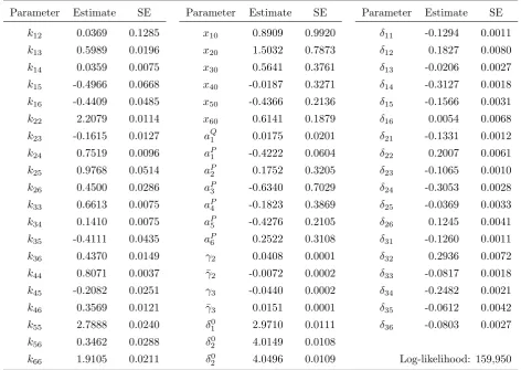
Table 5: Estimation Results

This table reports the maximum-likelihood estimates based on the Kalman filter. The sample period is 01/01/1990 through 12/31/2005 with weekly sampling frequency.

Parameter Estimate SE Parameter Estimate SE Parameter Estimate SE

k12 0.0369 0.1285 x10 0.8909 0.9920 δ11 -0.1294 0.0011

k13 0.5989 0.0196 x20 1.5032 0.7873 δ12 0.1827 0.0080

k14 0.0359 0.0075 x30 0.5641 0.3761 δ13 -0.0206 0.0027

k15 -0.4966 0.0668 x40 -0.0187 0.3271 δ14 -0.3127 0.0018

k16 -0.4409 0.0485 x50 -0.4366 0.2136 δ15 -0.1566 0.0031

k22 2.2079 0.0114 x60 0.6141 0.1879 δ16 0.0054 0.0068

k23 -0.1615 0.0127 aQ1 0.0175 0.0201 δ21 -0.1331 0.0012

k24 0.7519 0.0096 aP1 -0.4222 0.0604 δ22 0.2007 0.0061

k25 0.9768 0.0514 aP2 0.1752 0.3205 δ23 -0.1065 0.0010

k26 0.4500 0.0286 aP3 -0.6340 0.7029 δ24 -0.3053 0.0028

k33 0.6613 0.0075 aP4 -0.1823 0.3869 δ25 -0.0369 0.0033

k34 0.1410 0.0075 aP5 -0.4276 0.2105 δ26 0.1245 0.0041

k35 -0.4111 0.0435 aP6 0.2522 0.3108 δ31 -0.1260 0.0011

k36 0.4370 0.0149 γ2 0.0408 0.0001 δ32 0.2936 0.0072

k44 0.8071 0.0037 γ¯2 -0.0072 0.0002 δ33 -0.0817 0.0018

k45 -0.2082 0.0251 γ3 -0.0440 0.0002 δ34 -0.2482 0.0021

k46 0.3569 0.0121 γ¯3 0.0151 0.0001 δ35 -0.0612 0.0042

k55 2.7888 0.0240 δ

0

1 2.9710 0.0111 δ36 -0.0803 0.0027

k56 0.3462 0.0288 δ

0

2 4.0149 0.0108

k66 1.9105 0.0211 δ20 4.0496 0.0109 Log-likelihood: 159,950

V

Results

Table 5 shows the maximum likelihood parameter estimates for the data set described in

Section II. The left part reports the elements of the matrix K, which is upper diagonal.

On the right, the (3×6) matrix of factor loadings is reported. The filtered starting values

xi0, the drift vectors under the real and risk neutral measure aP and aQ, the seasonality

All elements, except for k12, of the matrix K are statistically significant. The main

diagonal elements kii can be interpreted as mean-reversion parameters as they represent

the eigenvalues of K. Their size varies from 0.66 (k33) through 2.79 (k55). Converting

these into “half-lifes” of deviations from equilibrium, we get values between 3 and 13

months, indicating different degrees of persistence of the price shocks due to the different

factors.16 _{The significance of almost all off-diagonal elements indicates their value in}

explaining the dependence structure among the three commodity markets.

The factor loadings are, except for δ16, also all significantly different from zero. The fact

that δ16 is close to zero, indicates that the sixth stochastic factor does not drive the price

of crude oil. However, δ26 as well as δ36, are non-zero, which shows that x6 captures

deviations from equilibrium on the refined product markets.

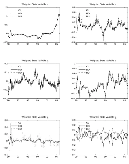
In Figure 2 the filtered state variables, weighted with their respective factor loadings are

plotted for each commodity spot price. The sum of each of the six components equals the

filtered log-spot price. Thus, we can see how each factor attributes to the three different

markets. The upper left graph displays the filtered equilibrium process. The factor loading

of the non-stationary equilibrium process, modelled by state variable x1, is non-zero for

each market. Note, that in contrast to Schwartz and Smith (2000) we do not assume

the existence of such a process ex-ante. The case of no common equilibrium factor is the

special case of our model where all or some of theδk1equal zero. Moreover, the sensitivities

towards this equilibrium process are of equal size, namely δ11 ∼= δ21 =∼ δ31 ∼= −0.13,

revealing that indeed not only a common non-stationary process can be identified, but

also that all prices react by the same degree regarding the long-term equilibrium.

The weighted state variables x2 and x4 demonstrate very similar behavior for all three

markets. Thus, they can be interpreted as shocks resulting in deviations from equilibrium

affecting all energy commodities in a similar fashion. These can be best explained by

the supply side of the market since shortages of crude oil will propagate to its refined

products markets. However, the persistence of shocks in the two state variables is different.

Whereas x2 has a half-life of 0.32 years, i.e. about 4 months, deviations due to shocks

16

from x4 take more than 10 months (half-life of 0.86 years) to halve instead. Thus, we

find two factors with different persistence levels causing deviations from equilibrium in

the energy markets considered.

The state variablex3demonstrates different behavior. Almost no contribution to the crude

oil price process, but concurrent deviations in both derivatives processes can be observed.

Thus, this state variable captures shocks mainly affecting the heating oil and gasoline

markets, but only weakly the crude oil market (δ13 is small, but statistically significant).

Analogously, the weighted factorx5 mainly captures deviation from the equilibrium in the

crude oil market, the two refined product markets are less involved. As discussed above,

δ16 is close to zero, thus the crude oil market is not affected by x6 which is also clearly

visible in the bottom right graph of Figure 2. This factor represents shocks on the refined

product markets which, in contrast to shocks due to x3, have different impacts on both

markets.

Summarizing, we are able to identify a common equilibrium process (x1), two factors

causing deviations from this equilibrium with different degrees of persistence for all

products, (x2 and x4), a factor mainly affecting the refined products in a similar way

(x3), a factor mainly capturing deviations on the crude oil market (x5), as well as one

factor only having an influence on the heating oil and gasoline markets, however, in a

distinctive fashion.

The level variables δ0

k represent the different price levels of the three commodities. These different levels are due to different trading units in the three markets as well as the costs

of the refining process, which are assumed to be constant. All three level variables are

highly significant.

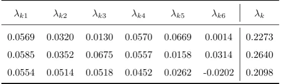
The drift parameters aQ_i and aP

i weighted with the factor loadings δij, characterize the risk premiums of the commodity spot prices with respect to the various risk factors.

More precisely, the risk premium of commodity k related to factor i can be computed

as δki(aP i −a

Q

i ) ≡ λki. Summing over all i one gets the entire risk premium for each spot commodity contract λk =

P6

Table 6: Risk premia

This table reports the risk premia for the three commodity spot prices related to the six risk factors as well as the entire risk premium of each contract.

λk1 λk2 λk3 λk4 λk5 λk6 λk

0.0569 0.0320 0.0130 0.0570 0.0669 0.0014 0.2273

0.0585 0.0352 0.0675 0.0557 0.0158 0.0314 0.2640

0.0554 0.0514 0.0518 0.0452 0.0262 -0.0202 0.2098

equilibrium factor risk premium is slightly above 0.055 for all three contracts. The overall

risk premium is 0.23 for the crude oil, 0.26 for the heating oil, and 0.21 for the gasoline

spot market.

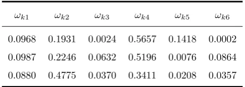
To investigate the power of the six estimated factors in explaining the variation in spot

price volatility, we calculate the ratios of factor volatilities to the overall spot price

volatility. Each factor i contributes δ2

ki ≡ ωkiδkδk′ to the entire spot price variance δkδ′k of commodity k, which can be directly seen from (7) for T → t. Table 7 displays these

ratios. The equilibrium factor explains around 10% of the variation in the three spot price

dynamics. The major part is captured by the two factors influencing all three markets,

x2 and x4. The third and the sixth factor do not contribute in explaining the variation of

crude oil prices, the fifth factor mainly drives the crude oil volatility.

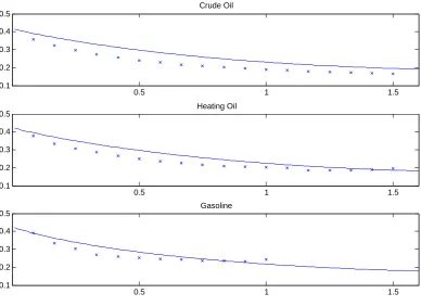
When modelling prices of financial or real assets we also wish to be able to fit the

term structure of volatilities. Equipped with the estimated parameters we are able to

compare the empirical volatilities reported in Section II with the model implied ones

using formula (7). The empirical and theoretical term structures are presented in Figure

3. The estimated term structures are slightly biased upwards, compared to the empirical

ones, but the overall shape as well as the fit at the long and short ends seem to be

satisfactory and are well in line with the Samuelson effect.17

The seasonality parameters γi and ¯γi are highly significant. To visualize the effects of

the adjustments, Figure 4 shows the trigonometric seasonality function exp(s(t)). As

17

90 93 96 99 02 05 −0.5 0 0.5 1 1.5

Weighted State Variable x₁

CL HO HU

90 93 96 99 02 05

−0.6 −0.4 −0.2 0 0.2 0.4 0.6 0.8

Weighted State Variable x₂

CL HO HU

90 93 96 99 02 05

−0.2 −0.1 0 0.1 0.2

Weighted State Variable x₃

CL HO HU

90 93 96 99 02 05

−0.4 −0.2 0 0.2 0.4 0.6 0.8 1

Weighted State Variable x₄

CL HO HU

90 93 96 99 02 05

−0.4 −0.2 0 0.2 0.4 0.6

Weighted State Variable x₅

CL HO HU

90 93 96 99 02 05

−0.4 −0.3 −0.2 −0.1 0 0.1 0.2 0.3

Weighted State Variable x₆

CL HO HU

Figure 2: Weighted State Variables

This figure shows the weighted state variables, i.e. δixi. The dotted line shows the contribution of the respective

Table 7: Explained variation

This table reports the ratios of explained variation due to the respective factor. ωki is

computed as δ

2

ki P6

i=1δ 2

ki

.

ωk1 ωk2 ωk3 ωk4 ωk5 ωk6

0.0968 0.1931 0.0024 0.5657 0.1418 0.0002

0.0987 0.2246 0.0632 0.5196 0.0076 0.0864

0.0880 0.4775 0.0370 0.3411 0.0208 0.0357

discussed in the previous section, we can observe the expected pattern of price increases

of heating oil and decrease of gasoline during the cold season and converse behavior in

the summer. The price deviations captured with this deterministic part are of the size

+/- 4% around the annual mean.

Table 8 presents summary statistics about the model fit. For each commodity and

maturity, the mean, standard deviation and maximum of the pricing errors are reported.

The crude oil futures prices are fitted best by the model. Only the one and two

months errors are slightly higher, but all middle and long-term prices are fitted very

well. Although the results are not comparable directly with the results of Schwartz and

Smith (2000), since our dataset ranges to 2005, we can observe a better fit of the model.

For instance, the one months futures standard deviation of pricing errors is 0.0226 for

our model, opposed to 0.0414 in the study of Schwartz and Smith (2000), indicating that

using information from the refined products markets can help explain the crude oil futures

prices. One could argue that the better fit is a direct result of increasing the number of

parameters. However, we do not only increase the number of stochastic factors, but also

the number of modelled commodities. Thus, comparing our results of a six factor model

for three commodity markets with a two factor model for one market seems reasonable.

The heating oil and gasoline futures prices are fitted with less precision. Again, the short

0.5 1 1.5 0.1

0.2 0.3 0.4 0.5

Crude Oil

0.5 1 1.5

0.1 0.2 0.3 0.4 0.5

Heating Oil

0.5 1 1.5

0.1 0.2 0.3 0.4 0.5

Gasoline

Figure 3: Term structure of volatilities

This figure shows the term structure of volatilities. The empirical volatilities are plot by ×, the model volatilities are given by the solid line. The maturities on the abscissa are given in years.

stable behavior.18

VI

Applications

To illustrate the economic significance of modelling multiple related commodities in an

integrated framework we consider an investment project into a refinery. In analyzing a

long-term horizon project, the differences between our approach and the ad-hoc approach

of modelling the dependencies of the considered commodities only via a correlation

structure in returns will be most noticeable.

18

Jan Apr Jul Oct Dec 0.96

0.98 1 1.02 1.04 1.06

Seasonality Adjustment

Heating Oil Gasoline

Figure 4: Seasonality adjustments

This figure shows the trigonometric seasonality adjustment function for one year.

We assume that the refinery can be described, from a financial point of view, as the

weighted sum of three cash flows. First, one has to purchase one unit of crude oil. This

is refined intoα units of heating oil and 1−αunits of gasoline which are sold in the spot

market.19 _{Thus, the present value of the refinery can be represented by the following sum}

of cash flows

P V(T) = T

X

t=1

D(0, t)[−S1,t+αS2,t+ (1−α)S3,t], (13)

where D(0, t) denotes the discount function, S1 the crude oil spot price, S2 the heating

oil spot price and S3 the gasoline spot price. To compute the distribution of P V(T) we

19

Table 8: Statistics of Pricing Errors

This table reports statistics of the pricing errors of the fitted six factor model. For each commodity and maturity mean pricing errors, standard deviation (s.d.) of pricing errors, and the maximal (max.) errors are reported. Pricing errors are computed as

et = ln(F(t, T))−ln( ˆF(t, T)) where F(t, T) denotes the observed, and Fˆ(t, T) the

fitted futures price with maturityT and timet.

Crude Oil Heating Oil Gasoline

Contract Mean S.d. Max. Mean S.d. Max. Mean S.d. Max.

Maturity Error of Error Error Error of Error Error Error of Error Error

1 -0.0034 0.0226 0.1390 0.0004 0.0281 0.1940 -0.0028 0.0366 0.1408 2 -0.0012 0.0087 0.0554 0.0003 0.0138 0.0598 -0.0027 0.0217 0.0758 3 -0.0003 0.0027 0.0149 0.0009 0.0088 0.0647 -0.0016 0.0170 0.0839 4 0.0001 0.0013 0.0067 0.0010 0.0085 0.0481 -0.0001 0.0146 0.0619 5 0.0002 0.0018 0.0084 0.0005 0.0108 0.0425 0.0007 0.0145 0.0698 6 0.0002 0.0018 0.0086 0.0001 0.0120 0.0501 0.0013 0.0160 0.0718 7 0.0001 0.0014 0.0095 -0.0001 0.0124 0.0357 0.0015 0.0172 0.0747 8 -0.0001 0.0016 0.0036 -0.0003 0.0116 0.0510 0.0018 0.0179 0.0891 9 -0.0002 0.0014 0.0104 -0.0006 0.0104 0.0396 0.0020 0.0184 0.0754 10 -0.0002 0.0016 0.0084 -0.0007 0.0101 0.0424 0.0022 0.0184 0.0739 11 -0.0002 0.0018 0.0062 -0.0011 0.0102 0.0399 0.0025 0.0191 0.0706 12 -0.0001 0.0014 0.0057 -0.0017 0.0110 0.0429 0.0040 0.0197 0.0692 13 0.0000 0.0011 0.0050 -0.0016 0.0150 0.2567

14 0.0000 0.0008 0.0030 -0.0019 0.0116 0.0414 15 0.0001 0.0011 0.0041 -0.0017 0.0125 0.0859 16 0.0002 0.0016 0.0065 -0.0015 0.0124 0.0382 17 0.0003 0.0023 0.0092 -0.0005 0.0124 0.0606 18 0.0003 0.0033 0.0197 -0.0001 0.0119 0.0653

rely on simulation as the sum of three log-normal distributed random variables is not

analytically feasible.

In our analysis we assume a risk free rate of 2%. The crack ratio α is set to 1/3, i.e.

we assume that one barrel of crude oil is refined into 0.33 barrels of heating oil and 0.67

barrels of gasoline. This ratio reflects the real ratio (0.25 and 0.5) proportionally adjusted

for neglecting the other refined products.

To put the results into perspective, we compare our integrated model with a natural

extension of Schwartz and Smith (2000) to the multiple commodity case. The latter model

5 10 15 20 25 30 −6

−4 −2 0 2 4 6x 10

4 _{Schwartz/Smith (2000) with Correlation}

years

$

Mean under P Mean under Q 10% Quantile 5% Quantile 1% Quantile

5 10 15 20 25 30

−6 −4 −2 0 2 4 6x 10

4 _{Integrated Model}

years

$

Mean under P Mean under Q 10% Quantile 5% Quantile 1% Quantile

Figure 5: Present value distribution of the refinery

This figure shows the distribution of the present value of the refinery project for the two different modelling approaches. The upper graph provides the results employing the model of Schwartz and Smith (2000) with correlated returns and the bottom graph shows the results using the integrated model. Furthermore, the present value underQis given for each model.

model for multiple commodities is to allow for non-zero correlations among the factors

driving the three different commodity price dynamics and simultaneously estimating the

model.

We evaluate the refinery from a risk management and pricing perspective, i.e. under

the real and the risk neutral measure. The mean present value as defined in (13) is

computed under Q for all T up to 30 years. Under P we simulate the entire distribution

of P V(T). The results are provided in Figure 5. The upper graph shows the present

value with respect to the maturity of the project using the extended model of Schwartz

unit per week. One can clearly observe a significant difference in the two graphs under

P, whereas the difference under Q is small. Neglecting the co-integrated behavior of the

three price processes leads to a distribution which is much wider. Considering an average

US refinery, which processes around 850,000 barrels of crude oil per week20 _{at an assumed}

profit margin of 10%, the difference of the Value-at-Risk at the 5% level after 10 years

yields approximately 400 million USD and 2.1 billion USD after 30 years.

Lastly, we show how hedging of a long-term exposure changes due to the co-movements

of prices.21 _{More precisely, we demonstrate how a single uncertain monthly cash flow}

CFT =−S1,T +αS2,T + (1−α)S3,T (14)

can be hedged efficiently. As no futures contracts for long-term horizons exist, this cannot

be done by simply going long and short in the respective contracts. However, assuming

that at least six futures contracts with distinctive underlyings or maturities are available

for continuous trading, one can build up a riskless position at each point in time t. These

hedge portfolios h are obtained by solving the following system of linear equations:

6

X

j=1

hjt

∂Fj(t, Tj)

∂xi

= ∂E Q t [CFT]

∂xi

∀i= 1, ...,6. (15)

To exemplify this hedging strategy we consider two futures on each commodity with

maturities of three and 11 months. Notice that the use of all three commodity futures is

not necessary to apply a hedging strategy within the integrated model framework. One

could also rely on only one or two of the three contracts. As the factor loadingδ16 is not

significant it will be advisable in practice to use at least one crude oil and one refined

product future. To keep things comparable we use two contracts for each commodity

since the extended model of Schwartz and Smith (2000) requires exactly this composition

of the hedging portfolio.

The hedge ratios for different maturities up to 10 years are provided in Figure 6. The

20

See the webpage of the EIA (www.eia.doe.gov).

21

5 10 −1

−0.5 0 0.5 1 1.5 2

Schwartz/Smith (2000) with Correlation

years

5 10

−1 −0.8 −0.6 −0.4 −0.2 0 0.2 0.4

0.6 Integrated Model

years

h₁ h₂ h₃ h₄ h₅ h₆

h₁ h₂ h₃ h₄ h₅ h₆

Figure 6: Hedge ratios

This figure shows the hedge positions in the six contracts considered to hedge one monthly cash flow of the refinery atT, whereT is on the abscissa. The upper graph gives these positions using the model of Schwartz and Smith (2000) incorporating correlations in returns, the lower graph provides the hedge positions implied by the integrated model.

upper graph shows the hedging demand employing the benchmark model, whereas the

lower graph shows the hedge positions in the integrated model. It is clearly visible that

both strategies differ massively. In the first case, the position in futures needed increases

up to a maturity of one year and afterwards remains significantly different from zero

between 0.7 and 1.6 contracts. On the contrary, the hedging positions in the integrated

model decrease fast, yielding a hedging demand for a five years maturity which is already

0.02.22 Thus, using the benchmark model for hedging a position in crude oil, heating oil and gasoline leads to a huge overhedge causing transaction costs to negatively affect the

project’s financial success.

VII

Summary and Conclusion

In this paper we investigate the problem of modelling multiple commodities within a

single stochastic framework. This is of high relevance for any market participant being

exposed to risks related to more than one commodity. As a concrete example we consider

a refinery, the financial success of which is highly dependent on the prices of its main

resource, crude oil and its selling products which are mainly heating oil and gasoline.

In the first step, we argue and show that the considered commodity prices are not

only correlated but also co-integrated. This fact will alter the results of any economic

evaluation, and therefore, must be considered when developing and applying a model

describing the joint stochastic price dynamics.

Applying essential-affine modelling technique we develop an integrated latent factor

model allowing for a common stochastic trend as well as any number of stationary

processes which represent deviations from the long-term equilibrium. This model captures

well known properties of commodity prices23_{, namely backwardation, mean reversion,}

declining volatilities with contract horizon, seasonality as well as the co-integrated

behavior described above. Furthermore, it nests many well known models such as Gibson

and Schwartz (1990), Schwartz (1997), Schwartz and Smith (2000), and Cassasus and

Collin-Dufresne (2005).24

22

The fact of decreasing hedging demand with increasing maturity is an implication of the equal sensitivities towards the common equilibrium process. Considering exemplary two commodities, the variance of a futures contract which exchanges commodity k forl at timeT, −Sk,T +Sl,T, will have a

variance of approximately (δ2

k,1−2δk,1δl,1+δ 2

l,1)∼= 0,ifδk,1∼=δl,1. 23

See e.g. Routledge et al. (2000).

24

Using NYMEX futures data, a six factor model for crude oil, heating oil and gasoline

is estimated using standard Kalman filtering and maximum likelihood. We find that

the core features of our model are highly significant. We are not only able to identify

a non-stationary common long-term component driving all commodity prices but also

find that all commodities exhibit the same factor loading. Two of the stationary factors

impact the markets in a common fashion, however with different levels of persistence. In

contrast, the other three components influence the three commodities in a distinctive way.

To emphasize the economic significance of our results we apply the integrated model in

the context of a refinery. From the viewpoint of risk management, the dispersion of the

present value distribution decreases severely when compared to an approach neglecting

the co-movements of commodity prices. Finally, we show when hedging a single cash flow

with short-term futures contracts, the optimal hedging changes considerably for short,

and even more for long horizons. For the latter case, the hedging demand decreases

A

Appendix

Consider the dynamics

dxt = (aM −KMxt)dt+dZtM

under anyP-equivalent measure M, where ZM

t is a standard Brownian motion under M,

aM _{is a constant vector andK}

M is a positive semi-definite constant matrix. Decomposing the matrix KM _{≡ U V U}−1 _{where V is the diagonal matrix of distinctive eigenvalues}

{vi ≥0} of KM and U the matrix of associated eigenvectors. Defining the functions

ψ(v;t, T) = exp(−v(T −t))−→v→0 1 (16)

and

φ(v;t, T) =

Z T

t

ψ(v;s, T)ds = (1−exp(−v(T −t))

v

v→0

−→(T −t) (17)

and the matrix

Lψ(KM;t, T) =

       

ψ(v1;t, T) 0 · · · 0

0 ψ(v2;t, T) · · · 0

... ... . .. ... 0 0 0 ψ(vn;t, T)

        (18)

and Lφ analogously, where the function ψ is replaced by φ. Integrating the matrix Lψ

from t to T results in the matrix Lφ. The matrix ULψ(KM;t, T)U−1 can be seen as matrix-valued equivalent to the function exp(−k(T −t)).

First, applying Ito’s lemma to the the function ULψ(KM_{;t, T)U}−1_{xt, with}

∂(UL_ψ(KM_;t,T)U−1₎

∂t =ULψ(K

M_{;t, T)U}−1_{K, results in}

d(ULψ(KM_{;s, T)U}−₁

xt) = ULψ(KM_{;s, T)U}−₁

aM_dt+ULψ(KM_{;t, T)U}−₁

then integration of the LHS results in

Z T

t

d(ULψ(KM;s, T)U−1_{xs) = ULψ(K}M

;T, T)U−1_x

T −ULψ(KM;t, T)U

−1_x

t = xT −ULψ(KM;t, T)U−1xt.

Rearranging yields

xT = ULψ(KM;t, T)U

−₁

xt+

Z T

t

ULψ(KM;s, T)U−1aMdt

+

Z T

t

ULψ(KM;s, T)U

−₁

dZsM

as the solution.

Thus, (xT|Ft) is Gaussian and the conditional expected value can be calculated as

EM_t [xT] = ULψ(KM;t, T)U

−₁

xt+

Z T

t

ULψ(KM;s, T)U

−₁

aMds

= ULψ(KM;t, T)U

−₁

xt+U

Z T

t

Lψ(KM;s, T)ds

U−1aM

= ΨM(t, T)xt+ ΦM(t, T)aM

with

ΨM(t, T) = ULψ(KM;t, T)U−1 (19)

as well as the conditional variance as

VM_t [xT] = EMt [

Z T

t

(ULψ(KM;s, T)U−1_dZM

t )(ULψ(KM;s, T)U

−1_dZM t )

′

]

=

Z T

t

ULψ(KM;s, T)(U

−1_U′−1

)L′

ψ(KM;s, T)U′

ds

= U Z T

t

Lψ(KM;s, T)HL

′

ψ(KM;s, T)ds U

′

= UH(KM;t, T)U′

= ΩM(t, T) (21)

where H ≡U−1_U′−1

and the matrix H can be easily derived by considering one element

Hij of the matrix H

Z T

t

ψ(vi;s, T)Hijψ(vj;s, T)ds =

Z T

t

Hijψ(vi+vj;s, T)ds

= Hijφ(vi+vj;s, T)

References

F. Black. The pricing of commodity contracts. Journal of Financial Ecomomics, 3: 167–179, 1976.

J. Cassasus and P. Collin-Dufresne. Stochastic convenience yield implied from commodity futures and interest rates. Journal of Finance, 60(5):2283–2331, 2005.

Q. Dai and K.J. Singleton. Specification analysis of affine term structure models. Journal of Finance, 55(5):1943–1978, 2000.

Q. Dai and K.J. Singleton. Expectation puzzles, time-varying risk premia, and affine models of the term structure. Journal of Financial Economics, 63:415–441, 2002.

G. R. Duffee. Term premia and interest rate forecasts in affine models.Journal of Finance, 57(1):405–443, 2002.

R. Gibson and E. S. Schwartz. Stochastic convenience yield and the pricing of oil contingent claims. Journal of Finance, 45:959–976, 1990.

O. Gjolberg and T. Johnson. Risk management in the oil industry: can information on long-run equilibrium prices be utilized? Energy Economics, 21:517–527, 1999.

E. J. Hannan, R. D. Terrell, and N. E. Tuckwell. The seasonal adjustment of economic time series. International Economic Review, 11(1):24–52, 1970.

J. M. Harrison and S. R. Pliska. Martingales and stochastic integrals in the theory of continuous trading. Stochastic Process. Appl., 11(3):215–260, 1981.

A. C. Harvey.Forecasting, structural time series models and the Kalman filter. Cambridge University Press, 1989.

S. Johansen. Estimation and hypothesis testing of cointegration vectors in Gaussian vector autoregressive models. Econometrica, 59(6):1551–1580, 1991.

O. Korn. Drift matters: An analysis of commodity derivatives. Journal of Futures Markets, 25(3):211–241, 2005.

M. Manoliu and S. Tompaidis. Energy futures prices: term structure models with Kalman filter estimation. Applied Mathematical Finance, 9:21–43, 2002.

R.S. Pindyck and J.J. Rotemberg. The excess co-movement of commodity prices. The

Economic Journal, 100:1173–1189, 1990.

S. A. Ross. Hedging long run commitments: Exercises in incomplete market pricing.

Banca Monte Economic Notes, 26:99–132, 1997.

B R. Routledge, D J. Seppi, and C S. Spatt. Equilibrium forward curves for commodities.

Journal of Finance, 55(3):1297–1338, 2000.

P. Samuelson. Proof that properly anticipated prices fluctuate randomly. Industrial

Management Review, 6:41–49, 1965.

E. S. Schwartz. The stochastic behavior of commodity prices: Implication for valuation and hedging. Journal of Finance, 52(3):923–973, 1997.

E. S. Schwartz and J. E. Smith. Short-term variations and long-term dynamics in commodity prices. Management Science, 46(7):893–911, 2000.