Volume 2007, Article ID 57956,7pages doi:10.1155/2007/57956
Research Article
Product Bessel Distributions of the First and Second Kinds
Saralees Nadarajah
Received 15 August 2005; Accepted 11 February 2007
Recommended by Andrew Rosalsky
A new Bessel function distribution is introduced by taking the product of a Bessel func-tion pdf of the first kind and a Bessel funcfunc-tion pdf of the second kind. Various particular cases and expressions for moments are derived.
Copyright © 2007 Saralees Nadarajah. This is an open access article distributed under the Creative Commons Attribution License, which permits unrestricted use, distribution, and reproduction in any medium, provided the original work is properly cited.
1. Introduction
Univariate Bessel function distributions have been used to model signal output processed by a radar receiver under various sets of conditions (see, e.g., McNolty [1]). There are two kinds of univariate Bessel function distributions. Bessel function distribution of the first kind has the pdf given by
f(x)= 1−c2 m+1/2
xm √
π2mbm+1Γ(m+ 1/2)exp
−cx
b
Im
x b
(1.1)
forx >0,b >0,c >1 andm >1, where
Im(x)= x m √
π2mΓ(m+ 1/2)
1
−1
1−t2m−1/2exp(±xt)dt (1.2)
is the modified Bessel function of the first kind. Bessel function distribution of the second kind has the pdf given by
f(x)= 1−c2 m+1/2
|x|m √
π2mbm+1Γ(m+ 1/2)exp
−cx
b
Km
for−∞< x <∞,b >0,|c|<1, andm >1, where
Km(x)= √
πxm
2mΓ(m+ 1/2)
∞
1
t2−1m−1/2exp(−xt)dt (1.4)
is the modified Bessel function of the second kind. In thispaper, we introduce a new Bessel function distribution with its pdf taken to be the product of two densities of the form (1.1) and (1.3), that is,
f(x)=Cxm+nI m
x b
Kn
x β
(1.5)
forx >0, 0< β < b,m >1, andn >1, whereCdenotes the normalizing constant. Appli-cation of [2, equation (2.16.28.1)] by Prudnikov et al. shows that one can determineC
as
1
C=
2m+n−1β2m+n+1
bmΓ(m+ 1) Γ
m+n+1 2
Γm+1 2
2F1
m+n+1 2,m+
1 2;m+ 1;
β2
b2
, (1.6)
where2F1is the Gauss hypergeometric function defined by
2F1(a,b;c;x)=
∞
k=0
(a)k(b)k
(c)k
xk
k!, (1.7)
where (f)k=f(f+ 1)···(f+k−1) denotes the ascending factorial. Using special
prop-erties of the Gauss hypergeometric function, one can obtain simpler expressions for (1.6). For instance, ifm=n, then (1.6) can be reduced to
1
C=π−
1/222m−1(bβ)2m+1/2b2−β2−mΓ2m+ 1
2
×exp(miπ)Qmm−1/2
b2+β2
2bβ
,
(1.8)
whereQνμ(·) is the Legendre function defined by
Qμν(x)= √
πexp(iμπ)Γ(μ+ν+ 1) 2ν+1Γ(ν+ 3/2) x
−μ−ν−1x2−1μ/2 2F1
μ+ν+ 1
2 ,
μ+ν 2 ;ν+
3 2;
1
x2
.
(1.9)
2. Particular cases
Whenmandntake half-integer values, one can reduce (1.5) to elementary forms. Note that
I3/2(x)= 2
π
xcosh(x)−sinh(x)
x3/2 ,
I5/2(x)= 2
π
x2+ 3sinh(x)−3xcosh(x)
x5/2 ,
I7/2(x)= 2
π
xx2+ 15cosh(x)−32x2+ 5sinh(x)
x7/2 ,
I9/2(x)= 2
π
x4+ 45x2+ 105sinh(x)−5x2x2+ 21cosh(x)
x9/2
(2.1)
and, more generally, ifν−1/2≥1 is an integer, then
Iν(x)=√2√xπexp
πi
2 1
2−ν × sinh πx 2 1 2−ν
−x
×
[(2|ν|−1)/4]
k=0
|ν|+ 2k−1/2! (2k)!|ν| −2k−1/2!(2x)2k
+ cosh
πx
2 1
2−ν
−x
[(2|ν|−3)/4]
k=0
|ν|+ 2k+ 1/2!(2x)−2k−1
(2k+ 1)!|ν| −2k−3/2!
.
(2.2)
Furthermore, note that
K3/2(x)=
π
2
exp(−x)(x+ 1)
x3/2 ,
K5/2(x)=
π
2
exp(−x)x2+ 3x+ 3
x5/2 ,
K7/2(x)=
π
2
exp(−x)x3+ 6x2+ 15x+ 15
x7/2 ,
K9/2(x)=
π
2
exp(−x)x4+ 10x3+ 45x2+ 105x+ 105
x9/2
(2.3)
and, more generally, ifν−1/2≥1 is an integer, then
Iν(x)=√πexp(−x)√2x [|ν|−1/2]
j=0
j+|ν| −1/2!(2x)−j
j!|ν| −j−1/2! . (2.4)
Thus, several particular forms of (1.5) can be obtained for half-integer values ofmandn. For example, ifm=3/2 andn=3/2, then (1.5) reduces to
f(x)=C(bβ)3/2 x bcosh x b −sinh x b exp −x β x β+ 1
0 1 2 3 4 5 x
0 0.1 0.2 0.3
(a)
0 1 2 3 4 5
x 0
0.1 0.2 0.3
(b)
0 1 2 3 4 5
x 0
0.1 0.2 0.3
(c)
0 1 2 3 4 5
x 0
0.1 0.2 0.3
(d)
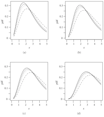
Figure 2.1. Plots of the pdf (1.5) forb=1,β=1/2, and (a)m=1.1; (b)m=1.3; (c)m=1.5; and, (d)m=2. The four curves in each plot from the left to the right correspond ton=1.1, 1.3, 1.5, 2.
Ifm=3/2 andn=5/2, then (1.5) reduces to
f(x)=Cb3/2β5/2
x bcosh
x b
−sinh
x b
exp
−x
β
x2
β2+
3x β + 3
. (2.6)
3. Moments
IfXis a random variable with pdf (1.5), then itskth moment can be expressed as
EXk=C
∞
0 x k+m+nI
m x b Kn x β dx. (3.1)
Application of [2, equation (2.16.28.1)] by Prudnikov et al. shows that (3.1) can be cal-culated as
EXk=C2k+m+n−1βk+2m+n+1
bmΓ(m+ 1) Γ
m+n+k+ 1 2
Γm+k+ 1 2
×2F1
m+n+k+ 1 2 ,m+
k+ 1 2 ;m+ 1;
β2
b2
.
(3.2)
Using special properties of the Gauss hypergeometric function, one can derive several simpler forms of (3.2) as discussed in the following. Ifm=n, then (3.2) reduces to
EXk=Cπ−1/22k+2m−1(bβ)k+2m+1/2b2−β2−(k+2m)/2Γ
k+ 2m+ 1 2
×exp
(k+ 2m)iπ
2
Q(mk−+21m/2)/2
b2+β2
2bβ
.
(3.3)
Ifk≥1 is odd, then (3.2) can be reduced to the following elementary form:
EXk=C2k+m+n−1bk+m+2n+1βk+2m+n+1
b2−β2m+n+(k+1)/2Γ(m+ 1) Γ
m+n+k+ 1 2
Γm+k+ 1 2
×2F1
m+n+k+ 1 2 ,
1−k
2 ;m+ 1;
β2
β2−b2
=C2k+m+n−1bk+m+2n+1βk+2m+n+1
b2−β2m+n+(k+1)/2Γ(m+ 1) Γ
m+n+k+ 1 2
Γm+k+ 1 2
× (k−1)/2
j=0
m+n+ (k+ 1)/2j(1−k)/2j (m+ 1)j
β2
β2−b2
j
.
(3.4)
Whenk is even, one can reduce (3.2) to simpler forms whenmandn take integer or half-integer values. If either bothmandnare half-integers ormis an integer andnis a half-integer ormis a half-integer andnis an integer, then (3.2) can be reduced to an elementary form. On the other hand, if bothmandnare integers, then one can express (3.2) in terms of the complete elliptical integral of the first kind and the complete elliptical integral of the second kind defined by
EllipticK(a)=
1
0
dx
√
1−x2√1−a2x2dx,
EllipticE(a)=
1
0 √
1−a2x2 √
1−x2 dx,
respectively. For instance, ifm=3/2 andn=3/2, then the first four even order moments are
EX2=8Cβ15/2−35−14x+x
2
b3/2(−1 +x)5 ,
EX4=144Cβ19/2−105−189x−27x2+x3
b3/2(−1 +x)7 ,
EX6=5760Cβ23/2−231−924x−594x2−44x3+x4
b3/2(−1 +x)9 ,
EX8=403200Cβ27/2−429−3003x−4290x2−1430x3−65x4+x5
b−3/2(−1 +x)−11 ,
(3.6)
wherex=β2/b2and the normalizing constantC=2β11/2(−5 +x)/{b3/2(−1 +x)3}. Ifm=
2 andn=2, then the first four even order moments are
EX2=15Cβ9−23 EllipticK(√x)x−87 EllipticK(√x)x2+ 107 EllipticK(√x)x3
+ EllipticK(√x)x4+ 2 EllipticK(√x) + 22 EllipticE(√x)x
+ 216 EllipticE(√x)x2+ 22 EllipticE(√x)x3−2 EllipticE(√x)x4 −2 EllipticE(√x)/x2b2(−1 +x)6,
EX4=315Cβ11−39 EllipticK(√x)x−536 EllipticK(√x)x2+ 158 EllipticK(√x)x3
+ 414 EllipticK(√x)x4+ EllipticK(√x)x5+ 2 EllipticK(√x)
+ 38 EllipticE(√x)x+ 988 EllipticE(√x)x2+ 988 EllipticE(√x)x3
+ 38 EllipticE(√x)x4−2 EllipticE(√x)x5 −2 EllipticE(√x)/x2b2(−1 +x)8,
EX6=2835Cβ13−295 EllipticK(√x)x−8771 EllipticK(√x)x2−8886 EllipticK(√x)x3
+ 12452 EllipticK(√x)x4+ 5485 EllipticK(√x)x5+ 5 EllipticK(√x)x6
+ 10 EllipticK(√x) + 290 EllipticE(√x)x+ 14546 EllipticE(√x)x2
+ 35884 EllipticE(√x)x3+ 290 EllipticE(√x)x5
+ 14546 EllipticE(√x)x4−10 EllipticE(√x)x6 −10 EllipticE(√x)/(−1 +x)10x2b2,
EX8=155925Cβ1514 EllipticK(√x)−581 EllipticK(√x)x−30336 EllipticK(√x)x2 −86111 EllipticK(√x)x3+ 19958 EllipticK(√x)x4
+ 80445 EllipticK(√x)x5+ 16604 EllipticK(√x)x6
+ 7 EllipticK(√x)x7−14 EllipticE(√x) + 574 EllipticE(√x)x
+ 47514 EllipticE(√x)x2+ 214070 EllipticE(√x)x3
+ 47514 EllipticE(√x)x5+ 214070 EllipticE(√x)x4
wherex=β2/b2and the normalizing constantCsatisfies
1
C=3β
7−11 EllipticK(√
x)x+ 8 EllipticK(√x)x2+ EllipticK(√x)x3+ 2 EllipticK(√x)
+ 10 EllipticE(√x)x+ 10 EllipticE(√x)x2−2 EllipticE(√x)x3 −2 EllipticE(√x)/x2b2(−1 +x)4.
(3.8)
References
[1] F. McNolty, “Applications of Bessel function distributions,” Sankhy¯a, vol. 29, pp. 235–248, 1967. [2] A. P. Prudnikov, Y. A. Brychkov, and O. I. Marichev, Integrals and Series. Vol. 2, Gordon & Breach
Science Publishers, New York, NY, USA, 1986.