M atching, E ducation E xternalities and
th e Location o f Econom ic A ctiv ity
Thesis submitted for the degree of
Doctor of Philosophy (Ph.D.) by Pablo Burriel Llombart
registered at the London School of Economics
UMI Number: U61BB39
All rights reserved
INFORMATION TO ALL USERS
The quality of this reproduction is dependent upon the quality of the copy submitted.
In the unlikely event that the author did not send a complete manuscript and there are missing pages, these will be noted. Also, if material had to be removed,
a note will indicate the deletion.
Dissertation Publishing
UMI U613339
Published by ProQuest LLC 2014. Copyright in the Dissertation held by the Author. Microform Edition © ProQuest LLC.
All rights reserved. This work is protected against unauthorized copying under Title 17, United States Code.
ProQuest LLC
789 East Eisenhower Parkway P.O. Box 1346
d
QNV ^
A ck n ow led gem en ts
I am most grateful to my supervisor Professor Christopher Pissarides for his ad
vice and guidance throughout my PhD. I am also thankful to him for providing
me with the opportunity to undertake this thesis in the excellent environment of the Centre for Economic Performance at the London School of Economics.
While working on this thesis I have benefited from helpful comments and sug
gestions from a great number of friends and colleagues. I would like to thank
Dr. Ricardo Lagos, Dr. Frangois Ortalo-Magne and Professor Steve Nickell
for providing invaluable comments and suggestions on the theoretical chapters
and Dr. Barbara Petrongolo, Dr. Steve Pischke, Dr. Hillary Steedman and Dr. Jonathan Wadsworth for their very helpful comments on the empirical chap
ters of this thesis. I would like to express my gratitude to Glenda Quintini
for providing me with her dataset on regional wages from the New Earnings
Survey and to Jonathan Wadsworth, Richard Dickens and Susan Harkness for allowing me to use their Stata codes to work with the Labour Force Survey.
I would also like to thank Richard Barwell, Merxe Tudela, Maria Guadalupe
and Paloma Lopez-Garcia for very interesting and helpful discussions on econo metric and theoretic issues related to my thesis. Participants at the Labour
Markets Workshop, Macro-International Workshop and Macro Workgroup at
the Centre for Economic Performance provided very useful comments.
I am indebted to Martin Stewart and Richard Barwell for proof-reading my
English and thereby enhancing the quality of this thesis.
I would like to acknowledge financial support from Banco de Espana.
I would also like to thank Javier Andres for pushing me to leave the cosy en
vironment of Universidad de Valencia.
A b stra ct
In this thesis we demonstrate how important the existence of a pool of qual
ified workers within the local labour market is for the process of job creation
and the location of economic activity.
In chapter 1 the basic theoretical model is developed. Using a matching model it is shown th at Job Creation will be higher if firms have a larger pool of qual
ified workers from which to fill their vacancies, since their expected profits per
vacancy opened will be greater. At the same time, individuals have a higher
incentive to invest in education if job creation is higher. The interaction be
tween these two forces generates a pecuniary externality in the labour market.
In chapter 2, we extend the theoretical model by considering two regions and
the possibility of migration. In equilibrium, areas where the pool of qualified
workers is larger attract more jobs and skilled workers. Job Creation will be
higher in such areas since firms located there are able to find a more qualified worker with greater ease. At the same time, given the sunk cost of moving,
only the most skilled workers will find migration to these areas worthwhile.
The interaction between these two forces generates a pecuniary externality
th at encourages concentration of economic activity in areas with a larger pool of qualified workers.
In chapter 3 we estimate the effect of the pecuniary education externality on
the process of matching in the UK regional labour market in the 1990s. We
find a significant effect of the average level of education in a region on the
conditional probability of finding a job in that region using a duration model.
This effect is positive for skilled occupations and negative for unskilled ones.
Finally, in Chapter 4 we estimate the effect of the education externality on
the individual decision to stay-on in education. We find th at the share of
the region’s working age population with degree has a positive and significant
effect on the education decisions of sixteen and eighteen year-olds, while the
C on ten ts
1 Job creation and increasing returns H
1.1 In tro d u ctio n ...H
1.2 Description of the E c o n o m y ... 14
1.3 Labor Market E q u ilib riu m ...17
1.4 Equilibrium of the E co n o m y ...23
1.5 Social Planner’s S o lu tio n ... 29
1.6 Physical C a p ita l...30
1.7 Different Unemployment Rates ...33
1.8 C o n clu sio n s...35
2 Location and m atching extern alities 37 2.1 In tro d u ctio n ... 37
2.2 Description of the E c o n o m y ...40
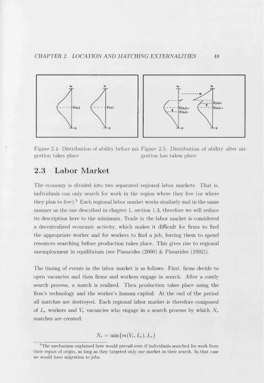
2.3 Labor M a r k e t...48
2.4 Regional E q u ilib riu m ... 30
2.5 Equilibrium of the E co n o m y ... 34
2.6 Welfare a n aly sis...30
2.7 C o n clu sio n s... 32
3 E ducation externalities in m atching 33 3.1 In tro d u ctio n ... 33
3.2 Theoretical m o d e l...37
3.3 The d a t a ... 39
3.4 Econometric specification... 32
3.5 R esu lts...36
3.6 Vacancy Creation and Education Externalities... 103
3.7 C o n clu sio n s... HO
4 Education externalities in education 112
4.1 In tro d u ctio n ... 112
4.2 Theoretical m o d e l... 118
4.3 The d a t a ... 121
4.4 R esu lts... 133
4.5 Robustness of R esu lts... 143
4.6 Participation rate in education...146
4.7 C o n clu sio n s... 147
A A ppendix for C hapter 1 148 A.l Level of education in the Social Planner’s so lu tio n ...148
A.2 Additional Figures of chapter 1 ...149
B A ppen dix for Chapter 2 150 B.l Derivatives of equilibrium eq u atio n s... 150
B.2 Derivatives of equilibrium equations with respect to the param eters of the e c o n o m y ... 151
C A ppen dix for Chapter 3 153 C .l Definition of Education Variable... 153
C.2 Definition of the variables used in the estimation...154
C.3 Classification of regions... 155
C.4 Econometric Method to correct for stock sampling bias...156
C.5 Additional tables &; figures of Chapter 3... 157
D A ppen dix for Chapter 4 174 D.l Definition of the variables used in the estimation...174
List o f Tables
2.1 Comparative s ta tic s ...' ... 57
3.1 Categories of Education and Occupation v a ria b les...72
3.2 Sample means of individual characteristics by occupation group 73
3.3 Average Education by 4 Occupation G r o u p s ...75
3.4 Average Education by Region and Occupation Group, top 5 & bottom 5 r e g io n s ... 77
3.5 Average Annual Growth Rate of Average Education by Occu
pation, top 5 & bottom 5 r e g io n s ...78
3.6 Maximum likelihood estimates of re-employment probabilities
by occupation g r o u p ... 87 3.7 Average % change in baseline hazard of the representative indi
vidual ... 91
3.8 Maximum likelihood estimates of re-employment probabilities by sex and occupation g ro u p ... 92
3.9 Maximum likelihood estimates of re-employment probabilities
by age group and occupation g r o u p ... 92
3.10 Maximum likelihood estimates of re-employment probabilities
by occupation group using all the durations in the sample, con
trolling for entrance to sample...94
3.11 Maximum likelihood estimates of re-employment probabilities
by occupation group dropping industrial s h a r e ...95
3.12 Maximum likelihood estimates of re-employment probabilities
by occupation group, more disaggregated... 100
3.13 Maximum likelihood estimates of re-employment probabilities
by occupation group allowing for Gamma distributed individual
unobserved heterogeneity... 101
3.14 Maximum likelihood estimates of re-employment probabilities by occupation group dropping top & bottom region in education 104
3.15 Maximum likelihood estimates of transitions to inactivity . . . . 107
3.16 Fixed Effects estimation of the Vacancy rate by quarter, region and o c c u p a tio n ...109
4.1 Sample means of variables by s ta y in g -o n ... 126
4.2 Education’s share of UK’s working age p o p u la tio n ... 128
4.3 Education’s share of working age population by 5 top regions . . 130 4.4 Education’s share of working age population by 5 bottom regions 130 4.5 Education decisions in the U K ... 131
4.6 Probit estimation of the individual’s probability of staying-on in e d u c a tio n ... 134
4.7 Change in expected probability of representative individual af ter a change in the workforce’s share by education (percentage points) ... 137
4.8 Change in expected probability of representative individual af ter a change in the unemployment rate by education (percentage points) ... 139
4.9 Change in expected probability of representative individual af ter a change in permanent earnings by education (percentage points) ... 141
C .l Education V a ria b le ... 153
C.2 Classification of regions... 155
C.3 Average Education by Region and Occupation G r o u p ... 157
C.4 Average Annual Growth Rate of Average Education by Occu pation ... 158
C.5 Maximum likelihood estimates of re-employment probabilities by sex and occupation group. Individual c o n t r o l s ...161
C.6 Maximum likelihood estimates of re-employment probabilities by age group and occupation group. Individual controls... 162
C.8 Maximum likelihood estimates of re-employment probabilities
by occupation group dropping industrial share. Individual con
trols... 165
C.9 Maximum likelihood estimates of re-employment probabilities by occupation group, more disaggregated. Individual controls. . 167
C.10 Maximum likelihood estimates of re-employment probabilities by occupation group controlling for Gamma distributed unob served heterogeneity. Individual controls... 168
C .ll Maximum likelihood estimates of re-employment probabilities by occupation group dropping top & bottom region in educa tion. Individual controls... 170
C.12 Maximum likelihood estimates of transitions to inactivity. In dividual controls ...172
D .l Education attainment of stayers and leavers by a g e ...176
D.2 Region’s ranking by education. Top 5 regions ... 177
D.3 Region’s ranking by education. Bottom 5 regions ...177
D.4 Probit estimation of the individual’s probability of participating in e d u c a tio n ... 178
D.5 Probit estimation of the individual’s probability of staying on &; participating in education not controlling for ability ... 180
D.6 Probit estimation of the individual’s probability of staying on & participating in education dropping top & bottom regions . . 182
List o f F igures
1.1 Labour Market Equilibrium case 1: 9max < | ... 21
1.2 Labour Market Equilibrium case 2: 9max > | ...21
1.3 Rise in E[ha]. Case 2: 9max > J ...23
1.4 Equilibrium of the economy. Case 1: unemployment equilibrium 24 1.5 Equilibrium of the economy. Case 2: full em ploym ent... 24
1.6 Equilibrium of the economy. Case 3: no economic activity . . . 25
1.7 Case 3: Equilibrium of the economy with compulsory education 28 2.1 Average regional education duration vs labour market tightness 39 2.2 Average regional education duration vs unemployment duration 39 2.3 Evolution of regional average ability as migration increases . . . 47
2.4 Distribution of ability before migration takes place ... 48
2.5 Distribution of ability after migration has taken p la c e ... 48
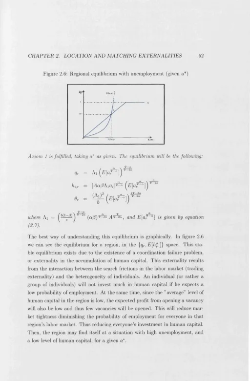
2.6 Regional equilibrium with unemployment (given a * ) ... 52
2.7 Effect of an increase in migration (reduction in a*) in region j . 53 2.8 Effect of an increase in migration (reduction in a*) in region g . 53 2.9 Equilibrium of the e c o n o m y ...55
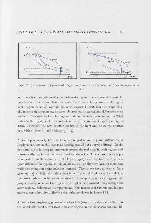
2.10 Equilibrium of the economy comparing regional labour markets 56 2.11 Increase in the cost of migration ( m ) ... 58
2.12 Increase in 6, or decrease in L or c... 58
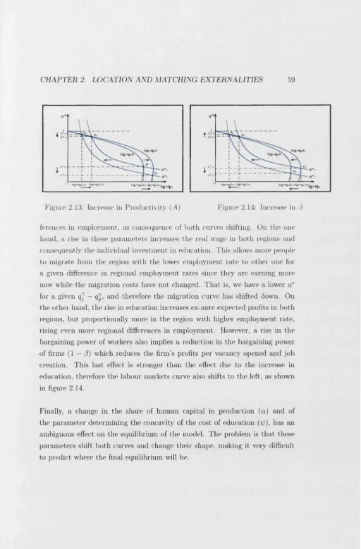
2.13 Increase in Productivity ( A ) ...59
2.14 Increase in /? ...59
3.1 Average education by occupation ( G B ) ... 76
3.2 Average education vs average growth of education by occupa tion (line with crosses excludes 3 top & bottom regions) . . . . 76
3.3 Survival by 4 occupations ...79
3.4 Survival of top Sz bottom r e g i o n s ... 79
10
3.5 Survival in state of unemployment by occupation for top & bot
tom r e g io n s ...79
3.6 Market tightness by o c c u p a tio n ...81
3.7 Average education vs labour market tightness by occupation (line with crosses excludes 3 top & bottom re g io n s ) ... 81
3.8 Baseline hazard all individuals ...90
3.9 Baseline hazard by occupation g r o u p ... 90
4.1 Staying-on in education r a t e ... 123
4.2 Participation in education r a t e ... 123
4.3 share with degree vs staying-on rate at 16 ... 132
4.4 share with degree vs staying-on rate at 1 7 ... 132
4.5 share with degree vs staying-on rate at 18 ... 132
4.6 share with degree vs participation rate at 1 7 ... 132
4.7 share with degree vs participation rate at 1 8 ... 132
A .l Equilibrium of the economy. Case 2a: full employment equilibrium 149 C .l Unemployment duration by o c c u p a tio n ... 159
C.2 Market tightness by o c c u p a tio n ...159
C.3 Average education vs unemployment duration by occupation(line with crosses excludes 3 top & bottom re g io n s )... 159
C.4 Baseline hazard by s e x ... 160
C hapter 1
Job creation and increasing
returns to hum an cap ital
1.1
In tr o d u ctio n
In this chapter we show that the interaction between ex-ante investment de
cisions of heterogeneous individuals and firms in a labor market with search
frictions generates a positive externality on the accumulation of human capital and the possibility of multiple equilibria. When individuals have to invest in
education prior to entering the labor market and firms have to decide to open
a vacancy before meeting a worker, in a labor market characterized by search frictions, there will exist a positive spill-over from each individual’s investment
in human capital to the rest of the society.
In general, individuals make their education decisions when young, well before
entering the labor market. This decisions will thus be based on the expected
probability to find a job and earn a wage. On the other hand, firms nor
mally have to decide whether to incur in the cost of opening a vacancy or not,
before knowing which worker they will be matched with. This means that
they will base their decision on the expected profits from opening a vacancy,
which will depend on the expected average of human capital among individu
als. Therefore any exogenous change in the level of education of some workers
will increase the expected profits per vacancy, augmenting job creation and
the employment rate. This will improve every individual’s expectations about
the labor market and in turn will give incentives to everyone to increase his
investment in human capital. At an aggregate level, the existence of increasing
CHAPTER 1. JOB CREATION AND INCREASING RETU RN S 12
returns might generate different equilibria dependent on the underlying param
eters. Some economies might get stuck at a low employment, low aggregate
level of human capital equilibrium, while others will enjoy full employment and
high skill level, depending on the underlying characteristics of each economy.
The interesting feature of this externality is that it does not depend on the existence of increasing returns to scale neither in the production function, nor
in the matching function. It is only due to the combination of heterogeneity of workers and search frictions in the labor market.
This externality is generated by a similar mechanism to the one in Acemoglu
(1996), which he called, pecuniary externality. Acemoglu shows that the in
teraction between ex-ante investment in human capital by individuals and in physical capital by firms in a labor market with frictions, generates increasing
returns to human capital. The main difference with this work is th at he as
sumes full employment, equal to the population size. We study equilibria with
unemployment deriving richer results about the features of labour markets characterised with this externality. In addition, this model provides a simple
reduced form expression which will be used in chapters 3 and 4 to test the
existence of the externality in the individual education decisions and unem
ployment durations. This also allows for a fairly simple analysis of the social
planner’s solution.
When we introduce physical capital in the model, the positive externality on
human capital accumulation is generated through two different sources: job
creation and physical capital accumulation by the firms matched with the more
skilled workers. When some individuals raise their investment in human capi
tal, firms expect to be matched with a more skilled worker, so expected profits
increase and they open more vacancies, raising the level of employment. At
the same time, the firms which are matched with more skilled workers will in
crease their physical capital, increasing even further the expected profits and
the number of vacancies. This will raise employment and education even fur
ther.
The derivation of an equilibrium with unemployment allows us to obtain a
CHAPTER 1. JOB CREATION AND INCREASING RETU RN S 13
the distribution of education in the labor force. This is particularly appealing,
since it permits the analysis of processes related to changes in the size of the
labor force1. The reason being th at demographic or sociological changes may
alter the distribution of human capital among workers, affecting job creation
and unemployment.
The model developed in this chapter can also shed some light on the con nection between individual education decisions and individual unemployment
rates. Empirical evidence by Mincer (1991) suggests that people with higher
educational levels suffer a lower risk of unemployment and a lower duration
of unemployment. This can be explained within the model by endogeniz-
ing the intensity of search th at each individual delivers. That is, individuals
with higher education have higher ability and therefore search more efficiently,
which increases their probability of employment.
However, this is not the only possible mechanism explaining education exter
nalities. The endogenous growth literature, originated with the seminal pa
pers by Lucas (1988) and Romer (1986), has shown that in an economy with a higher average level of education processes like the exchange of ideas, imitation
or learning by doing are more likely to occur fostering technological progress.
Since these externalities work through the improvement of technology in the process of production, are called technological externalities. Instead, the ex
ternality studied in the present work is generated in the labour market, due
to the interaction between ex-ante heterogenous workers and search frictions.
That is why it is called pecuniary externality. In addition, these literature
does not study unemployment equilibria. Finally, Saint-Paul (1992) also de
rives pecuniary externalities from the accumulation of human capital but as a
consequence of wage rigidities.
The rest of the chapter is organized as follows. In section 1.2 we start by de
scribing the economy. In Section 1.3, we solve for the labor market equilibrium
taking the average level of human capital as given. While in Section 1.4 the
general equilibrium of the economy is obtained by endogeneizing the decision
CHAPTER 1. JOB CREATION AND INCREASING RETU RN S 14
to invest in human capital. The Social Planner’s Solution is derived in section
1.5. Some extensions to the basic model are considered in sections 1.6 and 1.7.
Finally, section 1.8 concludes.
1.2
D e scrip tio n o f th e E co n o m y
1.2.1 Firm s and Workers
This is an non-overlapping generations model, where individuals live one pe
riod only. That is, all individuals are born at the beginning of the period.
First, they go to school and then they enter the job market simultaneously to
search for a job. At the end of the period, end of workers’ lives, all jobs are
destroyed and firms and newborn workers start the search process again.
In the economy there are L individuals, each one born with a different ability
(aj). When young they attend full-time education and then enter the labor
market with the human capital obtained (hi). In the labor market individuals
and firms engage in a search process, which produces a number of matches. Those individuals who find a job, produce and earn a wage, while the rest
remain unemployed and earn a subsidy.
The number of firms active in the economy is variable. When a firm decides
to enter the labor market opens a vacancy and starts looking for a worker.
The cost of opening the vacancy is sunk, so the firm will only open one when
expected profits are non-negative. Once a firm and a worker meet, the firm
buys the appropriate technology for the worker’s human capital level and the
worker brings one unit of labor and his human capital. The result of the match
is the production of yi units of product using the following technology:
Vi = A h f (1.1)
where A > 0 is a constant representing the technological level and 1 > a > 0.2
CHAPTER 1. JOB CREATION AN D INCREASING RETU RN S 15
1.2.2
W age d eterm in ation
When a match is realized, the occupied job will yield a return that is at least
as high as the sum of the expected returns of a searching firm and a searching
worker. The realized job match yields some pure economic rent which is equal
to the sum of the expected search costs of the firm and the worker. Wages are
set to share this economic rent according to the Nash Solution to a bargaining
problem, as in Pissarides (2000). The wage rate will be the one that maximizes
the weighted product of the worker’s and the firm’s net return from the job match. The worker will gain from the match a wage (w ^ and will give up the
unemployment benefit (z). The firm will obtain from the match the product
(yi) minus the wage paid to the worker and will give up the expected profits
of the vacancy, which are equal to zero in equilibrium. Therefore the wage for
this job will satisfy
Wi = arg max(wj - z)0 (yi - Wi)l~0
where 0 < (3 < 1. The parameter (3 might be interpreted as the worker’s
relative bargaining power. The solution of this maximization problem gives us
the following wage rule:
^ = j3yi + (1 - P)z
The firm’s net returns (7q) are equal to the product minus the wage, namely
7Ti = (1 - P)yi - (1 - P)z
Throughout the rest of the chapter, the unemployment benefit is assumed equal
to zero. This is only done for simplification purposes, since having a positive
subsidy will not change the results, as long as the subsidy is independent of
the productivity of the worker. Therefore the expression for the profits and wages we will use is the following:
Wi = p A h f (1.2)
7n = ( l - p ) A h f (1.3)
It is clear from these equations th at the firm’s and worker’s returns from the
CHAPTER 1. JOB CREATION AND INCREASING RETU RN S 16
when young.
1.2.3
E ducation D ecision s
The acquisition of education level hi requires effort e*, which is increasing in
the amount of education acquired and decreasing on each individual’s ability.3
A simple expression that satisfies these assumptions is:
In order to decide how much to invest in human capital, each individual max
imizes his utility subject to his resource constraint, taking the probability of
employment as given (q). The constraint only says that every person will con
sume according to her expected income, which is equal to the wage times the probability of finding a job (q).
h?
max Ui= a l— (1.4)
hi OjW
s.t : Ci = w(hi)q
Where the wage is given by equation (1.2). The solution to this maximization
problem gives the individual’s optimal human capital investment, which de
pends positively on the level of ability of the individual and on the probability of finding a job.
hi = (aA ficiiq)*^ (1.5)
where 'P > 1 > a > 0.
L em m a 1.1. The individual’s optimal investment in human capital increases
with the probability of employment and with his own ability.
P ro o f: Prom equation (1.5), the derivative of the optimal human capital with
respect to q and with respect to a* is positive as long as ^ > a. That is, as
long as the elasticity of the expected wage with respect to human capital
(a) is smaller than the elasticity of the utility cost of human capital (4/).
CHAPTER 1. JOB CREATION AN D INCREASING RETU RN S 17
This assumption is a necessary condition for the second order condition
to hold and it includes the case of a quadratic cost function, generally
used in the literature.
1.3
L abor M ark et E q u ilib riu m
Trade in the labor market is considered a decentralized economic activity,
mainly due to the existence of heterogeneities among workers, but also to fric
tions and information imperfections. Because of this, it becomes difficult for firms to find the appropriate worker and for workers to find a job, thus they
have to spend resources searching before production takes place. This gives
rise to unemployment in equilibrium (see Pissarides (2000), Pissarides (1992)).
The timing of events in the labor market is as follows. First, firms decide to open vacancies and then firms and workers engage in search. After a costly
search process, a match is realized. Then production takes place using the
firm’s technology and the worker’s human capital. At the end of the period all
matches are destroyed. The labor market is therefore composed of L workers and V vacancies who engage in a search process by which N matches are
created.
N = min{m(y, L), L }
where m (.,.) represents a matching function with standard properties, ie. in
creasing in both arguments, concave and homogeneous of degree one. The level of employment (N ) should also be equal to the number of individuals looking
for work times the probability th at a worker meets a firm (q)
N = qL . (1.6)
This implies th at on average,
N V
q = T =
^ L ’1) •
(L?)
It is assumed th at q is also the transition probability for each worker. The
CHAPTER 1. JOB CREATION AND INCREASING RETU RN S 18
employment (AT, equation (1.6)) over the number of vacancies opened.
N qL
p = v = v (L8)
If we define market tightness as the ratio of vacancies opened to the number of
searchers, , 0 — j , we can express the transition probabilities of workers and
firms as a function of market tightness.
V = rn( l , i )
q = m (0 ,1)
The dependence of these functions on the relative number of traders (tight ness) shows the trading externality typical of matching models. This exter
nality arises because price is no longer the only allocative mechanism, there is
also stochastic rationing. There is a positive probability that a vacancy is not
filled or that a worker does not find a job, which cannot be eliminated through price adjustments, but it can be improved or worsened by the relative number
of traders in the market.
The expected profit of a firm from a vacancy {E(tt)) will be equal to the probability of filling a vacancy (p) with a worker, times the profit obtained
from employing that worker. Since the firm does not know which worker will
arrive we have to integrate over all possible individuals.
EW
=
p
rP J[y(ft)-^ft)]/W rfftj
(1 9)
Substituting the equations determining p (equation (1.8)), yt (equation (1.1))
and the wage (equation (1.2)) into this equation, we obtain the expected profit
from a vacancy, as a function of the distribution of human capital.
E(«) = l ( i - m fh(arLf(a)da
(mo)
There is a fixed cost of opening a job equal to c, which is independent of the
type of worker recruited. This implies that firms will open vacancies as long as the expected profit per vacancy is bigger than the cost of opening it.
CHAPTER 1. JOB CREATION AND INCREASING RETU RN S 19
In equilibrium no firm can open a job and make a positive profit since there
are no barriers to entry, therefore E(7r) = c. Substituting the expected profits (equation (1.10)) in the free-entry condition and solving for the number of
vacancies opened (over the population size), we obtain the first equilibrium condition of the labor market, which will be called ” Job Creation Condition”:
[ ( 1 - 0 M 1 J h(a)a f (a)da
C L
This means that in equilibrium market tightness depends positively on the
employment rate, as well as on the distribution of human capital among the
population. Therefore, if one of these factors increases, market tightness will
be below its equilibrium level - there are too few vacancies - firms will expect
positive net profits and will open more vacancies. As the number of vacancies
increases, so does market tightness and the expected profits per vacancy de crease until they are equal again to the cost of opening a vacancy. The ” Job
Creation Condition” also shows that the probability of filling a vacancy (p) is
independent of q or 6 in equilibrium, since otherwise more vacancies would be
opened.
* = H
Therefore the equilibrium value of p depends positively on the profit per worker
and negatively on the cost of opening a vacancy. This is explained through
a similar argument as before. When one of this factors increases, p will be
above its equilibrium level, making the expected profits from opening a va
cancy larger than the costs and firms will start opening more vacancies. As the number of vacancies increases, so does market tightness and the com
petition among firms in the search for workers. This will start reducing the expected profits until they become zero, where the equilibrium will be restored.
In order to solve for the equilibrium in the labor market we also have to deter
mine the probability of finding a job (q). Using equation (1.7), we can obtain
this probability as the number of matchings per person searching. Obviously,
there has to be an upper-bound on q equal to 1.
a
- m
J h(a)af ( a ) d a lj
CHAPTER 1. JOB CREATION AND INCREASING RETU RN S 20
Assuming a specific functional form for the matching function m (V, L) =
(b V (L)1_<?!> we obtain the second equilibrium condition, which will be called
” Employment Rate Condition” .
' (W)* i f ( W f < 1
9 = S
1 otherwise
where 6 > 0 is a scaling constant and 0 < 0 < 1 represents the relative effi
ciency of firms and workers in the search process. 4 Both, the ” Job Creation
Condition1'' and the ” Employment Rate Condition’’’ represent relations between
market tightness and the probability of finding a job, for a given distribution
of human capital. Therefore, the equilibrium values of this variables will be determined at the point in which the two curves cross, which is shown in fig
ures 1.1 and 1.2.
Notice that we can define a-^ a as E[ha], which from now on will be called ’’average” education. However, this term depends on the whole distribution
and can be shown to be approximately equal to the following:
where ph and cr^ are the average and variance of the education distribution in
the economy.
This market has a unique non-trivial equilibrium given h and the exogenous
parameters of the economy. But this unique equilibrium may have different
characteristics depending on the distribution of h and the exogenous param
eters. When the ’’average” level of human capital is very high, or the cost of
opening a vacancy is very low, an equilibrium with full employment and high
tightness is more likely to prevail, otherwise unemployment and low tightness
will be found in equilibrium. Which of this two unique equilibriums will ex
ist depends on whether the two equations cross before they reach the upper
bound of full employment or not, i.e. if the maximum value of 9 from the ” Job
Creation condition” (0max = ^r-E[h?]) is bigger than the maximum value of
CHAPTER 1. JOB CREATION AND INCREASING RETURNS 21
Figure 1.1: Labour Market Equilibrium case Figure 1.2: Labour Market Equilibrium case
1- @max ^ 5 2. 0max > ^
9 from the ”Employment rate condition” (0 = £). The reason is that, when the ”average” human capital in the economy is very large, the firms’ expected
profits are so big that they will keep on creating new jobs beyond the point in which market tightness is large enough to achieve full employment. This
will happen until expected profits disappear and labour market equilibrium is achieved. This is defined in the following condition:
C ondition 1.1. An upper-bound to the education externality exists when ’’av erage” education is large enough. For the externality to affect the equilibrium employment rate the following condition must hold:
(L12)
Otherwise ’’average” human capital is too large and job creation will be so
strong that full employment will always be achieved.
Axiom 1.1. The unique non-trivial equilibrium can have different character istics depending on the distribution of human capital and the exogenous pa
rameters of the economy:
C ase 1: if condition 1.1 holds an equilibrium exists with unemployment and
[image:24.606.32.549.33.796.2]CHAPTER 1. JOB CREATION AND INCREASING RETU RN S 22
C ase 2: if condition 1.1 does not hold there is full employment and market
tightness is high in equilibrium.
9 = 1 ;
0
= ^=i^E[h?]
(1.14)Both, the probability of finding a job and market tightness (number of vacan cies opened) in case 1 depend positively on the distribution of human capital
existent in the population, and the same happens with market tightness in
case 2. These equilibrium values also depend positively on other parameters
of the model like the bargaining power of firms or the technological progress
and negatively on the cost of opening a vacancy.
L em m a 1.2. In equilibrium, both the probability of employment (if there is
unemployment) and market tightness will increase if some or all the individuals
in the labor market increase their investments in human capital, keeping the
investment of the rest constant.
P ro o f: Prom equation (1.13), we know th at the equilibrium values of q and 6
depend positively on E[hf\, since 1 > (f> < 0. Thus, if hi is increased for
some individuals from h® to h\ (where h\ > h®) 5 and remains constant
for the rest, then E [(h*)a] > E [(h°)Q], since 1 > a > 0 and there fore E[hf\ is a convex function of hi (see Aghion &; Williamson for the
mathematical theorem).
The reason is th at the higher the E (h f ), the bigger the probability of employ
ing a worker with more skills, obtaining a higher expected profit per vacancy
opened. Therefore, the job creation condition will shift to the right and more
vacancies will be opened increasing market tightness. The greater availability
of vacant jobs makes it easier for unemployed workers to find a job and the
probability of employment rises until it reaches the new equilibrium. Graph
ically this would correspond to the Job Creation Condition pivoting to the
right, and cutting the Employment Rate Condition for a higher q and 6, as
shown in figure 1.3.
CHAPTER 1. JOB CREATION AND INCREASING RETURNS 23
Figure 1.3: Rise in E[ha]. Case 2: 0max > |
e
1.4
E q u ilib r iu m o f t h e E c o n o m y
The equilibrium of this economy is fully described by the two variables deter mining the equilibrium in the labor market, i.e.: probability of employment and
market tightness (equation (1.13) and ( 1.14)), plus the individual’s optimal investment in human capital (equation (1.5)). In order to be able to analyze this equilibrium, we should express the human capital in the same functional
form as it appears in the labor market conditions, i.e.: E[hf]. Therefore the three equations determining the equilibrium in the economy are the following:
This is a recursive system. First of all, we obtain the equilibrium values of
the employment rate and aggregate human capital from the first two equa tions and then we substitute the human capital in the third equation to obtain
the equilibrium value of the market tightness. The best way of understanding
E[ha] = (Aa/3q)*-a E[a*~a (1.15)
otherwise q < 1
(1.16)
otherwise
[image:26.606.33.547.26.810.2]CHAPTER 1. JOB CREATION AND INCREASING RETURNS 24
E[hj.«l
Kl hj l
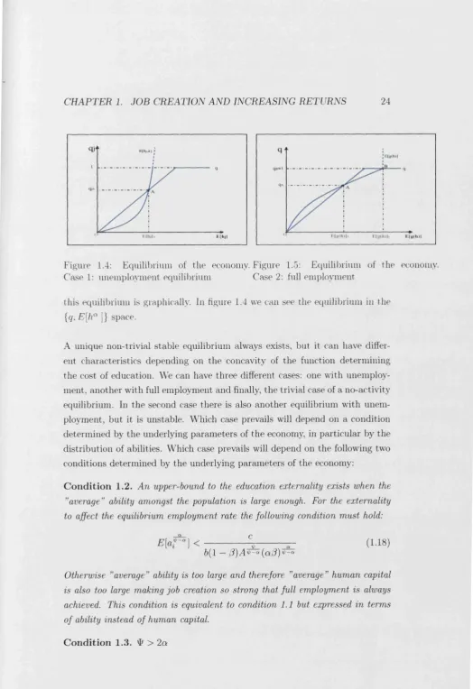
Figure 1.4: Equilibrium of the economy. Figure 1.5: Equilibrium of the economy. Case 1: unemployment equilibrium Case 2: full employment
this equilibrium is graphically. In figure 1.4 we can see the equilibrium in the
{q, E[ha]} space.
A unique non-trivial stable equilibrium always exists, but it can have differ
ent characteristics depending on the concavity of the function determining
the cost of education. We can have three different cases: one with unemploy ment, another with full employment and finally, the trivial case of a no-activity equilibrium. In the second case there is also another equilibrium with unem ployment, but it is unstable. Which case prevails will depend on a condition
determined by the underlying parameters of the economy, in particular by the distribution of abilities. Which case prevails will depend on the following two
conditions determined by the underlying parameters of the economy:
C ondition 1.2. An upper-bound to the education externality exists when the ”average ” ability amongst the population is large enough. For the externality to affect the equilibrium employment rate the following condition must hold:
a C
'' 31 (!-18)
6(1 — /3)A^-a(a/3)^-a
Otherwise ”average” ability is too large and therefore ” average” human capital
is also too large making job creation so strong that full employment is always
achieved. This condition is equivalent to condition 1.1 but expressed in terms of ability instead of human capital.
[image:27.605.27.552.31.796.2]CHAPTER 1. JOB CREATION AND INCREASING RETURNS 25
Figure 1.6: Equilibrium of the economy. Case 3: no economic activity
This makes the second derivative of the ”average ” human capital equation with respect to the employment rate negative. That is, average human capital in
creases less than proportionally when the probability of employment raises. The intuition being that a higher 'ip raises the rate at which the marginal cost of ed ucation increases while the rate at which the marginal benefits of education rises remains constant. Therefore individuals have a lower incentive to invest
in education as the employment rate raises.
A xiom 1.2. The unique non-trivial stable equilibrium can have unemploy ment or not depending on the concavity of the cost of education function, the
distribution of abilities and the exogenous parameters of the economy:
Case 1: if conditions 1.2 and 1.3 hold we have an equilibrium which is stable (point A in figure 1.4). This equilibrium will have unemployment with low ” average” human capital and low market tightness.
q' = Ai ( £ [ a ^ | )
h] =[/ta/JA jaJ1=5 ( ^ [ a 1^ "])* 2°
where A, =
CHAPTER 1. JOB CREATION AND INCREASING RETU RN S 26
(point B in figures 1.5 and A .l).
q2 = 1
h2 = (AapCLi)*^
0} =
In addition, if condition 1.2 is also fulfilled, we have a second equilibrium
with some unemployment and low investment in human capital, but
unstable (figure 1.5, point A).
C ase 3: Otherwise, an equilibrium different from zero does not exist (figure
1.6).
The more interesting is case 1, in which an stable equilibrium with unemploy
ment is obtained. This case results from the existence of a coordination failure
problem, or externality in the accumulation of human capital. This externality results from the interaction between the search frictions in the labor market
(trading externality) and the heterogeneity of individuals. When an individual
(or rather a group of individuals) increases his human capital he knows he will
obtain a higher wage if he finds a job. However, he cannot realize th at the sub sequent rise in the ’’average” level of education will increase expected profits
and job creation, rising the employment rate. It is the failure to recognize this
second effect th at gives rise to the coordination failure. Therefore, if there are
not enough incentives for the individual to invest enough in human capital, the
firm will expect a less qualified worker and its expected profits will decrease,
reducing job creation and the investment in human capital of all individuals. Then the economy may find itself at a situation with high unemployment, and
a low level of human capital.
The intuition for case 3 is the following. When the ’’average” level of ability is
too low or the parameters determining the cost (benefit) of opening a vacancy
are too high (low), firms will have no incentive to open any vacancy and there
will be no activity in the labor market. This corresponds to the case in the
labor market equilibrium, in which the job creation curve has a bigger slope
than the employment rate curve for all 6. This is an interesting result which
CHAPTER 1. JOB CREATION AND INCREASING RETU RN S 27
or in deprived areas within a country.
P ro p o sitio n 1.1. An increase in the education level of some individuals in
creases market tightness and therefore the probability to find a job. This in
creases the expected wage of every individual and thus his investment in human
capital.
Proof: From lemma 1 . 1 we know that the individual’s investment in human
capital increases with the probability to find a job. And from lemma
1 . 2 we know that the value of the market tightness that equilibrates
the labor market depends positively on the ’’average” human capital existent in the economy. Therefore, the individual’s optimal investment
in education depends positively on the ’’average” level of education. This
becomes clear by substituting the employment rate that equilibrates the
labour market (equation 1.13) into the optimal investment in human
capital (equation 1.15).
h i = <
- i f q < 1
^ (A a fia i)* ^ i f q = 1
The equilibrium with unemployment described in case 1 and corresponding
to point A in figure 1.4) is stable. To see why we can think of what would
happen if the economy was below point A, with an employment rate and ’’av
erage” human capital lower than in equilibrium. At that employment rate,
the ’’average” level of education optimal for individuals is higher than the one
which equilibrates the labor market. That is, it is higher than what firms
expected. This implies that too few vacancies are opened and thus the compe
tition between firms for the existing workers is not very intense, which makes
the expected net profits per vacancy positive. Thus the number of vacancies starts augmenting and so does market tightness, increasing the probability to
find a job. This augments the individuals’ incentives to invest in education and eventually improves the ’’average” level of education, which in turn increases
even further the net expected profits of firms. This process goes on until q and
E[ha] rise back to the equilibrium. A similar argument applies for the stability
CHAPTER 1. JOB CREATION AND INCREASING RETURNS 28
Figure 1.7: Case 3: Equilibrium of the economy with compulsory education
E(g(h)]
1.5 and 1.5).
The possibility of the market shutting down when the ” average” level of ed ucation is too low is very worrying. However, this possibility can be reduced
by introducing some compulsory education, so that all individuals acquire a minimum level of education even if there are no job opportunities at all. This is equivalent to assuming that the individually optimum level of investment in
human capital has a lower bound equal to that compulsory education (/imm), which does not affect utility. That is:
hi = { A a p a iq ) ^ + hmin
If we take expectations we get
E[ha ] = (A a P q )* ^ E [ a * ^ ] + hm
This implies that now even in case 3 we can obtain a stable non-trivial equilib rium with unemployment (point A in figure 1.7). This shows that an education policy guaranteing a minimum level of compulsory education for all individ
uals, is not only important because of the individual gains in terms of future
expected earnings but also because it helps to ensure the existence of labour
CHAPTER 1. JOB CREATION AND INCREASING RETU RN S 29
1.5
S o cia l P la n n e r ’s S o lu tio n
The existence of a positive externality from education raises an important
question about the social optimality of the individual decision. Individuals
cannot internalize the externality in their optimal decisions, since they con
sider the employment rate as given, therefore their investment in education
in equilibrium might be different from the socially optimal, and in fact it can be proven to be too low. The social planner knows that the investment de
cisions affect the equilibrium in the labor market, thus he will take this into
account when deciding the optimal investment. He will maximize the following
objective function:
ax | m (0,1)L
J
Ah(a)a f(a)da — cV — LJ —
/ ( a ) d a |max Q i
Solving this problem we obtain the socially optimal market tightness and hu
man capital investment
gSP= ( ^ E [ha\" ^
/ifp = (A a a n fp ) (1.19)
where ^ > 1 > a >0.
P roposition 1.2. The socially optimal investment in human capital is higher than the individually optimal investment.
Proof: Comparing the socially optimal level of investment (h fp ), with the privately optimal level (/if), (equation (1.5)), we have that:
h f P > h> i f f qsp > 0qp
which is always true since qsp > qp in equilibrium (proof in the ap
pendix).
This shows th at there is scope for policy intervention. That is the government
should subsidise individuals’ investment in education to reach the socially op
CHAPTER 1. JOB CREATION AND INCREASING RETU RN S 30
for human capital. An example of the importance of policy intervention was
shown in the equilibrium of case 3 where a policy guaranteing a minimum level of education for every individual made sure that a labour market would always
exist.
1.6
P h y sica l C a p ita l
In this section we consider the investment in physical capital by firms. We
assume that a perfect market for capital exists where capital can be rented
once the match is realized. That is, the capital investment by firms is not
sunk, it can be recovered. The technology of production now will be:
yij - Ak)~ah f
where i represents the individual and j the firm.
The introduction of physical capital in the model generates the following
changes with respect to the basic model. First, the total match surplus now has to take into account the cost of renting the capital. Solving the Nash
Bargaining problem in the same way as in section 1.2, we get the new wage
and profit rules:
Wij = /3(Akj~ah f - rkj) + (1 - (3)z
7n j = (1 - (3)(Ak)-ati* - rkj) - ( 1 - (J)z
Secondly, the firm’s maximization problem has also changed. The firm now has
to undertake two different investment decisions. It has to decide whether to open a vacancy or not, incurring in the sunk costs of advertising and recruiting,
depending on the expected profits from opening it. Then, once the worker has
been recruited, it has to decide what is the appropriate level of physical capital
it needs to rent for the worker’s level of human capital. That is, when the firm
acquires the physical capital it already knows the level of human capital of the
worker. This implies that we can determine the capital decision first, taking
CHAPTER 1. JOB CREATION AND INCREASING RE TU RN S 31
optimal level of physical capital will be equal to:
kj = argmaxTTjj = argm ax(l — (3) (Akj ah\f — rkj — z) given h
and solving we get,
kj — hi A( 1 — a)
This implies that the firm will acquire capital until the physical to human
capital ratio is constant and equal for all firms, so we can drop the subscripts.
A {\ — a)
The wage and profit rules can also be expressed in terms of this ratio:
1—a
wk - aPAh{ + ( 1 - (3)z
n k = a { l - P ) A h i -- ( l - P ) z(1
Now, we can solve the rest of model in the same manner as before. The main difference with the basic model is that all equations will be multiplied by a
factor which is a function of the physical to human capital ratio. The optimal
investment in education by the individual will be:
h? = aA(3diq (
^
1—a
(1.20)
where ^ > 1. And the equilibrium of the economy with physical capital will
be obtained by solving the following system of equations:
E[hk] = [aA0q]*=i £[a*=r] ( -1 —a
k \
* - »[a © I" 0 ] 1
1 otherwise
CHAPTER 1. JOB CREATION AND INCREASING RETU RN S 32
equations. Now the externality of education is potentiated by firms’ invest
ments in physical capital. As in the basic model, when some individuals invest
more on education, they raise the economy’s average level of education and
the expected profits of firms from opening a vacancy. Increasing job creation
and the probability of employment for all individuals. However, now we have
a second mechanism. The firms matched with these more skilled individuals will invest more on capital, increasing even further the gains from the match.
This provides an additional incentive for all individuals to invest in education. Now it is the exact average level of education what affects the employment
rate, which is larger than the ’’average” human capital of the basic model
(E[hi\ > E[hf since a < 1). The effect will be potentiated even further if the
physical to human capital ratio is larger than one. This will happen when the cost of renting capital is low, and/or the technological level and the share of
physical capital in production are high. The reason being that in this case for
every unit of human capital the individuals contribute to the match, the firm
contributes with more than one unit of physical capital.
W ith capital, the conditions for an equilibrium with unemployment to exist
are slightly different:
E h * - 1] < c (1.21)
b(1 — (3)A^~a (aP)^~a
V > 2 (1.22)
A xiom 1.3. A stable equilibrium with unemployment exists if both conditions
hold equal to the following:
CHAPTER 1. JOB CREATION AN D INCREASING RETU RN S 33
1.7
D ifferen t U n e m p lo y m en t R a te s
It is a known stylized fact th at individuals with higher levels of education
face lower unemployment rate and this empirical fact seems to hold for most
developed countries and education levels 6. Mincer (1991) suggests that the
differences in individual unemployment rates are mainly due to the fact that more educated workers are relatively more efficient in acquiring and processing
job search information and that workers and firms search more intensively to
fill more skilled vacancies. In this section I try to reconcile the basic model
with this empirical fact by endogeneizing the individual’s search efficiency. 7
The basic model in this chapter assumes that all individuals face the same unemployment rate, this is because they all search with the same intensity.
Instead, we may think that different individuals search with different inten
sity depending on their characteristics. The more intensively an individual
searches, the higher the probability of finding a job. Then, the individual
probability of employment will be equal to the number of search units th at particular individual supplies (s*) times the general employment rate prevail
ing in the economy. And the same will be true for the probability of filling a
vacancy with individual i. Namely,
Qi = s{q
Pi = Sip
The aggregate supply of search units (S) will be the sum of the efficient search
units supplied by each individual:
S =
J
sf(s)d sIn this case, each person has to make two decisions: the investment in edu
cation and the number of units of search to supply. It is assumed th at the
acquisition of s* units of search and hi units of education, requires an effort e*,
which is increasing in the amount of education or search units acquired and
decreasing in the ability of each individual. A simple expression th at satisfies
6In some developing countries, like India, this is not true
CHAPTER 1. JOB CREATION AND INCREASING RETU RN S 34
these assumptions is:
Therefore, the individual will solve the following maximization problem:
ti? sT
maxm = PAhfSiq
---h i , s i C ljl
Solving, we obtain the optimal search intensity as a positive function of educa
tion and the investment in education as a positive function of search intensity,
while both are a function of ability and the employment rate.
hi = (aAftdiSiq)*-* (1-23)
Si = (A fia ihfq)*^ (1-24)
where > 1 > a > 0 and T >1.
The main difference with the basic model in the labor market is th at now we
have L workers, supplying S units of search, and V firms who engage in a
search process. That is, we have to redefine the market tightness as the ratio
of vacancies to the total supply of units of search: 0 — Solving in the same manner as in the basic model we get the ” Job Creation Condition” and the
” Employment Rate Condition” :
o _ ( f s ( a) h( a) af ( g) da
[ c J f s ( a ) f ( a ) d a
f s ( a ) h ( a ) a f ( a ) d a j i-<t> ^ ^ 0 ) ^ < 1
q = I
(1.25)1 o th erw ise
Then, the individual’s probability of employment will be (if (b d < 1):
9i = Si<? = ( j H a m ^ ) " * { W
(1.26)
CHAPTER 1. JOB CREATION AND INCREASING RETU RN S 35
effect there is another effect due to the search efficiency. When some individuals
invest more in education, they increase the average level of education, but
they also become more efficient in searching, rising aggregate search efficiency.
This will increase expected profits per opened vacancy since firms now have
a higher probability of finding those more skilled individuals and job creation
goes up. However, at the same time, this has a negative effect on the rest of individuals searching for jobs, since they are now relatively less efficient in
searching and therefore face higher unemployment rates. That is, a rise in
average education generates two effects. On the one hand, it increases job
creation, but at the same time it increases aggregate search efficiency reducing
everyone else’s chances of finding a job.
1.8
C o n clu sio n s
The main contribution of this chapter is to develop a theoretical model showing
how an education externality might be generated exclusively from the process
of matching in the labour market without the need of increasing returns to
scale neither in the production function nor in the matching function. It is the interaction between the ex-ante decision to invest in education by workers
and to open a vacancy by firms that gives rise to the externality. The model
shows that when the economy is in an equilibrium with unemployment due to
the education externality there is a connection between aggregate employment
(or unemployment) and the distribution of education in the labour force.
The existence of the externality means that there is scope for intervention.
Individuals cannot internalize the effect the externality has in their optimal
decisions, since they take the employment rate as given, and therefore their
equilibrium investment in education is lower than the socially optimal. This
is particularly interesting in the case in which an economy finds itself in an
equilibrium with no activity due to the low level of skills of its population. A
clear example of this are the labour markets in many developing countries or
the lack of specialized labour markets in certain areas of developed countries.
The model developed in this chapter indicates that a solution to this problem
might be to implement an education policy which guarantees a minimum level
CHAPTER 1. JOB CREATION AND INCREASING RETU RN S 36
population enough to provide incentives for firms to start creating vacancies
in that area (or particular sector) and for workers to invest in education above
the compulsory level. Eventually, both these forces will take the economy into
an equilibrium with economic activity, reducing aggregate unemployment.
Finally, the theoretical model is extended to consider the effect of having phys ical as well as human capital. The introduction of both types of capital is
shown to potentiate the education externality. Now in addition to the standard
mechanism, by which a rise in the education investment of some individuals
increases expected profits per vacancy and job creation, we have a second one.
The firms matched with these more skilled workers will also invest more in capital increasing even further the gains from the match and providing with
an additional incentive for workers to invest more in education.
The model is also extended to consider the possibility that different individ
uals face different unemployment rates, depending on their search efficiency, which is a function of ability. This will potentiate the effect of the externality
for these individuals who have increased their education, but it will dampen
it for the rest of individuals. The reason being that when some individuals
increase their education, they improve the average level of education in the labour market, which has two opposite effects: it increases job creation, but at
the same time it increases aggregate search efficiency reducing everyone else’s
chances to find a job.
Some of the interesting further work to be done in this area would consist in
extending this model to consider other related mechanisms, like the possibility
of migration between regions, which is studied in chapter 2. In addition, an empirical test of the empirical relevance of this mechanism is necessary. Two
C hapter 2
E d u cation m atch in g
ex tern a lities and th e lo ca tio n o f
econom ic a c tiv ity
2.1
In tr o d u c tio n
The analysis of the concentration of economic activity in specific geographic
areas has been a very dynamic area of research since the seminal papers by
Krugman (Krugman (1991a), Krugman (1991b)). But, as Krugman himself
states, the basis of this analysis was developed much earlier. Alfred Marshall (Marshall (1920)) already identified three reasons to explain the concentra
tion of economic activity in a certain geographical location: pooling of skilled
workers, input-output linkages and technological spill-over effects. So far, this
literature has centered its attention on the existence of pecuniary externalities
in the production process, coming mainly from Marshall’s second and third reason for concentration, but little attention has been paid to the first one. In
general, these models have given a secondary importance to the labor market
and the accumulation of skills. An exception being Rotemberg and Saloner
(2000). They develop a model th at explains concentration based on the ex
istence of an externality coming from the supply of workers with the specific skills required by the industry. In their model, workers will only be willing to
acquire these specific skills if there axe enough firms wanting to employ them
and vice-versa. But they concentrate on specific skills and do not consider the existence of unemployment, while most empirical studies show th at this is
one of the most important determinants of regional migration (see Greenwood
CHAPTER 2. LOCATION AND MATCHING E X TE RN ALITIE S 38
(1997)).
In addition, the analysis of the relationship between labor markets, skill ac
cumulation and geographic concentration of economic activity seems specially
relevant since differences across geographical areas in unemployment rates and
average human capital are large and persistent for most developed countries.
In this chapter we propose a mechanism by which geographical concentration of economic activity may arise from a pecuniary externality originated exclu
sively in the labor market

![Figure 1.3: Rise in E[ha]. Case 2: 0max > |](https://thumb-us.123doks.com/thumbv2/123dok_us/454405.1045105/26.606.33.547.26.810/figure-rise-in-e-ha-case-max.webp)