Munich Personal RePEc Archive
Human activities and global warming: a
cointegration analysis
Liu, Hui and Rodríguez, Gabriel
University of Ottawa
2005
Online at
https://mpra.ub.uni-muenchen.de/9939/
Human activities and global warming:
a cointegration analysis
*
Hui Liu, Gabriel Rodrı´guez
*
Department of Economics, University of Ottawa, P.O. Box 450, Station A, Ottawa, ON, Canada K1N 6N5
Received 25 July 2003; received in revised form 22 February 2004; accepted 30 March 2004
Abstract
Using econometric tools for selecting I(1) and I(2) trends, we found the existence of static long-run steady-state and dynamic long-run steady-state relations between temperature and radiative forcing of solar irradiance and a set of three greenhouse gases series. Estimates of the adjustment coefficients indicate that temperature series is error correcting around 5e65% of the disequilibria each year, depending on the type of long-run relation. The estimates of the I(1) and I(2) trends indicate that they are driven by linear combinations of the three greenhouse gases and their loadings indicate strong impact on the temperature series. The equilibrium temperature change for a doubling of carbon dioxide is between 2.15 and 3.4(C, which is in agreement with past literature and the
report of the IPCC in 2001 using 15 different general circulation models.
Ó2004 Elsevier Ltd. All rights reserved.
JEL classification:C22; Q00
Keywords:Global warming; Radiative forcing; Cointegration; I(1) process; I(2) process; Unit roots
1. Introduction
One of the main conclusions achieved by the Intergovernmental Panel on Climate Change (IPCC, 2001) is that temperature series is warming for the past 150 years. Furthermore, the same reference attributes the responsibility of the changes to human activities generated greenhouse gases. A basic argument in this diagnostic is that temperature series are higher com-pared to the pre-industrial periods; see alsoSanter et al. (1996). There are two sources for this evidence. They are the physically-based simulation models of climate and the statistical analysis of historical data, respec-tively. The simulation models of climate are based on physical motion equations trying to describe the princi-pal issues governing the behavior of temperature. They also include the radiative forcing of greenhouse gases
and tropospheric sulfates. This kind of model are gen-erally referred as general circulation models (GCMs).
On the other hand, the statistical analysis deals directly with the historical record of the temperature variables, solar irradiance and greenhouse gases. In some cases, this approach uses simple and standard statistical or econometric tools in identifying for the effects of human activities (greenhouse gases) on the temperature series. However, because all these time series exhibit strong trends, classical tools will indicate spurious positive relation among these variables. In consequence, it is important to identify clearly the time series properties of the data before starting any other kind of analysis between the series. In this aspect, the principal goal is the identification for the existence of unit roots in the data which means the existence of stochastic trends. It is the starting point of the research agenda ofStern and Kaufmann (1997, 1999, 2000)and
Kaufmann and Stern (2002).1Using different statistical
www.elsevier.com/locate/envsoft
*
This paper is drawn from the first chapter of the Ph.D. dissertation of Hui Lui at the University of Ottawa.
* Corresponding author. Tel.:C1-613-562-5800; fax:C 1-613-562-5999.
E-mail address:[email protected](G. Rodrı´guez).
1
See next section for a brief but more complete survey of the literature.
tests for the identification of unit roots, they find that temperature series is an I(1) process,2 and that green-house gases contain two unit roots. After analyzing for causality between different set of time series,Stern and Kaufmann (1997) investigate the existence of long-run steady-state relations (i.e. cointegration between sets of variables) using multivariate techniques proposed by
Johansen (1988, 1995b). They conclude that there exists a long-run relation between the set of variables and that temperature series is reacting to the disequilibria towards this steady-state relation in around 40e50% each year. However, the authors believe that this value is too high and it may be a consequence of the existence of I(2) trends in the system. Kaufmann and Stern (2002)
recognizes the necessity to take into account for I(2) trends in an adequate statistical framework.
The statistical framework for I(2) is proportionated by the approach suggested by Johansen (1992, 1995a); see also Paruolo (1996); Rahbek et al. (1999);Paruolo and Rahbek (1999). It is more complex but richer in terms of the long-run relations that we may find. In fact, there are the standard (static) long-run steady-state relations but there also exist the dynamic long-run steady-state relations which are given by the linear combinations between the levels of the variables and their first differences. It is also possible to find medium-run steady-state relations. In this paper, we follow this approach.
The empirical results show that global temperature and solar irradiance series are I(1) processes, carbon dioxide is an I(2) process, and methane and nitrous dioxide seem to contain explosive roots. According to this evidence, three different systems are proposed, estimated and analyzed. The results indicate that temperature series is error correcting around 10e50% of the disequilibria each year, depending of the type of steady-state relation that is considered. Regarding the equilibrium temperature change for a doubling of carbon dioxide, the results indicate that it is between 2.1 and 3.4 (C, depending of the steady-state used to
calculate it. It is worth noting that these values are in agreement with other values found in the literature (see
Kaufmann and Stern, 2002) and the average value calculated by the Intergovernmental Panel on Climate Change (IPCC, 2001).
The rest of this paper is organized as follows.Section 2presents a brief review of the literature.Section 3deals with the methodological issues whileSection 4presents the empirical results.Section 5concludes.
2. A brief review of the literature
In order to place this work in the context of the literature on climate change, a brief summary of some of the relevant papers is provided below. When we observe pictures of global temperature series, greenhouse gas concentrations, and solar irradiance, all give us the information that they have increased in the last 150 years; see alsoStern and Kaufmann (2000). Presence of strong trends implies that the use of standard statistical or econometric tools will indicate a significant and positive association between sets of variables analyzed. Unfortunately, the use of standard statistical or eco-nometric tools is misleading in this context. Therefore, a careful analysis of the statistical properties of the time series appears as a necessary condition for an adequate empirical analysis. This is the starting point of the research applied by Stern and Kaufmann (1997, 1999, 2000), and Kaufmann and Stern (1997, 2002). Apart from them, there is little research that explicitly argued in favor of the use of econometric time series methods, such as Tol (1994), Tol and de Vos (1998), and Scho¨nwiese (1994). Some other exceptions in the anal-ysis of the time series properties of global temperature series are Bloomfield (1992), Bloomfield and Nychka (1992), Woodward and Gray (1993, 1995), Galbraith
and Green (1993); Richards (1993); Fomby and
Vogelsang (2002). Before them, most of the research analyzing the relationship between temperature and forcing variables have used simple regression models as inLean et al. (1995), or frequency domain methods as in
Kuo et al. (1990)andThomson (1995, 1997).
The analysis of the time series properties of tempera-ture, solar irradiance, greenhouse gases and other variables has been performed in Stern and Kaufmann (1997). One of the principal conclusions of their research is that global temperature series has a unit root or in other terms, this time series has a stochastic trend, which is denoted by I(1). At the same time, greenhouse gases variables have been found to contain one or two unit roots. The econometric tools used were the well known unit root statistics proposed byDickey and Fuller (1979), Said and Dickey (1984), Phillips and Perron (1988), and
Schmidt and Phillips (1992). As a consequence of the size and power problems of these unit root statistics in detecting for more than one unit root,3 there is not a complete and clear picture regarding the degree of integration of the greenhouse gases. However, the evi-dence in favor of two unit roots is present in more than one unit root test. It is also recognized inStern and Kaufmann (1999, 2000), andKaufmann and Stern (2002).
When the time series are non-stationary there is room to test for cointegration, that is, the possible existence of
2A time seriesytis integrated of orderd, which is denoted by I(d) if
ddifferences are needed to transform it into a stationary time series. Therefore, I(1)/I(2) means that the series has to be differenced one/two
long-run relationships between sets of variables ana-lyzed. In other words, it is possible to find linear combinations of the variables that annihilates the stochastic trends. The rest of linear combinations are still stochastic trends and they drive the behavior of the time series. The cointegrating relations are named also static long-run relations because they represent a steady-state relation between sets of variables. Because in the short term the variables are not in the steady state, they will react to these disequilibria. In the case of tem-perature, for example, it is possible to find a steady-state relation with greenhouse gases and natural factors (solar irradiance, for example). In the short term, the tem-perature (and the other variables) reacts to the dis-equilibria exhibiting an error correction behavior.
The only two trials to deal with the identification of cointegration relations have been Stern and Kaufmann (1997) and Kaufmann and Stern (2002). Using the methodology ofJohansen (1988, 1995b),4they arrive at the conclusion that there exists a long-run relationship between time series of temperature, solar irradiance and a set of greenhouse gases. The estimates of the short-run dynamic model indicate that temperature is correcting around 40e60% of the disequilibria each year. The authors consider that this value is too high and they attribute its cause to the existence of I(2) trends.
The acceptation that time series of greenhouse gases contain I(2) trends is also present in Stern and Kaufmann (1999, 2000). In both papers, the authors apply a multivariate structural time series approach to model temperature, natural factors and greenhouse gases.5 The advantage of this kind of models is that different alternatives for the deterministic components are allowed. Also, it is possible to allow for I(1) and I(2) trends. The model is also flexible in including cyclical components. The basic conclusions are that most time series analyzed contain a stochastic trend with the greenhouse gases containing stochastic I(2) trends. Therefore, the two independent stochastic trends in the data are associated to the radiative forcings due to greenhouse gases, solar irradiance, and tropospheric sulfate aerosols that are found in the northern hemi-sphere, respectively. More recent research but applied to the temperature of Australia is Lenten and Moosa (2003). According to their results, temperatures in six Australian locations are I(1) processes, the cyclical component is not significant, seasonality is deterministic and the irregular (or noise) component is very significant. On the other hand, some different results are proportionated by Kelly (2000). He finds that temper-ature series contains a unit root but that greenhouse
gases are stationary around a time trend. This impres-sive result implies that temperature rise is due to long run cycles, and that the relationship with greenhouse gases is spurious. These results are in complete opposition to most of the research detailed before. However, applying first difference to temperature series,
Kelly (2000) estimated a regression between growth rates of temperature and greenhouse gases, finding support to previous results regarding the significant influence of these gases on temperature series.
One important and uncertain parameter of the general circulation models (GCMs) is the temperature sensitivity which is measured as the equilibrium temperature change per unit of the change in radiative forcing. AsKelly (2000)argues, an alternative measure, directly proportional to the climate sensitivity, is the total equilibrium (steady-state) temperature change from a doubling of greenhouse gases, frequently denoted as DT2x.Kelly (2000)finds that this parameter
is between 1.27 and 1.33 (C; while forKaufmann and
Stern (2002) its value is around 2.0 and 2.5 (C, in
agreement with the general circulation models. It is worthwhile to mention that theIPCC (2001)argues that the average value of DT2x is 3.5 (C after considering
15 different models.6
In this paper we still use time series tools to analyze for the existence of steady-state relations between temp-erature series, solar irradiance and a set of greenhouse gases. However, unlike the traditional approach of using the so called I(1) model, asStern and Kaufmann (1997) and Kaufmann and Stern (2002), we use econometric tools allowing for the presence of I(2) trends in the identification of the long-run relationships. The use of more sophisticated econometric tools taking into ac-count for the presence of I(2) trends has been recognized by Stern and Kaufmann (1999). The presence of two unit roots in time series allows us to use the so called I(2) model (seeJohansen, 1992, 1995a, 1995b). In this model the number of cointegrating relations are detected, so are the number of I(1) and I(2) stochastic trends that still in the system and drive the behavior of some variables. In terms of the cointegrating relations, unlike the analysis of the I(1) model, the I(2) model allows for the existence of two types of cointegration. The first type is a linear combination of the variables in their levels, which is the same definition as that in the I(1) model. The second type of cointegration is the possibility that there are linear combinations between the levels of the variables and their growth rates. It is named polynomial cointegration and also dynamic steady-state relations. Further details of I(1) and I(2) models are presented in the next section.
4See the I(1) model below for further methodological details. 5
This methodology is based on Harvey (1989).
6
The standard deviation is 0.92(C and the range goes from 2.0 to
3. Methodological issues
In this section we provide elements relevant to under-standing the methodological approach applied in the empirical analysis. Regression with nonstationary time series implies spurious regression except when there exists a linear combination (or more than one) between these variables that reduce the dimension of the space spanned by them. This is known as cointegration.
3.1. The I(1) model
Letyt, a vector containingnvariables, be represented
by the followingVAR(k):
yt ¼
Xk
i¼1
PytiCFDtC3t ð1Þ
where it is assumed that 3t is a sequence of i.i.d. zero
mean with covariance matrixU. In most cases it is also
assumed that the errors are Gaussian which is denoted by 3twN (0,U). The variable Dt contains the possible
deterministic components of the process, such as a con-stant, a time trend, seasonal dummies and intervention dummies. This is the model proposed by Johansen (1988, 1995b) and is widely used in empirical applica-tions.7
The system (1) is reparameterized as a vector error correction model (VECM):
Dyt¼Pyt 1C
Xk1
i¼1
GiDyt
iCFDtC3t ð2Þ
with
P¼ ICX
k
i¼1
Pi; Gi¼ X
k
j¼iC1
Pj:
Notice that the matrix
G¼IX
k1
i¼1
Gi:
I(1) cointegration occurs when the matrix P is of
reduced rank, r!n where P may be factorized into P=ab#, a and b are both full rank matrices of
dimension n!r; the matrix a contains the adjustment coefficients and b the cointegration vectors. These vectors have the property that b#yt is stationary, even
thoughytitself is non-stationary. Notice that there also
exist full rank matrices at and bt of dimension
n!(nr) which are orthogonal to a and b, such that a#ta=0 andb#tb=0, and therank(bt,b)=n.
An alternative representation of the cointegrated VAR model is in terms of the common stochastic trends representation, seeStock and Watson (1998). According to that, theytvector is represented by
yt¼FDtCC
Xt
i¼1
3iCCðLÞ3t ð3Þ
where C=bt(a#tGbt)
1
a#tandC(L)3tcorresponds to
a n-dimensionalI(0) component. Using this representa-tion it is possible to observe that although yt is
n-dimensional, the vector series is driven by just nr
common stochasticI(1) trends which are
a#t Xt
i¼1
3i:
In terms of observable variables the I(1) directions are calculated as b#tyt which are just a particular linear
combinations of the stochastic trends.
To test the rank of matrix P, Johansen (1995a,b)
developed maximum likelihood cointegration testing method using the reduced rank regression technique based on canonical correlations. The procedure consists of obtaining ann!1 vector of residualsr0tandr1tfrom
auxiliary regressions (regressions of Dyt and yt1 on
a constant and the lagged Dyt1.DytkC1). These
residuals are used to obtain the (n!n) residual product matrices:
Sij¼ ð1=TÞ
XT
t¼1
ritr#it; ð4Þ
for i, j=0, 1. The next step is to solve the following eigenvalue problem
KlS11S10S1
00S01K¼0 ð5Þ
which gives the eigenvalues ˆl1R.Rlˆn and the
corre-sponding eigenvectors ˆb1 through ˆbn, which are also the cointegrating vectors. A test for the rank of matrix P can now be performed by testing how many eigenvalues l equals to unity. One test statistic for the resulting number of cointegration relations is the Trace statistic (see Johansen, 1988), which is a likelihood ratio test defined by
Trace¼ T X
n
i¼rC1
logð1lˆiÞ ð6Þ
Another useful test is given by testing the significance of the estimated eigenvalues themselves
lmax¼ Tlogð1lˆiÞ: ð7Þ
In trace test, the null hypothesis isr=0 (no cointegration) against the alternative hypothesis thatrO0 (cointegra-tion). Thelmaxstatistic tests the null hypothesis thatr=r0
versus the alternative hypothesis that r=r0C1, where
7There are large number of empirical applications using this
r0=0, 1,., n1. For further details regarding the
construction of these statistics, seeJohansen (1995b). In summary, the I(1) model allows to identify the rank of cointegration (r) and the number of stochastic trends driving theytvector. Because in this model it is
assumed thatytcontains variables with order of
integra-tion no larger than one, it is clear that the number of unit roots left in the system is nr. Notice that the estimate ofb(the cointegration vector) is not identified in the sense that any linear combination of b is also a cointegration vector. In this sense, researchers have to identify these vectors by imposing restrictions that are in most cases suggested by the economic theory. For example, in a vector containing four variables, a possible restriction is that the coefficient associated to the second variable is zero. If the statistic (distributed as ac2) does not reject the null hypothesis, it means that the second variable is long-run excluded from the cointegration vector. Another example is the restriction of long-run homogeneity between a set of variables. If the null hypothesis is not rejected, it means that the unit vector (i.e. [1, 1,., 1]) may be used in the subsequent
analysis. The estimated adjustment coefficients (a) are also tested for restrictions but in this case, the restrictions are associated with the null hypothesis of weak exogeneity.
3.2. The I(2) model
In the I(1) model, the matrixPis of reduced rank and
the matrixa#tGbtis of full rank. For the system to be
I(2) it is also required that the matrix a#tGbt be of
reduced rank s1!nr. Following Johansen (1992, 1995a,b), the model (2) can be reparameterized as
D2yt¼Pyt1GDyt1CX
k2
i¼1
JiD2ytiCFDtC3t ð8Þ
where the matrixGis included as a parameter and
Ji¼ X
k1
j¼iC1
Gj:
With the matrix a#tGbt of reduced rank (sq), it is
possible, as in the I(1) model, to define parameter matrices x and h such that the second reduced rank condition isa#tGbt=zh#withzandhboth matrices of
dimension (nr)!s1.
As in the I(1) model, the number of cointegration relations (or I(0) relations) is denoted by r. However, unlike I(1) models, nr does not only represent the number of I(1) trends in I(2) models. It contains both the total of I(1) trends and that of I(2) trends, denoted as
s1and s2, respectively. Consequently there are param-eters describing the I(0), I(1) and I(2) directions of the
variables and an important goal of the I(2) model is their identification. Following the notation ofJuselius (1999), these matrices are b, bt1 and bt2 associated with
dimensionsr, s1 andnrs1=s2respectively.8Paruolo (1996) denotes r, s1, s2 as the integration indices of the VAR.
In a similar way as in the I(1) model, the common trends representation of I(2) model is given by
yt¼FDtCC2
Xt
j¼1
Xj
i¼1
3iCC1
Xt
i¼1
3iCCðLÞ3t ð9Þ
whereC2¼bt2ða#t2Qbt2Þ
1
a#t2andC*(L) is a matrix
polynomial with all roots strictly outside of the unit circle. The first clear observation is that yt has s2
common I(2) trends given by
a#t2X t
j¼1
Xj
i¼1
3i:
In terms of observable variables, it is given by b#t2yt
which are just linear combinations of the I(2) stochastic trends.
Furthermore, as mentioned by Haldrup (1999), the combinations b#yt can cointegrate to I(0) level and/or
have the property that they potentially cointegrate with b#t2Dyt, which is I(1) by construction. This is named as
polynomial cointegration. These r relations are b#yt
db#t2Dytwhich define the I(0) directions. However, not
all the rI(0) relations need include the differenced I(2) components. In fact, after definingdtsuch thatd#td=0,
there will be rs2 non-polynomially cointegrated relations given byd#tb#yt; ands2polynomial
cointegrat-ing relations given byd#b#ytd#db#t2Dyt.9
The approach suggested by Johansen (1992, 1995b)
to identify the number of I(2) trends is conducted as a combination of regression and reduced rank re-gression. It is performed in a similar way as the deter-mination of the cointegration rank in the I(1) model. The difference is that now two reduced rank conditions need to be examined. This is more complicated in the sense that the second reduced rank condition depends on the first reduced rank condition. Instead of a joint
8
The notation and technical details of the I(2) model are complex. Further details regarding the calculation of matricesbt1andbt2are
in Juselius (1999), also Haldrup (1999) using a slightly different notation. In summary, becausezandhexist, their complements,zt andht, also exist. Then it is possible to defineatZ{at1,at2} and btZ{bt1, bt2}, where at1Zat(at#at)
1
z at2Zatzt, bt1Z bt(bt#bt)
1
h and bt2Zbtht. Therefore, b, bt1 and bt2 are
mutually orthogonal and thus jointly describe a basis for the
n-dimensional space. Theahas a similar property.
9The possibility to decomposer(inr
0andr1, say) exists only whenr
Os2. In this case, the rcointegrating relations can be divided into r0Zrs2directly stationary CI(2,2) relations andr1Zs2polynomially
estimation of the indicesrands1,Johansen (1992, 1995a)
suggests a two step procedure. The first step is to solve the reduced rank problem associated with the matrix
P=ab#. It calculates the estimates of ar, br, atr, and
btr for each value ofr=0, 1,.,n1. The second step
deals with the second reduced rank condition problem by replacing the unknown matricesatr, andbtrwith the
estimates from the first step. The problem is solved for or
s1=0,.,nr1. Then what remains to be determined is
which combinations ofrands1should be chosen. Because steps 1 and 2 proportionate an array of different values forr ands1corresponding to different sub-models, the selection ofrands1can be performed in the following way.10The array is read starting from the left corner. If the null hypothesis is rejected, the next element (continu-ing to the right) is read and so on. After the first row is done, and if no acceptation is observed, we read the second row of the array. We continue until the first non-rejection is found. The associated values ofr, s1ands2are selected as the integration indices. Complete technical details can be found inParuolo (1996); Johansen (1992, 1995a).
It must be emphasized that only the space spanned by the cointegrating vectors is identified; the single cointe-gration relations are unidentified. This issue is also present in the I(1) model but this problem is more complex in I(2) models.11
What is perhaps more interesting is the fact that in an I(2) model there exist more than one steady-state rela-tions. Recall that in an I(1) models, the cointegration relationsb#ytrepresents the static long-run steady-state
relation. In the present case, we have two additional steady-state relations. One is medium-run steady-state relations represented by b#t1Dyt. The other is dynamic
long-run steady-state relations represented by the poly-nomially cointegrating relations (seeJuselius, 1999, 2003). In consequence, there exist different adjustment coeffi-cients associated with each of these steady-state relations. One should keep in mind that tools for analyzing I(2) models and statistics used to select integration indexes are not yet fully developed in econometric literature. This is the reason why the selection of the number of I(2) trends should be combined with other tools. One of them, as suggested byJuselius (1999), is the calculus of the roots of the companion matrix. Ifytvector contains
variables that are integrated no more than order one, then the total number of unit roots (or close to the unit circle) of the companion matrix must be nr. If there exists more than nr roots close to the unit circle, it
constitutes a indicator for the presence of I(2) trends. When there are I(2) trends, the number of roots close to the unit circle iss1C2s2.
Another useful indicator for the presence of I(2) trends is to compare the graphs ofb#ytandb#R1t, where
R1t is a vector of residuals from regressing yt1 on
lagged short-run effects (Dyt
i,i=1, 2,.,k1) andDt.
If the first graph looks non-stationary whereas the second graph looks stationary, it can be considered as a strong support for the presence of I(2) trends.
Recently a few empirical applications in the field of economics have used the I(2) framework. Without the intention to be exhaustive, some of these references are
Rahbek et al. (1999), Kongsted (2003), Holtemo¨ller (2002), Vostroknutova (2003), Juselius (1999, 2003), Fiess and MacDonald (2001), and Haldrup (1999). It is worthwhile to mention that some of these papers, after identifying for the presence of I(2) trends, proceed with transforming the variables in such a form that a standard I(1) analysis can be performed (seeFiess and MacDonald, 2001). Almost all references mentioned study nominal variables such as money supply, nominal wages, and fundamentally prices. We do not know that a similar methodology has been applied to climate series.
4. Empirical analysis
4.1. The data and preliminary issues
The data used in this paper include the time series of global mean temperature deviation (denoted by temp), the concentrations of methane (ch4), nitrous dioxide (n2o), carbon dioxide (co2).12All data are from the web site of Goddard Institute for Space Studies available at
http://www.giss.nasa.gov. The data are transformed into radiative forcing,13 which affects the temperature
10The test statistic is denoted asHr,sand it is the same notation
used in the empirical analysis.
11Regarding the adjustment coefficients, for example, the notion of
weak exogeneity is now different. Paruolo and Rahbek (1999) have proposed a sequential approach to test for weak exogeneity in the I(2) model.
12A preliminary version of the paper included data of
chlorofluor-ocarbons (cfc11 andcfc12). Graphical inspection of both time series indicates zero values until 1950, after what they increased very fast. These two variables were found to be I(2) processes in Stern and Kaufmann (2000). We decided exclude both time series for the following reasons: (i) the visual analysis indicates a particular behavior that may distort the analysis; (ii) their importance in terms of all greenhouse is reduced; (iii) increasing the dimension of the system of equations to be estimated, therefore reducing the number of freedom degrees given our sample size; and (iv) identification of cointegration relations is complex and unlike the field of economics, we are not sure what are the physical relationships and interactions between all these greenhouse gases series, solar irradiance and temperature time series. Therefore, by excluding both variables, we reduce the possibility to find too many cointegration relations which are always difficult to identify and interpret.
13Radiative forcing is the change of the net irradiance caused by
directly and indirectly. The formulae are tabulated in the Intergovernmental Panel of Climate Change (IPCC, 2001). Therefore the radiative forcing of greenhouse gases at timetare denoted byr f ch4t, r f n2ot, r f co2t. We
also include radiative forcing of solar irradiance (r f sunt)
as another variable in the system.
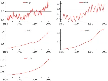
Fig. 1presents the evolution of the time series for the period under study, 1856e2001. It is a similar period as analyzed by the previous literature but with more recent information. A clear observation appearing fromFig. 1
is the fact that all greenhouse gases variables present strong upward trends that have been observed in the previous literature.
As that argued in the literature (Stern and Kaufmann, 2000), an essential preliminary step in the analysis of these variables is the identification of the time series properties. One way to approach this issue is the application of univariate unit root tests. Stern and Kaufmann (2000) proceeded using three different uni-variate unit root tests. However, as documented by
Haldrup and Lildholdt (2002), these statistics are incorrect. Because when testing for I(2) and the un-derlying series is indeed integrated of order two, these statistics give rise to an excessive rejection of the null hypothesis of a unit root in favor of the stationary and explosive alternatives. This size distortion is caused by the fact that the test statistics have a different dis-tribution originated by one additional unit root. In consequence, the recommendation of Haldrup and
Lildholdt (2002) is to test I(2) against I(1) prior to testing I(1) against I(0). The authors conclude that all basic univariate unit root tests suffer from this issue.
In a set of results not reported here,14we applied the approach suggested by Dickey and Pantula (1987) and also the statistic proposed byHasza and Fuller (1979). The results indicated that the carbon dioxide series contains two unit roots, that is, it is an I(2) process. The temperature and solar irradiance series were found to be I(1) processes, the other greenhouse gases series under study (nitrous dioxide and methane) appeared contain-ing explosive roots. The last result is not totally clear after the application of all statistics. The difficulty with this case is the fact that explosive roots mimic the behavior of I(2) processes, see Haldrup and Lildholdt (2002).
In summary, most of the results confirm the previous results found in the literature, seeStern and Kaufmann (2000). Although it appears to be the case, we adopt another strategy in this paper. This approach consists of applying multivariate techniques to detect the number of I(0), I(1) and I(2) trends in the system. As we will see in
1850 1900 1950 2000
-0.5 0.0
0.5 temp
1850 1900 1950 2000
-0.2 -0.1 0.0
0.1 rfsun
1850 1900 1950 2000
0.5 1.0
1.5 rfco2
1850 1900 1950 2000
0.2 0.4
rfch4
1850 1900 1950 2000
0.05 0.10
[image:8.595.117.473.69.334.2]0.15 rfn2o
Fig. 1. Global temperature deviations (temp), radiative forcing of solar irradiance (rfsun), carbon dioxide (rfco2), methane (rfch4) and nitrous dioxide
(rfn2o); units inWm 2
; 1856e2001.
14But they are available upon request. We applied standard ADF
the next analysis, there are more than one possible case in the selection of the integration indices.15
4.2. The first case
The first case is represented by the system with our five variables, i.e.,yt={tempt, r f sunt, r f co2t, r f ch4t,r f
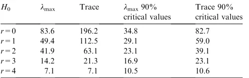
n2ot}. Table 1 presents the results obtained from the
application of the approach of Johansen (1988, 1995b)
in determining the rank of matrixP16. Both Trace and
lmaxstatistics indicate thatr=3, that is, there exist three
cointegration relations. Because n=5, we have
s1Cs2=nr=2.
Table 2 presents the results of the statistic Hr,s for
selecting s2. The first row represents the value of the statistic, the second and third rows are the critical values at 95.0% and 97.5% (in italics). As we explained in the previous section, reading of this table starts from the left-corner and we continue to the right. If no acceptation is found, we continue to the second row of values (r=1). The procedure stops when a non-rejection is found. In the present case, the results indicate that
s2=0 and consequentlys1=2. Then, there are two I(1) trends and there is no I(2) trends in the system. However, note that using critical values at 97.5%, it is possible to finds2=1 and consequentlys1=1.
As suggested by Juselius (1999), a good way to complement this information is the calculus of the eigenvalues of the companion matrix. The eight largest modules obtained from the unrestricted VAR are: 1.0292, 1.0292, 0.9641, 0.9641, 0.9384, 0.9384, 0.7163, 0.7163. It appears to exist two explosive roots and four eigenvalues close to the unit circle. In other words, there appears to exist four unit roots in the system. Now,
because the first step (in the I(1) framework, seeTable 1) indicatesr=3, we proceed with imposing this restriction and now the eight largest modules of the restricted VAR are: 1.0283, 1.0283, 1.000, 1.000, 0.9378, 0.9378, 0.7179, 0.7179. There are two unit roots as a consequence of the restriction of r=3 but there are two more eigenvalues close to the unit circle. It indicates, again, the existence of four unit roots.17 Remember that in the I(2) framework the total number of unit roots is given by
s1C2s2, which in the present case indicates that s1=0 ands2=2.
In summary, we have some different information using the Hr,sstatistic and the eigenvalues of the
com-panion matrix. We decide to working with both alter-natives. Then, they are r=3, s1=1, s2=1 and r=3,
s1=0, s2=2, respectively. In the following, they are named as Case 1 and Case 2, respectively.
Following the notation used in the previous section,
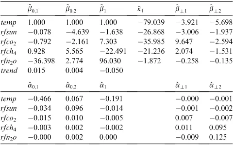
Table 3a presents cointegration relations and adjust-ment parameters corresponding to Case 1. Notice that there are two cointegrating relations including only the levels of the variablesðbˆ0;iyt; i¼1;2Þ:Furthermore, the
relation ˆb1ytkˆ1Dyt denotes the polynomially
cointe-gration relation or what we denoted in the previous section as the dynamic steady-state relation. The bottom panel gives the corresponding loadings ðaˆ0;1;aˆ0;2;aˆ1Þ:
and the coefficients that reflect the composition of the stochastic I(1) and I(2) trends ˆat1 and ˆat2:The table
also presents vectors ˆbt1 and ˆbt2 that denote the
loadings (adjustment parameters) to the stochastic I(1) and I(2) trends.
[image:9.595.311.552.88.270.2] [image:9.595.50.296.91.169.2]Table 3a specifies that around 46.6% of the dis-equilibrium in the static long-run steady-state is
Table 1
Testing for cointegrating ranks
H0 lmax Trace lmax90%
critical values
Trace 90% critical values
r=0 83.6 196.2 34.8 82.7
r=1 49.4 112.5 29.1 59.0
r=2 41.9 63.1 23.1 39.1
r=3 14.2 21.3 16.9 23.1
r=4 7.1 7.1 10.5 10.6
Yt¼ ðtempt;r f sunt;rfco2t;rfch4t;rfn2otÞ#.
Table 2
Testing for integration indices
r Hr,s Qr
0 418.0 312.6 252.0 220.8 198.2 196.2
(198.2) (167.9) (142.2) (119.8) (101.5) (87.2) (203.2) (173.4) (147.1) (124.4) (105.6) (91.2)
1 268.6 171.4 136.8 114.8 112.5
(137.0) (113.0) (92.2) (75.3) (62.8) (141.5) (117.4) (96.5) (79.0) (66.1)
2 163.4 91.2 69.0 63.1
(86.7) (68.2) (53.2) (42.7) (90.8) (71.4) (55.9) (45.8)
3 57.9 36.2 21.3
(47.6) (34.4) (25.4) (50.7) (36.8) (27.9)
4 15.3 7.1
(19.9) (12.5) (22.2) (14.2)
nrs=s2 5 4 3 2 1 0
Yt¼ ðtempt;rfsunt;rfco2t;rfch4t;rfn2otÞ#:
15Analysis of I(1) and I(2) models was performed using CATS for
RATS, see Hansen and Juselius (1995). A slightly modified version of the program of Rahbek et al. (1999) has been used. We also thank electronic communications with H.C. Kongsted who proportionated his program used in Kongsted (2003). The estimations of the error correction models were performed using PcGive 10.0, see Doornik and Hendry (2001).
16In all cases, we consider linear trends in the data. An intercept
and a time trend are also allowed in the cointegration space. In terms of the I(2) framework, it is the model suggested by Rahbek et al. (1999).
17
corrected by the temperature series each year. This is similar as that found by Stern and Kaufmann (2000). On the other hand, the result that temperature series do not react to the second static long-run relation is also interesting. The response of the temperature series to the dynamic steady-state relations is 19.1%. As we know, these dynamic steady-state relations ( polynomially cointegration relations) include the levels and the growth rates of the variables. Therefore, the result indicates the response of temperature series to disequi-libria towards the steady-state. Regarding to the medium-run steady-state relation ðbˆt1DytÞ, we observe
that it is composed by temperature, solar irradiance, carbon dioxide and methane series.
Regarding the stochastic I(1) and I(2) trends, we have the following observations. Firstly, it appears that both I(1) and I(2) trends are driven by three greenhouse gases ðaˆt1; aˆt2Þ, whereas the influence of methane and
nitrous dioxide is higher in stochastic I(2) trend ðaˆt2Þ:
In other words, permanent shocks to the three greenhouse gases seem to have generated the I(2) trend. Secondly, the respective loadings (or adjustment param-eters) to these stochastic I(1) and I(2) trends indicate that temperature series, solar irradiance and carbon dioxide are influenced by them ðbˆt1;bˆt2Þ: The results
also show that temperature, carbon dioxide, and solar irradiance are more influenced by the stochastic I(1) trendðbˆt1Þ:However, the stochastic I(2) trend seems to
affect strongly the temperature seriesðbˆt2Þ:
Regarding the equilibrium temperature change for a doubling of carbon dioxide (DT2x), the results indicate
that it is 3.4 (C; see the first long-run steady-state
[image:10.595.42.283.89.239.2]relation. This value is higher than those found in the literature but it is in agreement with the average of estimates from 15 general circulation models coupled to mixed-layer ocean models reported inIPCC (2001).
Table 3bproportionates similar information but for the caser=3;s1=0;s2=2. In this case the results show that there is only one static long-run steady-state
relation and two dynamic steady-state relations. The loading corresponding to the long-run steady-state rela-tion seem to indicate that temperature series is not error correcting which may indicate that the disequilibria are not corrected at all. The response to the dynamic steady-state is, as before, higher and with the correct sign. In fact, it appears that temperature series is correcting 4.8% and 64.6% (each year) of the disequilibria pre-sented in these relations.
Because in this cases1=0, there are not I(1) trends in the system. The two I(2) trends seem to be driven by carbon dioxide and nitrous dioxide in the first case ðaˆt2;1Þand by the three greenhouse gases in the second
case ðaˆt2;2Þ. Observing the coefficients in ˆbt2;1 and
ˆ
bt2;2, it is clear that the higher influence (in both cases)
is on temperature series. All these results confirm the analysis ofKaufmann and Stern (2002).
4.3. The second case
Univariate and multivariate analysis seem to indicate that there are explosive roots in the system. Therefore, an alternative analysis is to separate the five-variable system into two sub-systems. The first system contains three variables: temperature, solar irradiance and car-bon dioxide. The second system has two variables: methane and nitrous dioxide, the two variables that seem to have explosive roots.
Tables 4a and bpresent the Trace andlmaxstatistics.
Notice that the selection of the rank of matrixPis valid
even when there are explosive or I(2) trends, seeNielsen (2001, 2002).Table 4a(3-variables system) indicates that
r=1. The same result is found forTable 4b(2-variables system).
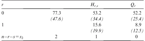
Tables 5a and b present the results from the Hr,s
[image:10.595.305.545.89.239.2]statistic. The numbers in italic are critical values at 95% quantiles. In the case of the 3-variables system (Table 5a), we found s2=1 and consequently s1=1. The seven largest modules of the companion matrix
Table 3a
Decomposing the systems into I(0), I(1) and I(2) spaces; Case 1
ˆ
b0;1 bˆ0;2 bˆ1 kˆ1 bˆt1 bˆt2
temp 1.000 1.000 1.000 79.039 3.921 5.698
rfsun 0.078 4.639 1.638 26.868 3.006 1.937
rfco2 0.792 2.161 7.303 35.985 9.647 2.594 rfch4 0.928 5.565 22.491 21.236 2.074 1.531 rfn2o 36.398 2.774 96.030 1.872 0.258 0.135 trend 0.015 0.004 0.050
ˆ
a0;1 aˆ0;2 aˆ1 aˆt1 aˆt2
temp 0.466 0.067 0.191 0.000 0.001
rfsun 0.034 0.096 0.014 0.001 0.002
rfco2 0.015 0.010 0.005 0.007 0.007
rfch4 0.003 0.002 0.002 0.011 0.095
rfn2o 0.000 0.002 0.000 0.009 0.125
Yt¼ ðtempt;rfsunt;rfco2t;rfch4t;rfn2otÞ#.
Table 3b
Decomposing the systems into I(0), I(1) and I(2) spaces; Case 2
ˆ
b0 bˆ1;1 kˆ1 bˆ1;2 kˆ2 bˆt2;1 bˆt2;2
temp 1 1 17.424 1 20.510 8.404 5.473
rfsun 5.931 0.238 32.565 0.959 3.306 7.540 0.954
rfco2 3.127 5.878 96.770 1.648 28.565 9.968 3.149 rfch4 6.308 12.513 22.507 7.305 8.875 0.838 1.444 rfn2o 16.920 88.710 2.954 14.819 0.401 0.617 0.054
trend 0.003 0.049 0.007
ˆ
a0 aˆ1;1 aˆ1;2 aˆt2;1 aˆt2;2
temp 0.100 0.048 0.646 0.0001 0.002
rfsun 0.075 0.002 0.031 0.001 0.007
rfco2 0.009 0.002 0.017 0.018 0.050
rfch4 0.002 0.000 0.005 0.000 0.139
rfn2o 0.000 0.000 0.000 0.065 0.048
corresponding to the unrestricted VAR are: 0.9942, 0.9297, 0.8402, 0.8402, 0.7796, 0.6543, 0.6543. It seems there are two roots close to the unit circle. Whenr=1 is imposed, the seven largest modules are: 1.000, 1.000, 0.9546, 0.8494, 0.8494, 0.6844, 0.6844. We have two unit roots as the results of restrictionr=1. However, there is another root 0.9546 very close to the unit circle, and this indicates the presence of I(2) trends. Therefore, accord-ing to the results of the eigenvalues of the companion matrix, the total number of unit roots iss1C2s2=3. This is in agreement with the results of the statistic Hr,s.
Because we have the evidence that solar irradiance and temperature are both I(1) variables from univariate tests, it seems that carbon dioxide is the one responsible for the existence of the I(2) trend.
For the system with 2 variables (Table 5b), the results indicate s2=1, therefore, s1=0. In this case, the existence of one I(2) trend is difficult to accept since our preliminary results (see the last sub-section) indicate that there are two explosive roots which should be attributed to the two variables in the 2-variable system. The five largest modules of the companion matrix from the unrestricted VAR are: 1.0393, 1.0393, 0.8374, 0.6901, 0.6901. When r=1 is imposed, the eigenvalues are: 1.029, 1.029, 1.000, 0.714, 0.714. We have one unit root corresponding to the restriction of r=1 and two explosive roots. Others are not close to the unit circle. This information indicates that there is no I(2) trend in this system, whereas it seems to verify that explosive roots mimic the behavior of I(2) trends, as reported by
Haldrup and Lildholdt (2002). Therefore in this case we conclude withr=1,s1=1 and s2=0.
Table 6 shows the estimates of ˆb1;kˆ1;aˆ1;bˆt1;bˆt2;
ˆ
at1 and ˆa12.18 Each year the temperature series
cor-rects 12.6% the disequilibria in the dynamic long-run
steady-state relation ( polynomial cointegration). It is interesting to observe that the I(1) trend is driven by temperature and radiative forcing of solar irradiance but not by radiative forcing of carbon dioxide. However, the I(2) trend is completely driven by this greenhouse gas. The magnitude of the estimates of ˆbt1 tells us that the
I(1) trend affects significantly all variables in the system, with the major effect on temperature series. Because this I(1) trend is driven by the temperature series itself and for the radiative forcing of solar irradiance, the esti-mates of ˆbt1 indicate that this trend corresponds to
‘inertial’ (or persistent) factors (temperature itself) and natural factors (radiative forcing of solar irradiance). In the case of the magnitudes of ˆbt2, the effects are also
appreciated on temperature series. This I(2) trend could correspond to the human factors, that is, the greenhouse gases effects, in this case represented by radiative forcing of carbon dioxide.
[image:11.595.52.290.92.150.2]The cointegration relation detected in the 2-variable system indicates a relationship between radiative for-cing of methane and nitrous dioxide. We introduce this relation (together with the polynomial cointegration relation found in the 3-variable system) in the error correction model to calculate the response of the temperature series to these steady-state relations.19The results indicate that temperature series responds 50.18% to the static long-run relation between radiative forcing of methane and nitrous. These results are in agreement with those results found in the last sub-section.
Table 4a
Testing for cointegrating ranks
H0 lmax Trace lmax90%
critical values
Trace 90% critical values
r=0 36.1 54.5 23.1 39.1
r=1 14.7 18.4 16.9 23.0
r=2 3.7 3.7 10.5 10.6
[image:11.595.311.555.223.292.2]Yt¼ ðtempt;rfsun;rfco2tÞ#.
Table 4b
Testing for cointegrating ranks
H0 lmax Trace lmax90%
critical values
Trace 90% critical values
r=0 43.3 52.2 16.9 23.0
r=1 8.9 8.9 10.5 10.6
Yt¼ ðrfch4t;rfn2otÞ#.
Table 5a
Testing for integration indices
r Hr,s Qr
0 213.5 114.9 58.0 54.5
(86.7) (68.2) (53.2) (42.7)
1 102.0 21.6 18.4
(47.6) (34.4) (25.4)
2 6.4 3.7
(19.9) (12.5)
nrs=s2 3 2 1 0
Yt¼ ðtempt;rfsun;rfco2tÞ#.
Table 5b
Testing for integration indices
r Hr,s Qr
0 77.3 53.2 52.2
(47.6) (34.4) (25.4)
1 15.6 8.9
(19.9) (12.5)
nrs=s2 2 1 0
Yt¼ ðrfch4t;rfn2otÞ#.
18
There is no similar estimates in the case of the 2-system variables because there are not I(2) trends.
19For each one of the cases presented, we estimated the respective
FromTable 6, we found thatDT2x¼2:15(C, which
is in agreement with past literature, seeKaufmann and Stern (2002).
4.4. The third case
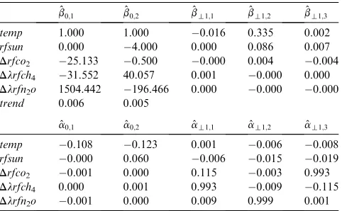
Another alternative is to transform the variables in such a way that an I(1) framework can be performed. Based on the results outlined before, temperature series and radiative forcing of solar irradiance are I(1) pro-cesses. Hence they enter the new system in levels. Radiative forcing of carbon dioxide is most likely an I(2) process and then enters the system in the first differences (Dr f co2). For the case of radiative forcing of methane
and nitrous dioxide, we found evidence of explosiveness. Therefore we apply filterDlðDlyt¼ytlyt1Þto these
[image:12.595.304.545.89.222.2]variables with l=1.029. In summary, our 5-variables system is now composed ofyt¼ ftempt;r f sunt;Drfco2t; Dlrfch4t;Dlrfn2otg:
Table 7 presents the results from the application of the Trace and lmax statistics and it suggests r=2. In
order to be sure that our system does not contain I(2) trends,Table 8presents the results of theHr,sstatistics.
The results confirm our claim. Therefore the integration indices are r=2 and s1=nr=3. The eight largest modules of the companion matrix for the unrestricted VAR are: 0.9581, 0.9581, 0.923, 0.923, 0.861, 0.861, 0.848, 0.848. In the case of the restricted VAR (r=2), these modules are: 1.000, 1.000, 1.000, 0.890, 0.890, 0.858, 0.858, 0.838. We have three unit roots corre-sponding to the restriction ofr=2 and no other roots
[image:12.595.41.284.90.199.2]close to the unit circle.20 The results seem to confirm that the total number of unit roots is three implying that there are not I(2) trends.
Table 9 presents the estimates of the two cointegra-ting vectors, the loadings values and the I(1) trends. The null hypothesis for the long-run exclusion of solar irradiance in the first steady-state relation and the imposition of a coefficient of0.5 associated to carbon dioxide was not rejected with ac2
ð1Þ¼2:75
correspond-ing to a P-value of 0.10. The long-run exclusion of the time trend was always strongly rejected.
The estimates of the adjustment parameters show that temperature series is error correcting 10.8% and 12.3% each year. The first I(1) trend is driven by three greenhouse gases with a larger weight on radiative forcing of methane. The second I(1) trend is almost completely driven by radiative forcing of nitrous dioxide but with a small participation of radiative forcing of solar irradiance. The last I(1) trend is driven by two greenhouse gases with a larger weight on radiative
Table 6
Decomposing the systems into I(0), I(1) and I(2) spaces
ˆ
b1 kˆ1 bˆt1 bˆt2
temp 1.000 0.819 10.505 2.606
rfsun 3.341 0.085 4.396 0.269
rfco2 0.500 1.073 8.366 3.414
trend 0.006
ˆ
a1 aˆt1 aˆt2
temp 0.126 0.046 0.000
rfsun 0.069 0.085 0.001
rfco2 0.001 0.001 0.096
[image:12.595.306.547.271.420.2]Yt¼ ðtempt;rfsunt;rfco2tÞ#.
Table 7
Testing for cointegrating ranks
H0 lmax Trace lmax90%
critical values
Trace 90% critical values
r=0 57.2 131.4 34.8 82.7
r=1 42.4 74.3 29.1 59.0
r=2 17.0 31.9 23.1 39.1
r=3 9.6 14.8 16.9 23.0
r=4 5.2 5.2 10.5 10.6
Yt¼ ðtempt;rfsunt;Drfco2t;Dlrfch4t;Dlrfn2otÞ#.
Table 8
Testing for integration indices
r Hr,s Qr
0 506.9 384.1 302.3 224.8 163.1 131.4
(198.2) (167.9) (142.2) (119.8) (101.5) (87.2)
1 373.1 254.4 173.4 106.9 74.3
(137.0) (113.0) (92.2) (75.3) (62.8)
2 239.8 155.3 75.8 31.9
(86.7) (68.2) (53.2) (42.7)
3 130.6 52.3 14.8
(47.6) (34.4) (25.4)
4 23.2 5.2
(19.9) (12.5)
nrs=s2 5 4 3 2 1 0
Yt¼ ðtempt;rfsunt;Drfco2t;Dlrfch4t;Dlrfn2otÞ#.
Table 9
Decomposing the systems into I(0), I(1) and I(2) spaces
ˆ
b0;1 bˆ0;2 bˆt1;1 bˆt1;2 bˆt1;3
temp 1.000 1.000 0.016 0.335 0.002
rfsun 0.000 4.000 0.000 0.086 0.007
Drfco2 25.133 0.500 0.000 0.004 0.004
Dlrfch4 31.552 40.057 0.001 0.000 0.000 Dlrfn2o 1504.442 196.466 0.000 0.000 0.000
trend 0.006 0.005
ˆ
a0;1 aˆ0;2 aˆt1;1 aˆt1;2 aˆt1;3
temp 0.108 0.123 0.001 0.006 0.008
rfsun 0.000 0.060 0.006 0.015 0.019
Drfco2 0.001 0.000 0.115 0.003 0.993 Dlrfch4 0.000 0.001 0.993 0.009 0.115 Dlrfn2o 0.001 0.000 0.009 0.999 0.001
Yt¼ ðtempt;rfsunt;Drfco2t;Dlrfch4t;Dlrfn2otÞ#.
20In economics, some researchers consider that an eigenvalue of
[image:12.595.42.281.646.725.2]forcing carbon dioxide and again, a small participation of radiative forcing of solar irradiance.
5. Conclusions
This paper applies multivariate I(1) and I(2) tools to identify for the existence and the number of long-run steady-state relations between temperature series and radiative forcing of solar radiance and a set of three greenhouse gases. One of the results indicate that temperature and radiative forcing of solar irradiance series appear to be I(1) processes, radiative forcing of carbon dioxide is an I(2) process, and radiative forcing of methane and nitrous dioxide seem to contain explosive roots. In most variables (temperature, radia-tive forcing of solar irradiance and carbon dioxide), our results confirm previous evidence in the literature.
Given the complex structure and properties of the time series, we analyzed three alternative cases. In the first case, a 5-variable system is considered. The second case consisted of variables with I(1) and I(2) characteristics and the ones with explosive behavior separately. The last system considers a transformation of the variables in such a way that the I(1) framework can be used. Overall, all systems show that temperature series is error correcting the disequilibria towards the static steady-state or dynamic steady-state relations. The degree of adjustment of the temperature depends on which cointegrating relations is considered but it goes from 5% to 65%. The higher rates of adjustment are comparable to the results found by Stern and Kaufmann (2000). In some cases, however, temperature series is not error correcting for the long-run disequilibria. It means that there is nothing in the system (the earth and its components) that allows for correcting these disequilibria. On the other hand, the higher rates of adjustment respect to other disequilibria could suggest abrupt changes in temperature in order to correct for these disequilibria.
Another interesting result is the composition of the I(1) and I(2) trends. According to our results, both trends are essentially composed by a linear combination of greenhouse gases that are affecting the temperature series strongly. In an specific case, we find that the I(1) trend is driven by temperature and radiative forcing of solar irradiance, whereas the I(2) trend is driven by a linear combination of the three greenhouse gases or exclusively by the radiative forcing of carbon dioxide. The first component could be associated to inertial and/ or natural factors. In the case of the second component, it could be related to human factors.
Finally, we find that the equilibrium temperature change for a doubling of carbon dioxide is between 2.15 and 3.4(C, which is agreement with previous literature
and the report of the IPCC (2001) using 15 different general circulation models.
Acknowledgements
An earlier version of this paper has benefited from useful comments from the participants to the 35th Annual Conference of the Canadian Economic Associ-ation, Calgary, 2001. We thank constructive comments from two referees and the Editor. The writing of this paper was finished while G.R. was visiting the School of Economics of the University of New South Wales, Australia, and he thanks particularly Garry Barret. Financial support from the Faculty of Social Sciences is acknowledged.
References
Bloomfield, P., 1992. Trends in global temperature. Climatic Change 21, 1e16.
Bloomfield, P., Nychka, D., 1992. Climate spectra and detecting climate change. Climatic Change 21, 275e287.
Dickey, D.A., Fuller, W.A., 1979. Distribution of the estimators for autoregressive time series with a unit root. Journal of the American Statistical Association 74, 427e431.
Dickey, D.A., Pantula, S.G., 1987. Determining the order of differ-encing in autoregressive process. Journal of Business and Economic Statistics 5, 455e461.
Doornik, D.A., Hendry, D.F., 2001. Modelling Dynamic Systems Using PcGive 10.0, vol. II. Timberlake Consultants, UK. Elliott, G., Rothenberg, T., Stock, J.H., 1996. Efficient tests for an
autoregressive unit root. Econometrica 64, 813e839.
Fiess, N., MacDonald, R., 2001. The instability of the money demand function: an I(2) interpretation. Oxford Bulletin of Economics and Statistics 63 (4), 475e495.
Fomby, T., Vogelsang, T., 2002. Application of size robust trend analysis to global warming temperature series. Journal of Climate 15, 117e123.
Galbraith, J.W., Green, C., 1993. Inference about trend in global temperature data. Climatic Change 22, 209e221.
Haldrup, N., 1999. A review of the econometric analysis of I(2) variables. In: Oxley, L., McAleer, M. (Eds.), Practical Issues in Cointegration Analysis. Blackwell, Oxford.
Haldrup, N., Lildholdt, P., 2002. On the robustness of unit root tests in the presence of double unit roots. Journal of Time Series Analysis 23 (2), 155e171.
Hansen, H., Juselius, K., 1995. CATS in RATS, Manual to Cointegration Analysis of Time Series. Estima, Evanston, IL. Harvey, A.C., 1989. Forecasting, Structural Time Series Models, and
the Kalman Filter. Cambridge University Press.
Hasza, D.P., Fuller, W.A., 1979. Estimation of autoregressive processes with unit roots. Annals of Statistics 7, 1106e1120. Holtemo¨ller, O., 2002. Money and Prices: An I(2) Analysis for the
Euro Area. Working Paper. Humboldt-Universita¨t, Berlin. IPCC (Intergovernmental Panel on Climate Change). 2001. In:
Houghton, J.T., Ding, Y., Griggs, D.J. (Eds.), Climate Change 2001: the Intergovernmental Panel on Climate Change Scientific Assessment. Cambridge University Press, Cambridge, UK, New York, NY, USA, pp. 358.
Johansen, S., 1988. Statistical analysis of cointegration vectors. Journal of Economic Dynamics and Control 12, 231e254. Johansen, S., 1992. A representation of vector autoregressive process
of order 2. Econometric Theory 8, 188e202.
Johansen, S., 1995b. Likelihood-Based Inference in Cointegrated Vector Autoregressive Models. Oxford University Press, Oxford. Johansen, S., Juselius, K., 1992. Testing structural hypothesis in
a multivariate cointegration analysis of the PPP and the UIP for UK. Journal of Econometrics 53, 211e244.
Johansen, S., Juselius, K., 1994. Identification of the long-run and the short-run structure. An application to the ISLM Model. Journal of Econometrics 63, 7e36.
Juselius, K., 1999. Price convergence in the medium and long run: an I(2) analysis of six price indices. In: Engle, R.F., White, H. (Eds.), Cointegration, Causality and Forecasting (A Festschrift in Honour of Clive W.J. Granger). Oxford University Press, New York. Juselius, K., 2003. Inflation, money growth, and I(2) analysis.
Unpublished manuscript.
Kaufmann, A., Stern, D.I., 1997. Evidence for human influence on climate from hemispheric temperature relations. Nature 388, 39e44. Kaufmann, A., Stern, D.I., 2002. Cointegration analysis of hemi-spheric temperature relations. Journal of Geophysical Research 107 (D2), 10.1029/2000JD000174.
Kelly, D.L., 2000. Unit Roots in the Climate: Is the Recent Warming Due to Persistent Shocks? Working Paper. Department of Eco-nomics, University of Miami.
Kuo, C., Lindberg, C., Thompson, D.J., 1990. Coherence established between atmospheric carbon dioxide and global temperature. Nature 388, 39e44.
Kongsted, H.C., 2003. An I(2) Cointegration Analysis of Small-Country Import Price Determination. Institute of Economics, University of Copenhagen.
Lean, J., Beer, J., Bradley, R., 1995. Reconstruction of solar irradiance since 1610: implications for climate change. Geophysical Research Letters 22, 3195e3198.
Lenten, L.J.A., Moosa, I.A., 2003. An empirical investigation into long-term climate change in Australia. Environmental Modelling & Software 18, 59e70.
Nielsen, B., 2001. The Asymptotic distribution of unit root tests of unstable autoregressive processes. Econometrica 69, 211e219. Nielsen, B., 2002. Cointegration Analysis of Explosive Processes.
Discussion Paper. Nuffield College, Oxford.
Paruolo, P., 1996. On the determination of integration indices in I(2) systems. Journal of Econometrics 72, 313e356.
Paruolo, P., Rahbek, A., 1999. Weak exogeneity in I(2) VAR systems. Journal of Econometrics 93, 281e308.
Phillips, P.C.B., Perron, P., 1988. Testing for a unit root in time series regression. Biometrika 75, 335e346.
Rahbek, A., Kongsted, H.C., Jorgensen, C., 1999. Trend stationarity in the I(2) cointegration model. Journal of Econometrics 90, 265e289.
Richards, G.R., 1993. Change in global temperature: a statistical analysis. Journal of Climate 6, 546e559.
Said, E.S., Dickey, D.A., 1984. Testing for unit roots in autoregressive-moving average models of unknown order. Biometrika 71, 599e607.
Santer, B.D., Taylor, K.E., Wigley, T.M.L., Johns, T.C., Jones, P.D., Karoly, D.J., Mitchell, J.F.N., Oort, A.H., Penner, J.E., Ram-aswamy, V., Schwartzkopf, M.D., Stouffer, R.J., Tett, S., 1996. A search for human influences on the thermal structure of the atmosphere. Nature 382, 39e46.
Schmidt, P., Phillips, P.C.B., 1992. LM tests for a unit root in the presence of deterministic trends. Oxford Bulletin of Economics and Statistics 54, 257e287.
Scho¨nwiese, C.-D., 1994. Analysis and prediction of global climate temperature change based on multiforced observational statistics. Environmental Pollution 83, 149e154.
Stern, D.I., Kaufmann, R.K., 1997. Time Series Properties of Global Climate Variables: Detection and Attribution of Climate Change. Working Paper in Ecological Economics, 9702. Center for Resource and Environmental Studies, Australian National Uni-versity.
Stern, D.I., Kaufmann, R.K., 1999. Econometric analysis of global climate change. Environmental Modelling & Software 14, 597e605.
Stern, D.I., Kaufmann, R.K., 2000. Detecting a global warming signal in hemispheric temperature series: a structural time series analysis. Climatic Change 47, 411e438.
Stock, J.H., Watson, M.W., 1998. Testing for common trends. Journal of the American Statistical Association 83, 1097e1107.
Tol, R.S., DS, J., 1994. Greenhouse statistics-time series analysis: part II. Theoretical and Applied Climatology 49, 63e74.
Tol, R.S., de Vos, A.F., 1998. A Bayesian statistical analysis of the enhanced greenhouse effect. Climatic Change 38, 87e112. Thomson, D.J., 1995. The seasons, global temperature, and precession.
Science 268, 59e68.
Thomson, D.J., 1997. Dependence of global temperatures on atmospheric CO2and solar irradiance. Proceedings of the National
Academy of Sciences USA 94, 8370e8377.
Vostroknutova, E., 2003. Shock Therapy? An I(2) Cointegration Analysis of the Russian Stabilization. EUI Working Paper ECO, No. 2003/16. Department of Economics, European University Institute.
Woodward, W.A., Gray, H.L., 1993. Global warming and the problem of testing for trend in time series data. Journal of Climate 6, 953e962.