Decoupling Multivariable Processes using Partial Least
Squares for Decentralized Control
Seshu Kumar Damarla
Department of Chemical Engineering National Institute of Technology Rourkela, IndiaMadhusree Kundu
Department of Chemical Engineering National Institute of Technology Rourkela, IndiaABSTRACT
Multivariable control systems suffer very much from unwanted interactions among control loops. Change in setpoint of one variable may cause other variables to deviate from their respective steady states because of couplings between unpaired variables. Due to unreliability problems, conventional decouplers are not appropriate for higher order processes. This paper proposes Partial Least Squares (PLS), multivariate statistical process control technique (MVSPC), based decoupling strategy to attain satisfactory performance and consistent product quality in spite of disturbances. The proposed scheme was applied on conventional and heat integrated distillation processes. The results have shown the reliability and robustness of Partial Least Squares based decouplers over conventional decouplers.
General Terms
Process Identification & control, Statistical Process Control
Keywords
PLS, multivariable interactions, decoupling
1.
INTRODUCTION
Interactions between control loops can have significant impact on final product quality. The presence of redundant interactions and effect of unknown disturbances complicated the control of nonlinear and dynamic multivariable processes. Hence avoiding unnecessary loop interactions in multi-loop control systems is vital for safe and desired operation. In multi input-multi output (MIMO) systems, input and output variables can be paired by using relative gain array [1]. Gangnepaln & Seborg (1982) presented a new measure of interactions based on average dynamic gains for determination of best pairing [2]. Conventional decouplers have been in use for elimination of adverse effects on exact pairing of two input-two output (2×2) systems [3-8]. Wade (1997) proposed an inverted decoupler that produces process input signals by combining one controller output with other input signals [9]. Gagnon et al. (1998) provided guidelines and summary of advantages & limitations of decoupling methods for 2×2 systems [10]. Shiu & Hwang (1998) presented sequential tuning of MIMO control system based on ultimate frequency that ranks each loop from fast to slow [11]. Gjosaeter & Foss (1997) argued that discarding the use of decouplers for ill conditioned process is not essential [12]. Chien et al. (2000) proposed one way decoupling by assuming the open loop process dynamics of heterogeneous azeotropic distillation as integrator plus time delay [13]. Artificial neural network based decoupling approach has been applied by Chai et al. (2011) to ball mill coal pulverizing systems in heat power plant [14]. On the other hand conventional decouplers have become ineffective in case of non-minimum phase
Partial Least Squares (PLS) finds latent variables that are associated with the maximum variation in process data and provides diagonal pairings of latent variables as strong as possible. PLS facilitates in identifying an empirical model from plant data without making any assumptions. First proposed by Wold (1966) PLS has been successfully applied in diverse fields including process monitoring, identification and control and it deals with noisy and highly correlated data, quite often, only with a limited number of observations available [15]. A tutorial description along with some examples on the PLS model was provided by Geladi Kowalaski (1986) [16]. When dealing with nonlinear systems, the underlying nonlinear relationship between predictor variables (X) and response variables (Y)can be approximated by quadratic PLS (QPLS) or splines. Sometimes it may not function well when the non-linearities cannot be described by quadratic relationship. Artificial Neural Networks (ANN) can be used to find inner relation to handle nonlinearities [17-23]. This approach employs the neural network as inner model keeping the outer mapping framework as linear PLS algorithm. The conventional PLS is suitable for modeling time independent or steady state processes. Kaspar and Ray (1993) developed dynamic extension of the PLS models by filtering the process inputs and subsequent application of the standard PLS algorithm and demonstrated their approach for identification & control problem using linear models [24]. Lakshminarayanan (1997) proposed the ARX/Hammerstein model as the modified PLS inner relation and used successfully in identifying dynamic models and proposition of PLS based feed forward and feedback controllers [25]. Damarla & Kundu (2011) proposed PLS based artificial neural network scheme for identification and control of distillation process [26]. Kaspar & Ray, Lakshminarayanan and Damarla & Kundu have proposed closed loop control system which uses pre and post compensators acquired from loadings of PLS model for mapping outputs and inputs into physical variables.
data, SISO process models are identified from corresponding pair of input-output scores and feedback control system is designed using identified process model. The rest of the paper is organized as follows. Section 2 presents theory of PLS. PLS based decoupled control system is described in section 3. Conventional and heat integrated distillation processes are considered in section 4 & 5, respectively, to evaluate the performance of the proposed decoupling scheme. Finally, conclusive remarks are made.
2.
PARTIAL LEAST SQUARES
Pseudo random binary sequence (PRBS) of inputs can excite multivariable process for identification. X and Y matrices (Input - output) are scaled in the following way before they are processed by PLS algorithm.
1
XSX
X and Y YSY1 (1)
Where
n
X
S
X
S
X
S
X
S
0
0
0
0
0
2
0
0
0
1
and
n
Y
S
Y
S
Y
S
Y
S
0
0
0
0
0
2
0
0
0
1
X
S and SYare scaled matrices. The basic idea of PLS is to develop a model by relating the scores of X and Y data. PLS model consists of outer relations that decompose X & Y data individually as a summation of product of score vector and loading vector and inner relations that links X data to Y data through their scores. The outer relationship for the input matrix and output matrix can be written as
E
T
TP
E
T
n
p
n
t
T
p
t
T
p
t
X
1
1
2
2
...
(2)F T UQ F T n q n u T q u T q u
Y 1 1 2 2 ..
(3) Where T and Urepresent the matrices of scores of X and Y while Pand Qrepresent the loading matrices for X and Y . If all the components of X and Y are described, the errors E& F become zero.
The inner model that relates X to Y is the relation between the scores T & U.
TB
U (4)
Where B is the regression matrix. The response Y can now be expressed as:
F TBQ
Y T (5) To determine the dominant direction of projection of X and Y data, the maximization of covariance within X and Y is used as a criterion. The first set of loading vectors p1 and q1 represent the dominant direction obtained by maximization of covariance within X and Y . Projection of X data on p1 and Y data on q1 resulted in the first set of score vectors t1 and u1 , hence the establishment of outer relation. The matrices X and Y can now be related through their respective scores, which is called the inner model, representing a linear regression between t1 andu1: uˆ1t1b1. The calculation of first two dimensions is shown in Fig. 1. The residuals are calculated at this stage is given by the following equations.
1 1
1 X t p
E (6)
1 1 1 1 1
1 Y uq Y tbq
F (7) The procedure for determination of the scores and loading vectors is continued by using newly computed residuals till they become small enough or the number of PLS dimensions required is reached. In practice, number of PLS dimensions is calculated by percentage of variance explained and cross validation. The irrelevant directions originating from noise and redundancy are left as EandF . PLS relates one pair of latent variables (t1u1) at each stage, thereby making path for identification of input-output pairings
y1u1,y2u2,....ynun
in lower dimensions
t1u1,t2u2,....tnauna
thus eliminates undesirable interactions
y1u2,y2u1,etc.
. Therefore, MIMO system can be decomposed into series of single input single output (SISO) systems.3.
CLOSED LOOP CONTROL SYSTEM
Fig 1: If necessary, the images can be extended both columns
4.
EXAMPLE 1: WOOD-BERRY
DISTILLATION COLUMN
Wood-Berry distillation column, which is used for separation of methanol-water mixture, has been adapted in this work to assess the proposed PLS decoupling scheme [28]. The control variables are compositions of methanol in top and bottom products. Reflux rate and reboiler steam flow rate can serve as manipulate variables to control top and bottom product compositions. Equation (8) expresses relation between outputs and inputs (manipulated and disturbance variables (feed flow rate & feed composition)). The control and manipulate variables were paired (
y
1
u
1;
y
2
u
2) according to relative gain array results bestowed in Table 1. The conventional simplified decouplers shown in equation (9) were determined to eliminate interactions between unpaired variables. Two PID controllers were designed based on minimum overshoot and offset free response criteria. The values of tuning parameters of two controllers can be found in Table 2.Fig 2: Decoupled multivariable control system.
) ( ) ( 1 1 . 12 ) 2 . 9 exp( 14 . 0 1 2 . 13 ) 4 . 3 exp( 9 . 4 1 8 . 22 ) 7 . 7 exp( 22 . 0 1 9 . 14 ) 1 . 8 exp( 8 . 3 ) ( ) ( 1 4 . 14 ) 3 exp( 4 . 19 1 9 . 10 ) 7 exp( 6 . 6 1 21 ) 3 exp( 9 . 18 1 7 . 16 ) exp( 8 . 12 ) ( ) ( 2 1 1 1 2 1 s d s d s s s s s s s s s u s u s s s s s s s s s y s y (8)
1 21 ) 2 exp( 4766 . 1 659 . 2412
s s s d
1 9 . 10 ) 4 exp( 3438 . 0 95072 . 4 21 s s sd (9)
[image:3.595.313.543.340.590.2] 07281 . 0 ) 07 . 3 exp( 2036 . 0 0 0 06509 . 0 ) 02 . 3 exp( 1969 . 0 s s s s GPLS (10)
Table 1: RGA analysis for Example 1
Manipulated Inputs
Ou
tp
u
ts
u1 u2
y1 2.0094 -1.0094
y2 -1.0094 2.0094
u
-
Gc PLS Model
d
+ + Y
+ nn g g g 0 0 0 0 0 0 0 0 0 0 0 0 22 11 Cn C C g g g 0 0 0 0 0 0 0 0 0 0 0 0 2 1 r X Y
-
+ Error F2
Higher Dimension 2 ˆ u 1
ˆ
u
2 ˆ y 1 ˆ y q1-
-
+ +-
+ p2 t2 u2 q2 t1 u1 p1Error E2
Error E1
Error F1
PLS Outer model 1 Inner model 1 × PLS Outer model 2 Inner model 2
[image:3.595.64.538.340.726.2]Table 2: PID controller parameters for Example 1
PID controller parameters Proporti
onal
Integral Derivative
P
airi
n
g
Loop 1 u1-y1 -1.4821 -0.05608 --0.6269
[image:4.595.318.561.142.346.2]Loop 2 u2-y2 -0.09 -0.005 -0.09 The form of PID controller used in this work is PID=P+I/ s + D s
Table 3: PLS based PID controllers
PID controller parameters
Proportional Integral Derivative
P
airi
n
g
Loop 1 u1-y1 -0.1 -0.012 -0.01
Loop 2 u2-y2 -0.09 -0.011 -0.001
The form of PID controller used in this work is PID=P+I/s+Ds
Database required for PLS has been generated by simulating the distillation process with pseudo random binary signals. Signal to noise ratio was set to 10 by adding white noise to process data. Matlab System Identification (GUI) tool was used to determine the inner relations of
X
andY
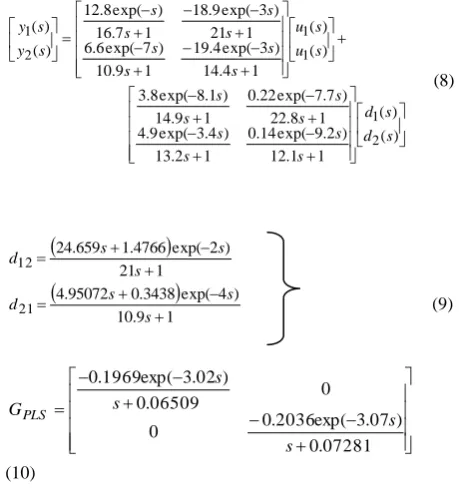
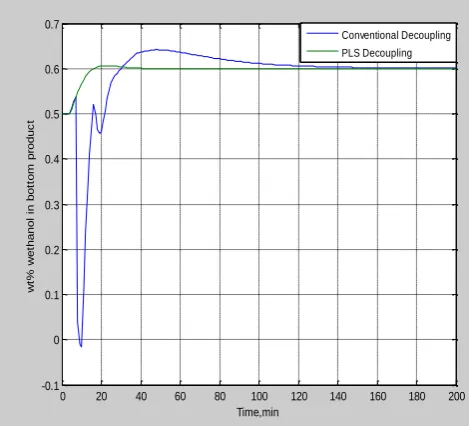
as linear process models. Equation (10) bestows the identified linear process models in transfer function matrix. Two PID controllers were designed using identified linear process models on the basis of minimum overshoot and offset free response criteria. Table 3 furnishes the values of tuning parameters of PID controllers. Simultaneous step setpoint changes of magnitude 2 & 0.1 were made at t=1th sampling instant in top (from 96 to 98) and bottom product (from 0.5 to 0.6) compositions, respectively. The conventional as well as PLS based decoupled control systems were simulated over 3.33 hours with sampling time of 1 minute. Figs. 3 and 4 show comparison of responses of methanol in top and bottom product acquired from two decoupling strategies. In bringing top product and bottom compositions to new setpoints, PLS decoupled control system exhibited good performance than conventional system. A unit step change was made in feed composition to check the robustness of the proposed approach in presence of disturbance. As depicted in figs 5 and 6, bothdecoupling approaches were successfully rejected disturbance’s impact on process but settling times are relatively large in conventional system.
Fig 3: Comparison of responses of conventional and PLS decoupling strategies for setpoint change in top product
from 96 to 98
Fig 4: Comparison of responses of conventional and PLS decoupling strategies for setpoint change in bottom
product from 0.5 to 0.6
0 20 40 60 80 100 120 140 160 180 200 96
96.5 97 97.5 98 98.5
Time,min
w
t%
m
e
th
a
n
o
l
in
t
o
p
p
ro
d
u
c
t
Conventional Decoupling PLS Decoupling
0 20 40 60 80 100 120 140 160 180 200 -0.1
0 0.1 0.2 0.3 0.4 0.5 0.6 0.7
Time,min
w
t%
w
e
th
a
n
o
l
in
b
o
tt
o
m
p
ro
d
u
c
t
[image:4.595.319.554.433.646.2]Fig 5: Comparison of responses of top product for unit step change in feed composition
Table 4: RGA analysis for Example 2
Manipulated Inputs
Ou
tp
u
ts
u1 u2 u3 u4
y1 2.098 -0.998 0 -0.1 y2 -1.039 1.332 0 0.707
y3 0.41 -0.563 1.514 0.008
y4 -0.100 1.259 -0.514 0.385
Fig 6: Comparison of responses of bottom product for unit
5.
EXAMPLE 2: HEAT INTEGRATED
DISTILLATION COLUMN
Along with wood-Berry Distillation process, heat integrated distillation process, which produces low purity products (96 mol% methanol overhead and 4 mol% methanol bottoms composition), has taken from literature [29]. Feed split configuration was selected among four configurations since it is difficult to control. Relation between controlled variables (overhead and bottoms compositions in both high and low pressure columns) and manipulated variables (reflux flow rate in high pressure column, reboiler heat input to high pressure column, reflux flow rate in low pressure column and feed split) is provided by equation (11) and equation (12) describes relation between controlled variables and disturbance variable (feed composition). The diagonal input-output pairings are possible as per RGA results conferred in Table 4. Table 5 gives the values of parameters of four conventional PID controllers designed based on dynamic performance criteria. The presence of time delays in the process transfer function made simplified decouplers practically unrealizable, therefore static decoupling matrices given by equation (13) were computed using least squares technique.
1 20 ) 6 . 0 exp( 92 . 6 ) 1 )( 1 5 . 18 ( ) 9 . 0 exp( 2 . 12 ) 1 )( 1 20 ( 5 . 34 ) 1 )( 1 21 ( ) exp( 82 . 1 ) 1 3 )( 1 6 . 11 )( 1 21 ( ) 1 7 . 78 ( 042 . 0 ) 1 4 )( 1 13 ( 6 . 3 ) 1 4 )( 1 13 ( 66 . 4 ) 1 4 )( 1 5 . 17 ( ) 2 . 1 exp( 22 . 0 ) 1 20 ( ) 3 . 0 exp( 2 . 9 0 ) 1 )( 1 21 ( 41 ) 1 5 . 0 )( 1 17 ( ) 9 . 0 exp( 3 . 17 ) 1 2 )( 1 7 . 25 ( 35 . 0 0 ) 1 4 )( 1 16 ( 4 . 7 ) 1 4 )( 1 14 ( 45 . 4 s s s s s s s s s s s s s s s s s s s s s s s s s s s s s s s s s s L F H F L R RH Q H R BL X DL X BH X DH X (11)
Zs s s s s s s s s s s s X X X X BL DL BH DH ) 1 2 )( 1 25 ( ) 6 . 0 exp( 61 . 16 ) 1 2 )( 1 6 . 15 ( ) 5 exp( 75 . 0 ) 1 )( 1 25 ( ) 3 . 0 exp( 7 . 19 ) 1 2 )( 1 25 ( ) 5 . 4 exp( 02 . 1 2 2 (12) 3839 . 0 5813 . 0 3414 . 0 41 31 21 d d d ; 7416 . 2 5418 . 0 7142 . 3 42 32 12 d d d 5071 . 0 3807 . 0 6303 . 0 43 23 13 d d d ; 2820 . 0 1307 . 0 8062 . 0 34 24 14 d d d (13) 03877 . 0 1404 . 0 0 0 0 0 01065 . 0 5357 . 0 07719 . 0 0 0 0 0 009328 . 0 3968 . 0 06782 . 0 0 0 0 0 009217 . 0 2925 . 0 0477 . 0 2 2 2 s s s s s s s G (14)
0 20 40 60 80 100 120 140 160 180 200 96 96.2 96.4 96.6 96.8 97 97.2 97.4 97.6 97.8 Time,min w t% m e th a n o l in t o p p ro d u c t Conventional Decoupling PLS Decoupling
Table 5: PID controller parameters for Example 2
PID controller parameters
Loop Proportiona
l
Integral Derivative
P
airi
n
g
1 2 3 4
u1-y1 3.1675 0.0672 3.4031
u2-y2 -0.7948 -0.0231 -0.2753
u3-y3 2.7567 0.12906 3.2123
u4-y4 0.1404 0.009 0.04
The form of PID controller used in this work is PID=P+I/s+Ds
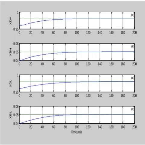
Similarly, process data was collected by exciting heat integrated distillation process with pseudo random binary signals in order to determine SISO process models in latent space. Signal to noise ratio was set to 10. Equation (14) presents process transfer function matrix having inner relation of X and Y on its diagonal. Four number of PLS based PID controllers, values of those are provided in Table 6, were designed to control the overhead and bottoms compositions in both high and low pressure columns. Both decoupled control systems were simulated over 3.33hours with sampling period of 1 minute. Simultaneous step setpoint changes of magnitude 0.02 and 0.01 were made at t=1st instant in overhead (from 0.96 to 0.98) and bottoms (from 0.04 to 0.05) compositions, respectively, in both columns. The static decoupling strategy exhibited worst performance in tracking new setpoints as shown in fig. 7. The overhead and bottoms composition in high pressure column are continuously increasing with time whereas in low pressure column, it is quite opposite. Nonetheless PLS decoupling scheme moved the process to new steady state region which is depicted in fig. 8. Fig. 9 displays influence of unit step change in feed composition on conventionally decoupled control system. The process variables are going away from steady states in high and low pressure columns. As demonstrated in fig. 10, the control system with PLS based decouplers suppressed the effect of disturbance on process and maintained the products at desired values.
Table 6: PLS based PID controllers for Example 2
PID controller parameters
Proportional Integral Derivative
P
airi
n
g
Loop 1 Loop 2 Loop 3 Loop 4
u1-y1 0.1404 0.006 0.04 u2-y2 0.1404 0.004 0.06
u3-y3 0.1404 0.0035 0.04
[image:6.595.49.300.92.240.2]u4-y4 0.1404 0.009 0.04 The form of PID controller used in this work is PID=P+I/s+Ds
Fig 7: Response of conventional decoupled system for setpoint changes in top and bottom product compositions
in both columns.
Fig 8: Response of PLS based decoupled system for setpoint changes in top and bottom product compositions
in both columns.
0 20 40 60 80 100 120 140 160 180 200
0.5 1 1.5
X
D
H
0 20 40 60 80 100 120 140 160 180 200
0 0.2 0.4
XBH
0 20 40 60 80 100 120 140 160 180 200
0.7 0.8 0.9
X
D
L
0 20 40 60 80 100 120 140 160 180 200
-10 0 10
Time,min
XBL
(d) (c) (b) (a)
0 20 40 60 80 100 120 140 160 180 200 0.95
1
X
D
H
0 20 40 60 80 100 120 140 160 180 200 0.04
0.05 0.06
XBH
0 20 40 60 80 100 120 140 160 180 200 0.95
1
X
D
L
0 20 40 60 80 100 120 140 160 180 200 0.04
0.05 0.06
Time,min
XBL
[image:6.595.317.558.380.622.2] [image:6.595.50.295.612.747.2]Fig 9: Response of conventional decoupled control system for unit step change in feed composition.
Fig 10: Response of PLS decoupled control system for unit step change in feed composition.
6.
CONCLUSIONS
By utilizing advantage of PLS i.e. decomposing multivariable regression problems into series of single variable regression problems, undesirable interactions in the conventional and heat integrated distillation processes were eliminated. Once the processes were decoupled perfectly, linear SISO process models were estimated from each pair of input-output scores. PID controllers were designed for both conventional and PLS
overshoot and offset free response criteria. The closed loop control system with PLS based decouplers maintained process variables (example 1) at their respective steady sates in the presence of external influences. In case of higher order process (example 2), the results have proven the necessity of realizable decouplers for elimination of couplings between unpaired variables. The performance of PLS based decoupling strategy is compared with the conventional decoupling approach in two cases and this comparison recommends the application of PLS based decoupling scheme in a wide variety of processes including non-minimum phase process.
7.
REFERENCES
[1] H. B. Edgar, “On a New Measure of Interaction for Multivariable Process Control”, IEEE T. Automat. Contr, Vol. 11 (1), (January, 1966), pp: 133-134.
[2] J-P. Gagnepaln, D. E. Seborg, “Analysis of Process Interactions with Applications to Multiloop Control System Design”, Ind. Eng. Chem. Process Des. Dev., Vol. 21, (1982), pp: 5-11.
[3] W.L. Luyben, “Distillation decoupling”, AIChE J., Vol. 16 (2), (1970), pp: 198-203.
[4] K. V. T. Waller, “Decoupling in distillation”, AIChE J., Vol. 20 (3), (1974), pp: 592-594.
[5] T. J. McAvoy, “Steady-State Decoupling of Distillation Columns”, Ind. Eng. Chem. Fundam., Vol. 18 (3), (1979), pp: 269-273.
[6] K. Weischedel, T. J. McAvoy, “Feasibility of decoupling in conventionally controlled distillation columns”, Ind. Eng. Chem. Fundam., Vol. 19 (4), (1980),pp: 379-384. [7] Y. Arkun, B. Manouslouthakis, A. Palazoglu,
“Robustness analysis of process control systems. A case study of decoupling control in distillation”, Ind. Eng. Chem. Process Des. Dev., Vol. 23 (1), (1984), pp: 93-101.
[8] D. E. Seborg, T. F. Edgar, D. A. Mellichamp, “Process Dynamics & Control”, John Wiley & Sons, New York, 1989.
[9] H. L. Wade, “Inverted decoupling: a neglected technique”, ISA T., Vol. 36 (1), (1997), pp: 3-10. [10] E. Gagnon, A. Pomerleau, A. Desbiens, “Simplified,
ideal or inverted decoupling?”, ISA T., Vol. 37, (1998),pp: 265-276.
[11] S-J. Shiu, S-H. Hwang, “Sequential Design Method for Multivariable Decoupling and Multiloop PID Controllers”, Ind. Eng. Chem. Res., Vol. 37, (1998), pp: 107-119.
[12] O. B. Gjosaeter, B. A. Foss, “On the use of diagonal control Vs Decoupling for ill-conditioned process”, Automatica, Vol. 33 (3), (March 1997), pp. 427-432. [13] I-L. Chien, W-H. Chen, T-S. Chang, “Operation and
decoupling control of a heterogeneous azeotropic distillation column”, Comput. Chem. Eng., Vol. 24, (2000), pp: 893-899.
[14] T. Chai, L. Zhai, H. Yue, “Multiple models and neural networks based decoupling control of ball mill coal-0 20 40 60 80 100 120 140 160 180 200
0 20 40
X
D
H
0 20 40 60 80 100 120 140 160 180 200 0
20 40
XBH
0 20 40 60 80 100 120 140 160 180 200 -20
0 20
X
D
L
0 20 40 60 80 100 120 140 160 180 200 -1000
0 1000
Time,min
XBL
(b) (a)
(d) (c)
0 20 40 60 80 100 120 140 160 180 200 0.95
1 1.05
X
D
H
0 20 40 60 80 100 120 140 160 180 200 0
0.5 1
XBH
0 20 40 60 80 100 120 140 160 180 200 0.95
1 1.05
X
D
L
0 20 40 60 80 100 120 140 160 180 200 0
0.1 0.2
Time,min
XBL
(a)
(b)
(c)
[image:7.595.55.294.373.611.2]pulverizing systems”, J. Process Contr., Vol. 21, (2011), pp: 351–366.
[15] H. Wold, “Estimation of principal components and related models by iterative least squares”, In MultiVariate Analysis II; Krishnaiah, P. R., Ed.; Academic Press, New York, (1966), pp 391-420. [16] P. Geladi, B. R. Kowalski, “Partial least-squares
regression: A tutorial,” Anal. Chim. Acta, Vol. 185, (1986), pp: 1-17.
[17] S. J. Qin, T. J. McAvoy, “Nonlinear PLS modeling using neural network,” Comput. Chem. Eng., Vol. 16 (4), (1992), pp: 379-391.
[18] S. J. Qin, “A statistical perspective of neural networks for process modelling and control,” In Proceedings of the 1993 Internation Symposium on Intelligent Control, Chicago, IL, (1993), pp: 559-604.
[19] D. J. H. Wilson, G. W. Irwin, G. Lightbody, “Nonlinear PLS using radial basis functions,” Trans. Inst. Meas. Control, Vol. 19(4), (1997), pp: 211-220.
[20] T. R. Holcomb, M. Morari, “PLS/neural networks,” Comput. Chem. Eng., Vol.16 (4), (1992), pp: 393-411. [21] E. C. Malthouse, A. C. Tamhane, R. S. H. Mah,
“Nonlinear partial least squares,” Comput. Chem. Eng., Vol. 21 (8), (1997), pp: 875-890.
[22] S. J. Zhao, J. Zhang, Y. M. Xu, Z. H. Xiong, “Nonlinear projection to latent structures method and its applications”, Ind. Eng. Chem. Res., Vol. 45, (2006), pp: 3843-3852.
[23] D. S. Lee, M.W. Lee, S. H. Woo, Y. Kim, J. M. Park, “Nonlinear dynamic partial least squares modeling of a full-scale biological wastewater treatment plant,” Process Biochem., Vol. 41, (2006), pp: 2050-2057.
[24] M. H. Kaspar, W. H. Ray, “Dynamic modeling for process control”, Chem. Eng. Sci., Vol. 48(20), (1993), pp: 3447-3467.
[25] S. Lakshminarayanan, L. Sirish, K. Nandakumar, “Modeling and control of multivariable processes: The dynamic projection to latent structures approach,” AIChE J., Vol. 43, (September 1997), pp: 2307-2323.
[26] S. K. Damarla, M. Kundu. “Identification and Control of Distillation Process using Partial Least Squares based Artificial Neural Network”. IJCA, Vol. 29(7), (September 2011), pp: 29-35,
[27] S. K. Damarla, M. kundu, “Design of Multivariable Neural Controllers Using A Classical Approach”, IJCEA, Vol. 1 (2), (2010), pp: 165-172
[28] R. K. Wood, M.W. Berry, “Terminal Composition Control of a Binary Distillation Column," Chem. Eng. Sci., Vol. 29, (1973), pp: 1707-1717