An optimization of an inventory model of decaying-lot depleted by declining market demand and extended with discretely variable holding costs Pages 71-86 Download PDF

(1)

* Corresponding author.

International Journal of Industrial Engineering Computations 5 (2014) 71-–86

Contents lists available at GrowingScience

International Journal of Industrial Engineering Computations

homepage: www.GrowingScience.com/ijiec

An optimization of an inventory model of decaying-lot depleted by declining market demand and extended with discretely variable holding costs

Ankit Prakash Tyagi*

D.B.S. (PG) College, Dehradun, UK, India

C H R O N I C L E A B S T R A C T

Article history: Received July 2 2013

Received in revised format September 7 2013

Accepted September 15 2013 Available online

September 20 2013

Inventory management is considered as major concerns of every organization. In inventory holding, many steps are taken by managers that result a cost involved in this row. This cost may not be constant in nature during time horizon in which perishable stock is held. To investigate on such a case, this study proposes an optimization of inventory model where items deteriorate in stock conditions. To generalize the decaying conditions based on location of warehouse and conditions of storing, the rate of deterioration follows the Weibull distribution function. The demand of fresh item is declining with time exponentially (because no item can always sustain top place in the list of consumers’ choice practically e.g. FMCG). Shortages are allowed and backlogged, partially. Conditions for global optimality and uniqueness of the solutions are derived, separately. The results of some numerical instances are analyzed under various conditions.

Inventory Deterioration

Discretely variable holding cost Shortage

Partial backlogging

1. Introduction

One of the most important concerns of inventory management is to decide when and how much to order so that the total cost associated with the inventory system can be kept at minimum level. When inventory is decaying in nature, it becomes more important since deterioration cannot be ignored. There are various studies in this direction in continuous modification of inventory model for decaying items by including more and more practical features. Researchers are engaging in analyzing inventory models for deteriorating items such as volatile liquids, medicines, electronic components, fashion goods, fruits, vegetables, etc. An order level inventory model with constant deterioration was first developed by Aggarwal (1978).

(2)

selling price and lot size with time varying deterioration and partial backlogging. In this effort, an EOQ model over an infinite time horizon for perishable item where demand is price reliant and partial backorder permitted is discussed. Liao and Huang (2010) developed a deterministic inventory model for deteriorating items with trade credit financing and capacity constraints. They offered an inventory model for optimizing the replenishment cycle time for a single deteriorating item under a permissible delay in payments and constraints on warehouse capacity. Hung (2011) urbanized an inventory model with generalized type demand, deterioration and backorder rates. Bhunia and Shaikh (2011) developed a deterministic model for deteriorating items with displayed inventory level dependent demand rate incorporating marketing decisions with transportation cost. Khanra et al. (2011) offered an EOQ model for a deteriorating item with time–dependent quadratic demand under permissible delay in payment. In this study, a step was taken to analyze an EOQ model for deteriorating item considering quadratic time dependent demand rate and permissible delay in payment.

In various situations of inventory control, demand before ending spell exists and the inventory has mostly consumed through joint effect of the demand and the deterioration. This type of situations laid the foundation of supply out phenomena. Consequently, when supply out state occurs, some clients are willing to wait for backorder and others may wish to buy from supplementary sellers. Many researchers such as Park (1982), Hollier and Mak (1983) and Wee (1995) well thought-out the constant partial backlogging rates during the shortage period in their inventory models. In most inventory systems, the length of the waiting time for the next replenishment would come to a decision whether the backlogging will be accepted or not. Therefore, the backlogging rate is variable and dependent on the waiting time for the next replenishment. Chang and Dye (1999) investigated an EOQ model allowing shortage and partial backlogging. They assumed in their inventory model that the backlogging rate was variable and dependent on the length of the waiting time for the next replenishment. Many researchers modified inventory policies by considering the ‘‘time-proportional partial backlogging rate’’ such as Abad (2000), Papachristos and Skouri (2000), Wang (2002), Papachristos and Skouri (2003), etc.

Teng et al. (2003) then unmitigated the fraction of unsatisfied demand back ordered to any decreasing function of the waiting time up to the next replenishment. Teng and Yang (2004) widespread the partial backlogging EOQ model to allow for time-varying purchase cost. Yang (2005) prepared a comparison among various partial backlogging inventory lot size models for deteriorating stuffs on the basis of maximum profit. Teng et al. (2007) compared two pricing and lot sizing model for deteriorating objects with shortages. Dye et al. (2007) urbanized inventory and pricing strategies for deteriorating items with shortages. Skouri et al. (2011) projected an inventory model with general ramp type demand rate, constant deterioration rate, partial backlogging of unfulfilled demand and conditions of permissible delay in payments. Other related articles on inventory system with partial backlogging and shortages have been performed by Hou (2006), Jaggi et al. (2006, 2012), Patra et al. (2010), Yang et al. (2010), Lin (2012), Taleizadeh et al. (2011, 2012), etc.

(3)

To give attention on the concept of variability of the holding cost of decaying item, Tyagi et al. (2012) developed an inventory model for decaying item withpower demand pattern and managed first Weibull function for holding cost rate. In that study, the holding cost depends continuously on deterioration cost and storage period, shortages were allowed and partially backlogged inversely with the waiting time for the next replenishment. Therefore, this study has left a clear vacuum for study of the discrete change in the holding cost under considering environment of inventory set-ups. Tripathi (2013) studied an inventory model for time varying demand and constant demand; and time dependent holding cost and constant holding cost for case 1 and case2 respectively. He considered non-decaying items in his model and give a motivation to study our model for deteriorating items with discrete holding cost.

In result, an Economic Order Quantity (EOQ) inventory model of deteriorating item is considered with continuosly declining market demand. To extend such EOQ model in above mentioned directions, it is assumed that the holding cost rate per unit per unit time is discrete variable with respect to time and the deterioration rate of item is considered as two-parameter Weibull distributive function. Partial backlogging is allowed. The backlogging rate is an exponentially decreasing function of the waiting time for the next replenishment.

In this study, the primary problem is to minimize the average total cost per unit time by optimizing the shortage point per cycle. Separateing for each scenario, we show that minimized objective function is convex and the optimal solution is uniquely determined. Numerical example is proposed to illustrate the model and the solution procedure for each scenario of holding cost. The sensitivity analysis of major parameters is separately performed.

2 Notations

The following notations are used throughout the whole chapter ( )

I t Inventory level at any timet,t0;

T Constant prescribed scheduling period or cycle length (time units);

max

I Maximum inventory level at the start of a cycle (units);

S Maximum amount of demand backlogged per cycle (units);

1

t Duration of inventory cycle when there is positive inventory;

Q Order quantity (units/cycle);

1

c Cost of the inventory items ($);

2

c Fixed cost per order ($/order);

3

c Shortage cost per unit back-ordered per unit time ($/unit/unit time);

4

c Opportunity cost due to lost sales ($/unit).

* 1

( )

i

ATC t Average total cost per unit time in the i-th scenario, wherei1, 2.

3. Assumptions

In developing the mathematical model of the inventory system, the following assumptions are made:

1. Replenishment rate is infinite; 2. Lead time is negligible;

3. The replenishment quantity and cycle length are constant for each cycle; 4. There is no replacement or repair of deteriorated items during a given cycle;

(4)

6. The demand rateR t₁( ) is known and decreases exponentially as R t₁( )Detfor I t( )0and

1( )

R t Dfor ( )I t 0whereD( 0) is initial demand and 01is a constant governing the decreasing rate of the demand;

7. Shortages are permitted. Unfulfilled demand is partially backlogged. The backlogging rateB t( ) which is a decreasing function of the waiting timetfor next replenishment, we here assume that

( ) t

B t e , where 0, andt is the waiting time.

4. Model Formulations

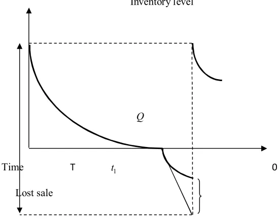
As depicted above, the inventory arrangement goes like this: Att0, opening replenishmentQunits are made, in whichSunits are delivered towards backorders, leaving a balance ofI_maxunits in the initial inventory. Fromt0tott₁time units, the inventory level depletes owing to both demand and deterioration. Att₁, the inventory level is zero. During the time (Tt₁)part of the shortage is backlogged and part of it is lost sales. Only the backlogging items are replaced by the after that replenishment.

Fig. 1. Inventory system of decaying item for declining market demand

The inventory function with respect to time can be determined by evaluating the differential equations

1

( )

( ) ( ) ( )

dI t

d t I t R t

dt    0 t t1

(1)

( )

dI t

DB t

dt   t1 t T

(2)

And with boundary conditions I(0)I_maxandI t( )₁ 0. The approximate solution of Eq. (1) by neglecting higher order term of



is









2 2

1 1

1

1 1

( )

2 2 1

t

t t

I t D t t   t t e 



  

   

 _   _  _  _



 

 

; 0 t t₁ ₍₃₎

Inventory level

Q

0 1

t

T

Time

(5)

Now, again taking the first two terms of the exponential series and neglecting the terms containing2

Eq. (4) becomes







 



2 2

1 1

1

1 1

( ) 1

2 2 1

t t

I t D t t   t t t

        _   _  _  _      

; 0 t t₁ ₍₄₎

So, the maximum inventory level for each cycle can be obtained as

2 1

1 1

max (0) ( ) 1

2 1

t t

I I I t D t









      _   _ 

  (5)

During the shortage interval



t T1,



, the demand at timetis partially backlogged at the fraction

( ) t

B t e Thus, the solution of differential Eq. (2) governing the amount of demand backlogged is as below

1

( )

( ) D T t T t

I t e  e 



 

 

  _  _ , t₁  t T ₍₆₎

with the boundary conditionI t( )₁ 0. LettTin Eq. (6), we obtain the maximum amount of demand backlogged per cycle as follows.

1

( )

( ) D 1 T t

S I T e 



 

 

   _  _.

(7)

Hence, the order quantity per cycle is given by

1

2 (1 )

( )

1 1

max 1 1

2 (1 )

T t

t t D

Q I S D t e

                _   _ _  _ 

  (8)

The order cost per cycle is

2

OCc . (9)

The deterioration cost per cycle is

1 1 1 0 ( ) t

DC c



t I t dt



_

( 1 ) ( 2 )

1 1

1

(1 ) ( 2 )

t t c D            _  _    

. ₍₁₀₎

The shortage cost per cycle is

1

3( ( )) T

t

SH

_

c I t dt





1 1 ( ) ( ) 3 1 1 ( ) T t T t e Dc

T t e

                    (11)

The opportunity cost per cycle is

1 ( ) 1 T T t t

OPC

_

_ e  _Ddt





1 ( ) 4 1 1 ( ) T t e c D T t

                (12)

4.1 Holding Cost

(6)

scenarios for discrete nature of variability of holding cost as retroactively variable holding cost and incrementally variable holding cost as:

Scenario 1: Retroactive holding cost; Scenario 2: Incremental holding cost;

4.1.1 Scenario 1: Retroactive Holding Cost

In this scenario, the unit holding cost per unit time is well thought-out as discrete in nature, and increases as the time in storage increases,h₁ h₂ h₃ ...h_n, for storage periods 1 through n, respectively. A retroactive holding cost implies that the holding cost of the last storage period is applied retroactively to all previous periods in the order cycle. That is, if the cycle length is



₁or less, the unit holding cost ish₁per time period; if the cycle length is between



₁  t



₂, all inventory (retroactively) is charged a holding cost ofh₂per unit per time period; etc. Since the same holding cost will be applied to all units in the cycle, we only need to determine the total inventory level for the entire order cycle:

1

0

( )

t

q

_

I t dt.

Therefore, holding cost is

1

0

( )

t

i

HCh I t dt

_

2 3 1 3

1 1 1 1

2 3 (1 )( 2) (1 )( 3)

i

t t t t

h D               _    _    

  (13)

whereh is the corresponding value ofhh_ifor



_i₁ t



_i. Thus, the average total costATC t1( )1 of

inventory cycle is

1( ) [1 1 ]

ATC t  OCHC DCSC OPC T

2 3 1 3

1 1 1 1 2

1( )1

2 3 (1 )( 2) (1 )( 3)

i

t t t t c T

D

ATC t h

T D  









      _ _    _       





1 1 ( ) ( 1 ) ( 2 )

( ) 3 1 1 1 1 1 ( )

(1 ) ( 2 )

T t

e c

t t

c T t e

                        _  _         _ _ (14)





1 ( ) 4 1 1 ( ) T t e

c D T t



                

In the first scenario, the objective is to determine the optimal values of shortage point t₁in order to minimize the average total cost ATC t₁( )₁ per unit time. The optimal solutionst₁*need to satisfy the following equation.

1 1

1 1 1

( )

( ) 0

dATC t D

f t

dt  T  ,

(15)

where

 



1



1 2

4 3

2 1 1 1

1( )1 1 1 1 1 1

(1 ) (1 )

T t

i

c c e

t t

f t h t t c t t

(7)

 





 1

1 3 4

1 3

( )

T t

T t c c e

T t c e

 



        .

Theorem 1 If 1T ,1



0 and 1then the solutions to Eq. (15) not only exists but also is unique (i.e., the optimal valuest is uniquely determined). ₁*

Proof: From (15), it is easily verified that, whenT 1and10 1

1 1 0

lim ( ) 0 t f t  and 1

1 1 lim ( ) 0. tT f t  Furthermore, taking first derivative off t₁( )₁ with respect tot₁(0, )T , we get df t₁( )₁ dt₁ 0.So,

1( )1

f t is a strictly increasing function oft₁(0, )T . It implies that the (15) is verified att₁ t₁*, with *

1

0t T, which is the unique root of f t₁( )₁ 0. This completes the proof.

Theorem 2 If 1T,10and



1 the average total cost per unit timeATC t₁( )₁ is convex and reaches its global minimum at point *

1

t .

Proof: From Eq. (15), if,1



T,1



0 we have

*

* ₁ ₁

1 1 2 1 1 1 1 2 1 ( )

( ) 0

t t t t

d ATC t D

f t

T

dt _ 

  

 

  . It implies,

* 1

t corresponds to the global minimum of convex

1( )1

ATC t . This completes the proof.

In this scenario, by usingt₁*, we can obtain the optimal maximum inventory level and the minimum average total cost per unit time from Eq. (5) and Eq. (14), respectively (we denote these values byI_max

andATC t₁( )₁* ). Furthermore, we can also obtain the optimal order quantity (we denote it byQ*) from Eq. (8).

4.1.2 Scenario 2: Incremental Holding Cost

In this scenario, the discrete incremental unit holding cost increases as the time in storage increases. In this situation, though, an incremental holding cost implies that the holding cost of each storage period is applied only to the units apprehended during that period. That is, if the positive inventory time length is



₁or less, the unit holding cost ish₁per time period; if the storage time-span is between



₁t₁ 



₂, the holding cost ofh₁is applied to the average inventory during the storage period from0to



₁andh₂is applied from



₁tot₁; etc. Thus, we require evaluating the average inventory level for each storage phase within the order cycle (note, for the last storage period,



_i is replaced witht₁):







 



1 2 2 1 1 1 1 1 1 1

( ) 2 2 1

i i i i i t D t

q D t t t t t dt

    













        _   _  _  _  



_ _ _  _ .

Therefore, holding cost per cycle is

2 1

1

( )

m

i i i i

i

HC h  _ q



_



1 1

2 1 2

1

1 1 1

1

( )

2 ( 1) ( 1) 2

m

i i

i i i

i

t t t

h D t t

                            _   _ _  _    _ _ _ _ 



(17)

















2 2 2 2 3 3 3 3

1 1 1 1

( 1)( 2) 2 6 2( 3)

i i i i i i i i

(8)

Thus, the average total costATC₂( )t₁ per unit time of inventory cycle is

2( )1 [ 2 ]

ATC t  OCHC DCSCOPC T

2 1

1 1

2 1 1 1

1

( ) ( )

2 ( 1)

m

i i i

i

t t

ACT t h t

T                  _   _    _ _ _ 











2 2 2 2

1 1 2

1 1

1

( )

( 1) 2 ( 1)( 2) 2

i i i i

i i t

t     _{ } _ _ _                     _  _   _ _   (18)









3 3 3 3 ₍₁ ₎ _{( 2} ₎

1 1 ₂ ₁ ₁

1

6 2( 3) (1 ) (2 )

i i i i c T t t

c D         _            _ _      _  _   __   __ 









1 1 1 ( ) ( ) ( ) 3

1 4 1

1 1

( ) ( )

T t T t

T t

e e

c

T t e c D T t

                                       .

In this scenario, the objective is to determine the optimal values of shortage point t1in order to

minimize the average total cost ATC₂( )t₁ per unit time. The optimal solutionst₁*need to satisfy the following equation.

2 1

2 1 1

( )

( ) 0

dATC t D

f t

dt  T  ,

(19)

where













1 1

2 1 1 1 1

1

(1 )

( ) 1

( 1)

e _i _i

i i i

i

t

f t h t t

                                



(20)  





 





  1 1 1 4 3

1 3 4

1 1 1 ( 1) 3

T t _{T t}

T t

c c e _c _c _e

c t t T t c e

 _            _ _         _  _   

Theorem 3 If _ _





_

_

1 1

1

1 4 3

1 1

1

( 1 )

e e _i _i _i

T T

i i i

i i

h

h c e c T e

             _ _          

  and10, then the

solutions to Eq. (19) not only exists but also is unique (i.e., the optimal values * 1

t is uniquely determined).

Proof: From Eq. (19), it is easily verified that, when _ _





_

_

1 1

1

1 4 3

1 1

1

( 1)

e e _i _i _i

T T

i i i

i i

h

h c e c Te

             _ _            

and10

1

2 1 0

lim ( ) 0

t f t  and1

2 1

lim ( ) 0.

tT f t  Furthermore, taking first derivative of f2( )t1 with respect tot₁( 0, )T , we get df₂( )t₁ dt₁0.So, f₂( )t₁ is a strictly increasing function oft₁( 0, )T . It implies that the (19) is verified att₁ t₁*, with0t₁*T, which is the unique root off₂( )t₁ 0. This completes the proof.

Theorem 4If _ _





_

_

1 1

1

1 4 3

1 1

1

( 1)

e e _i _i _i

T T

i i i

i i

h

h c e c Te

             _ _          

  and10, the average

total cost per unit timeATC2( )t1 is convex and reaches its global minimum at point

* 1

(9)

Proof:From Eq. (19), if













1 1

1

1 4 3

1 1

1

( 1)

e e _i _i _i

T T

i i i

i i

h

h c e c Te

 

 

  

 



 

 _ _



 



    





and10 we

have

*

* 1 1

1 1

2

2 1

2 1 2

1 ( )

( ) 0

t t t t

d ATC t D

f t T

dt _ 

  

 

  . It implies,

* 1

t corresponds to the global minimum of

convexATC2( )t1 . This completes the proof. In this scenario, by using * 1

t , we can obtain the optimal

maximum inventory level and the minimum average total cost per unit timeATC₂(t₁*) from (5) and (19), respectively. Furthermore, we can also obtain the optimal order quantity from (8).

5. Numerical Examples

As an illustration of both scenarios of developed model, a numerical example is presented for a single product. To perform the numerical analysis, data have been taken randomly from literatures in appropriate units.

Example 1: We consider an inventory system which verifies the described assumptions above. The input data of parameters are taken randomly as T 4,a0.4,b2,0.8,h₁0.4,h₂ 0.5,h₃ 0.6

0 1 2 3 1

2, 0, 1, 2, t

          d10,c₁ 3,c₂ 1,c₃3,R2,H0.4andc₄ 2.

By using MATHEMATICA 8.0, the global minimum Average Total Cost per unit timeATC t_i( )₁ ,

1, 2

i along with the optimal value of t1* is calculated for each the proposed i-th scenario. The Optimal Order Quantity(Q*) is also calculated in each scenario. The summary of crucial values for each scenario is given below.

Table 1

Summary of model's optimal values in i-th scenario No. of scenario *

1

t Q* ATC t_i(₁*)

1 1.543017 115.4670 344.737

2 1.584176 116.259 342.062

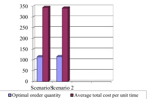
Observations: One can make following remarks.

i.The Optimal Average Total Cost per unit time is greater in the scenario 1. ii.The Optimal Order Quantity has maximum value in the scenario 2.

Fig. 2. Inventory model optimal values for each scenario

0 50 100 150 200 250 300 350

Scenario 1Scenario 2

(10)

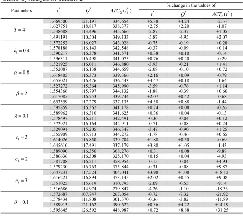
6. Sensitivity Analysis

In this section, the effects of studying the changes in the optimal value of Average Total Cost per unit time, the optimal shortage point and the optimal value of Order Quantity per cycle of each scenario with respect to changes in some model parameters are discussed. The sensitivity analysis in each scenario is performed by changing the value of each of the parameters by 5% and 10% , taking one parameter at a time and keeping the remaining parameters unchanged. Example 1 is used in each scenario.

6.1 Sensitivity Analysis for Scenario 1

To discuss the effect of changes of model parametersT h, ₁, , , ,   c c c₁, ₃, ₄and on the optimal value of the average total cost(ATC t₁(₁*)344.737) , the shortage time point(t₁* 1.543017)and the value of Order Quantity per cycle(Q* 115.4670) for scenario 1, the different values of these parameter according to5% and 10%change in each have taken and its effect onTAC t1( )1* ,

* 1

t andQ*are presented in the following Table 2.

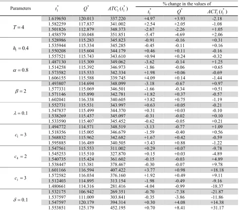
Table 2

Sensitivity Analysis for Scenario 1

Parameters t₁* Q* ATC t₁(₁*) * % change in the values of 1

t Q* ACT t1(1*)

4

T

1.619650 120.013 337.220 +4.97 +3.93 -2.18 1.582259 117.837 341.002 +2.54 +2.05 -1.08 1.501826 112.879 348.373 -2.67 -2.26 +1.05 1.458579 110.048 351.851 -5.47 -4.69 +2.06

1 0.4

h 

1.528986 115.283 345.823 -0.91 -0.16 +0.31 1.535944 115.334 345.285 -0.45 -0.11 +0.16 1.550208 115.604 344.179 +0.46 +0.11 -0.16 1.557521 115.743 343.610 +0.94 +0.24 -0.32

0.8



1.487130 115.309 349.062 -3.62 -0.14 +1.25 1.514258 115.392 346.973 -1.86 -0.06 +0.65 1.573582 115.533 342.334 +1.98 +0.06 -0.69 1.606155 115.588 339.745 +4.09 +0.14 -1.44

2



1.493807 114.694 348.099 -3.18 -0.67 +0.97 1.577331 115.069 346.501 -1.66 -0.34 +0.51 1.571146 115.890 342.781 +1.82 +0.37 -0.57 1.602041 116.338 340.605 +3.82 +0.75 -1.19

0.1



1.552731 115.531 343.997 +0.63 +0.05 -0.21 1.547837 115.499 344.370 +0.31 +0.03 -0.10 1.538269 115.437 345.097 -0.31 -0.02 +0.10 1.533590 115.407 345.452 -0.62 -0.05 +0.21

1 3

c 

1.494772 114.571 348.519 -3.13 -0.77 +1.09 1.518356 115.005 346.679 -1.59 -0.40 +0.56 1.568832 115.962 342.682 +1.67 +0.42 -0.59 1.595885 116.489 340.505 +3.43 +0.88 -1.22

4 2

c 

1.547561 115.553 311.002 +0.29 +0.07 -9.78 1.545253 115.510 327.870 +0.15 +0.03 -4.89 1.540735 115.424 361.602 -0.15 -0.03 +4.89 1.538447 115.381 378.467 -0.30 -0.07 +9.78

3 3

c 

1.601166 116.594 407.422 +3.77 +0.98 +18.18 1.572582 116.034 376.160 +1.92 +0.49 +9.11 1.512403 114.895 313.154 -1.98 -0.49 -9.16 1.480661 114.316 281.416 -4.04 -0.99 -18.37

0.1



(11)

Observations: From Table 2 the following observations can be made as:

1.ATC t₁(₁*) increases with increase in the values of model parametersh₁, , ,  c₁andc₃ whileATC t₁(₁*)

decreases with increase in the value ofT, ,



c₄and. ATC t₁(₁*)is highly sensitive to changes inT c c, ₃, ₄

and. It is less sensitive to changes in , andc₁; and very less sensitive to change inh₁and;

2. *

1(1)

ATC t decreases with decrease in the values of model parametersh₁, , ,  c₁andc₃ while * 1(1)

ATC t

increases with decrease in the value ofT, ,



c₄and. * 1(1)

ATC t is highly sensitive to changes inT c c, ₃, ₄

and. It is less sensitive to changes in , andc₁; and very less sensitive to change inh₁and;

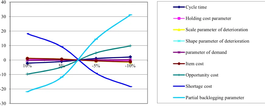
Fig. 3. Behavior of optimal average total cost per unit time in scenario 1

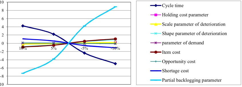
Fig. 4. Behavior of optimal ordering quantity in scenario 1

3.Q* increases with increase in the values of model parametersT, , c₃andc₄ whileQ*decreases with increase in the value ofh₁, , ,  c₁and. Q*is highly sensitive to changes inT and . It is less sensitive to changes inh₁, , c₁andc₃; and very less sensitive to change in , andc4;

-30 -20 -10 0 10 20 30 40

10% 5% -5% -10%

Cycle time

Holding cost parameter Scale parameter of deterioration Shape parameter of deterioration parameter of demand

Item cost Opportunity cost Shortage cost

Partial backlogging parameter

-10 -8 -6 -4 -2 0 2 4 6 8 10

10% 5% -5% -10%

Cycle time

Holding cost parameter

Scale parameter of deterioration

Shape parameter of deterioration

parameter of demand

Item cost

Opportunity cost

Shortage cost

(12)

4.Q* decreases with decrease in the values of model parametersT, , c₃andc₄ whileQ*increases with decrease in the value ofh₁, , ,  c₁and. Q*is highly sensitive to changes inT and. It is less sensitive to changes inh₁, , c₁andc₃; and very less sensitive to change in , andc4.

6.2 Sensitivity Analysis for Scenario 2

To discuss the effect of changes of model parametersT h, ₁, , , ,   c c c₁, ₃, ₄and on the optimal value of the average total cost(ATC₂(t₁*)342.062) , the shortage time point(t₁* 1.584176)and the value of Order Quantity per cycle(Q*116.259) for scenario 2, the different values of these parameter according to5% and 10%change in each have taken and its effect on *

2(1)

TAC t , * 1

t and *

Q are presented in the following Table 3.

Table 3

Sensitivity Analysis for Scenario 2

Parameters t₁* Q* ATC₂(t₁*)

% change in the values of

* 1

t Q* ACT t₂(₁*)

4

T

1.669500 121.191 334.654 +5.38 +4.24 -2.16 1.627751 118.817 338.377 +2.75 +2.20 -1.07 1.538688 113.496 345.666 -2.87 -2.37 +1.05 1.491191 110.504 349.133 -5.87 -4.95 +2.07

1 0.4 h 

1.572252 116.027 343.028 -0.75 -0.19 +0.28 1.578188 116.143 342.548 -0.37 -0.09 +0.14 1.590217 116.378 341.571 +0.38 +0.10 -0.14 1.596311 116.498 341.075 +0.76 +0.20 -0.29

0.8



1.521925 116.011 346.880 -3.93 -0.21 +1.41 1.552087 116.138 344.659 -2.08 -0.10 +0.72 1.618405 116.373 339.366 +2.16 +0.09 -0.79 1.655021 116.476 336.443 +4.47 +0.18 -1.64

2



1.527272 115.364 345.990 -3.59 -0.76 +1.14 1.554366 115.797 344.132 -1.88 -0.39 +0.60 1.617085 116.753 339.744 +2.07 +0.42 -0.68 1.653559 117.279 337.135 +4.38 +0.88 -1.44

0.1



1.595859 116.362 341.178 +0.74 +0.08 -0.26 1.589962 116.310 341.625 +0.36 +0.04 -0.13 1.578497 116.211 342.491 -0.36 -0.04 +0.12 1.572921 116.164 342.911 -0.71 -0.08 +0.24

1 3

c 

1.529091 115.205 346.347 -3.47 -0.90 +1.25 1.555909 115.713 344.272 -1.78 -0.46 +0.65 1.614026 116.850 339.704 +1.88 +0.50 -0.69 1.645610 117.491 337.179 +3.88 +1.05 -1.43

4 2

c 

1.589090 116.356 308.276 +0.31 +0.08 -9.88 1.586636 116.308 325.170 +0.15 +0.04 -4.93 1.581708 116.211 358.954 -0.15 -0.04 +4.93 1.579230 116.763 375.844 -0.31 -0.08 +9.87

3 3

c 

1.647231 117.524 404.041 +3.98 +1.08 +18.12 1.616221 116.894 373.145 +2.02 +0.55 +9.08 1.551025 115.619 310.795 -2.09 -0.55 -9.14 1.516686 114.974 279.847 -4.26 -1.10 -18.33

0.1



1.572687 107.747 267.054 -0.72 -7.32 -21.92 1.578434 111.808 301.370 -0.36 -3.82 -11.89 1.589913 121.162 390.622 +0.36 +4.22 +14.19 1.595645 126.592 448.987 +0.72 +8.88 +31.25

(13)

1.ATC₂(t₁*) increases with increase in the values of model parametersh₁, , ,  c₁andc₃ whileATC₂(t₁*)

decreases with increase in the value ofT, ,



c₄and. ATC₂(t₁*)is highly sensitive to changes inT c c, ₃, ₄

and. It is less sensitive to changes in , andc₁; and very less sensitive to change inh₁and.

2. *

2(1)

ATC t decreases with decrease in the values of model parametersh₁, , ,  c₁andc₃ while * 2(1)

ATC t

increases with decrease in the value ofT, ,



c₄and. * 2(1)

ATC t is highly sensitive to changes inT c c, ₃, ₄

and. It is less sensitive to changes in , andc₁; and very less sensitive to change inh₁and.

Fig. 5. Behavior of optimal average total cost per unit time in scenario 2

Fig. 6. Behavior of optimal ordering quantity in scenario 2

3.Q* increases with increase in the values of model parametersT, , c₃andc₄ whileQ*decreases with increase in the value ofh₁, , ,  c₁and. Q*is highly sensitive to changes inT and . It is less sensitive to changes inh₁, , c₁andc₃; and very less sensitive to change in , andc4.

4.Q* decreases with decrease in the values of model parametersT, , c₃andc₄ whileQ*increases with decrease in the value ofh₁, , ,  c₁and. *

Q is highly sensitive to changes inT and. It is less sensitive to changes inh₁, , c₁andc₃; and very less sensitive to change in , andc4.

-30 -20 -10 0 10 20 30 40

10% 5% -5% -10%

Cycle time

parameter of demand

Item cost

Opportunity cost

Shortage cost

Partial backlogging parameter

-10 -8 -6 -4 -2 0 2 4 6 8 10

10% 5% -5% -10%

Cycle time

parameter of demand

Item cost

Opportunity cost

Shortage cost

(14)

7. Conclusions

In this model, we have studied an inventory model in which the inventory is depleted not only by declining pattern of demand but also by Weibull distributed deterioration where holding cost per unit time is considered a discretely variable. Shortages are allowed and partially backlogged. Conditions for existence and uniqueness of the optimal solution have been provided. Therefore, the proposed model can be used widely in inventory-control of certain deteriorating items such as food items, electronic components, and fashionable commodities, and others. Moreover, the advantage of the proposed inventory model is illustrated with example. This study highlights that the optimal average total cost per unit time is high when holding cost per unit per unit time is considered as retroactively to all previous periods of storing and optimal value of ordered quantity is less. On the other hand, the optimal average total cost per unit time is less when holding cost per unit per unit time is considered as incremental to periods of storing and optimal value of ordered quantity is high. In future, this paper may be extended with stochastic demand and permissible delay of payment.

Acknowledgment

The author would like to sincerely thank the anonymous referees whose comments improved the earlier version of this paper.

References

Abad, P.L. (2000). Optimal lot size for a perishable good under conditions of finite production and partial backordering and lost sale. Computers & Industrial Engineering, 38, 457–465.

Aggarwal, S.P. (1978). A note on an order-level model for a system with constant rate of deterioration.

Opsearch, 15, 184-187.

Alfares, H.K. (2007). Inventory model with stock-level dependent demand rate and variable holding cost. International Journal of Production Economics, 108, 12, 259–265.

Bhunia, A. K. & Shaikh, A.A. (2011). A deterministic model for deteriorating items with displayed inventory level dependent demand rate incorporating marketing decisions with transportation cost.

International Journal of Industrial Engineering Computations, 2, 547–562.

Chang, H.J. & Dye, C.Y. (1999). An EOQ model for deteriorating items with time varying demand and partial backlogging. Journal of the Operational Research Society, 50, 1176–1182.

Dye, C.Y., Ouyang, L.Y., & Hsieh, T.P. (2007). Inventory and pricing strategies for deteriorating items with shortages: A discounted cash flow approach. Computers and industrial Engineering, 52, 29-40. Ferguson, M., Hayaraman, V. & Souza, G.C. (2007). Note: An application of the EOQ model with

nonlinear holding cost to inventory management of perishables. European Journal of Operational Research, 180, 1, 485–490.

Hollier, R.H. & Mak, K.L. (1983). Inventory replenishment policies for deteriorating items in a declining market. International Journal of Production Research, 21, 813–826.

Hou, K.L. (2006).An inventory model for deteriorating items with stock-dependent consumption rate and shortages under inflation and time discounting. European Journal of Operational Research, 168, 463- 474.

Hung, K.C. (2011).An inventory model with generalized type demand, deterioration and backorder rates. European Journal of Operational Research, 208, 239- 242.

Jaggi, C.K., Aggarwal, K.K., & Goel, S.K. (2006). Optimal order policy for deteriorating items With inflation induced demand. International Journal of Production Economics, 103, 707-714.

(15)

Khanra, S. Ghosh, S.K., & Chaudhuri, K.S. (2011). An EOQ model for a deteriorating item with time– dependent quadratic demand under permissible delay in payment. Applied Mathematics and Computation, 218, 1- 9.

Liao, J.J., & Huang, K.N. (2010).Deterministic inventory model for deteriorating items with trade credit financing and capacity constraints. Computers and Industrial Engineering, 59, 611-618. Lin, J. (2012). A demand independent inventory control. Yugoslav Journal of Operations Research, 22,

1-7.

Mishra, V.K. & Singh, L.S. (2011). Deteriorating inventory model for time dependent demand and holding cost with partial backlogging. International Journal of Management Science and Engineering Management, 6, 4, 267-271.

Park, K.S. (1982). Inventory models with partial backorders. International Journal of Systems Science, 13, 1313–1317.

Papachristos, S. & Skouri, K. (2000). An optimal replenishment policy for deteriorating items with time-varying demand and partial exponential type-backlogging. Operations Research Letters, 27, 175–184.

Papachristos, S. & Skouri, K. (2003). An inventory model with deteriorating items, quantity discount, pricing and time-dependent partial backlogging. International Journal of Production Economics, 83, 247–256.

Patra, S. K., Lenka, T. K., & Ratha, P.C. (2010).An order level EOQ model for deteriorating items in a single warehouse system with price dependent demand in non-linear form. International Journal of Computational and Applied Mathematics, 5(3), 277-288.

Sana, S.S. (2010). Optimal selling price and lot size with time varying deterioration and partial backlogging. Applied Mathematics and Computation, 217, 185- 194.

Skouri, K., Konstantaras, I., Papachristos, S., & Teng, J.T. (2011). Supply chain models for deteriorating products with ramp type demand rate under permissible delay in payments. Expert Systems with Applications, 38, 14861-14869.

Taleizadeh, A.A., Widyadana, G.A., Wee, H.M., & Biabani, J. (2011). Multi products single machine economic production quantity model with multiple batch size. International Journal of Industrial Engineering Computations, 2(2), 213-224.

Taleizadeh, A.A., Cárdenas-Barrón, L.E., Biabani, J., & Nikousokhan, R. (2012). Multi products single machine EPQ model with immediate rework process. International Journal of Industrial Engineering Computations, 3(2), 93-102.

Teng, J.T., Yang, H.L., & Ouyang, L.Y. (2003). On an EOQ model for deteriorating items with timevarying demand and partial backlogging. Journal of Operational Research Society, 54 (4), 432-436.

Teng, J.T., & Yang, H.L. (2004). Deterministic economic order quantity models with partial backlogging when demand and cost are fluctuating with time. Journal of the Operational Research Society, 55 (5), 495-503.

Teng, J.T., Oyang, L.Y., & Chen, L.H. (2007).A comparison between two pricing and lot-sizing models with partial backlogging and deteriorated items. International Journal of Production Economics, 105 (1), 190-203.

Tyagi, A.P., Pandey, R.K. & Singh, S.R. (2012). Optimization of inventory model for decaying item with variable holding cost and power demand. Proceedings of National Conference on Trends & Advances in Mechanical Engineering, ISBN: 978-93-5087-574-2, 774-781.

Tripathi, R.P. (2013). Inventory model with different demand rate and different holding cost.

International Journal of Industrial Engineering Computations, 4, 437–446.

Weiss, H.J. (1982). Economic order quantity models with nonlinear holding costs. European Journal of Operational Research, 9, 56–60.

Wee, H.M. (1995). A deterministic lot-size inventory model for deteriorating items with shortages and a declining market. Computers & Operations Research, 22, 345–356.

(16)

Yang, H.L. (2005).A comparison among various partial backlogging inventory lot-size models for deteriorating items on the basis of maximum profit. International Journal of Production Economics,

96 (1), 119-128.