Munich Personal RePEc Archive
Discrimination between deterministic
trend and stochastic trend processes
Caiado, Jorge and Crato, Nuno
2005
Online at
https://mpra.ub.uni-muenchen.de/2076/
and stochastic trend processes
Jorge Caiado1
and Nuno Crato2
1 Escola Superior de Ciˆencias Empresariais, Instituto Polit´ecnico de Set´ubal and CEMAPRE, Rua do Quelhas 6, 1200-781 Lisboa, Portugal, (e-mail: [email protected])
2 Instituto Superior de Economia e Gest˜ao, Universidade T´ecnica de Lisboa and CEMAPRE, Rua do Quelhas 6, 1200-781 Lisboa, Portugal, (e-mail: [email protected])
Abstract. Most of economic and financial time series have a nonstationary be-havior. There are different types of nonstationary processes, such as those with stochastic trend and those with deterministic trend. In practice, it can be quite difficult to distinguish between the two processes. In this paper, we compare ran-dom walk and determinist trend processes using sample autocorrelation, sample partial autocorrelation and periodogram based metrics.
Keywords: autocorrelation, classification, determinist trend, Kullback-Leibler, periodogram, stochastic trend, time series.
1
Introduction
There are different types of nonstationarity processes. One can consider a deterministic linear trend processyt=a+bt+εt(withεta white noise term),
that can be transformed into a stationary process by subtracting the trend
a+bt, and a stochastic linear trend process such as the so-called random walk model (1−B)yt=εtoryt=yt−1+εt. An interesting, but some times
difficult problem is to determine whether a linear process contains a trend, and whether a linear process exhibits a deterministic or a stochastic trend. In particular, it is useful to distinguish between a random walk plus drift
yt=µ+yt−1+εtand a deterministic trend in the formyt=a+µt+εt.
The problem of classifying and clustering time series has been studied by Piccolo (1990), Tong and Dabas (1990), Shaw and King (1992), Kakizawa, Shumway and Taniguchi (1998), Maharaj (2000, 2002), Caiado, Crato and
Pe˜na (2005), Xiong and Yeung (2004), among others. In this paper, we
2 Jorge Caiado and Nuno Crato
2
Classification Methods
A fundamental problem in clustering and classification analysis is the choice of a relevant metric. We know that the Euclidean distance is not a good metric for classifying time series since it is invariant to permutation of the coordinates and so it does not take into account the information about the autocorrelations.
LetX = (x1,t, . . . , xk,t)′ be a vector time series and ρbi = (bρi,1, . . . ,ρbi,m)
be a vector of the sample autocorrelations of the time seriesifor somemsuch thatρbk ∼= 0 fork > m. A distance between two time seriesxandycan be
de-fined byd(x, y) =p(ρbx−ρby)′Ω(ρbx−ρby), whereΩis some matrix of weights
(see Galeano and Pe˜na, 2000) . Caiado, Crato e Pe˜na (2004) proposed three possible ways of computing a distance by using the sample autocorrelation function (ACF). The first uses the Euclidean distance between the sample autocorrelations coefficient vectors with uniform weights (ACFU metric),
dACF U(x, y) =
v u u t L X j=1
(ρbj,x−ρbj,y)2, (1)
where L is the number of autocorrelations. The second uses the Euclidean
distance with geometric weights decaying with the lag (ACFG metric),
dACF G(x, y) =
v u u t L X j=1
fj(ρbj,x−ρbj,y)2, (2)
where fj =pqj for i= 1,2, ..., L, p= 1−q and 0< p <1. The third uses
the Mahalanobis distance between the autocorrelations (ACFM metric),
dACF M(x, y) =
q
(ρbx−ρby)′Ω−1(ρbx−ρby), (3)
where Ω is the sample covariance matrix of the autocorrelation coefficients given by Bartlett’s formula (see Brockwell and Davis, 1991, p. 221-222). A metric based on the sample partial autocorrelation function (PACF) is defined by
dP ACF(x, y) =
q
(φbx−φby)′Ω(φbx−φby), (4)
whereφbii are the sample partial autocorrelations andΩ is also some matrix
of weights.
A measure based on the Kullback-Leibler (KL) information for time series classification can be defined by
dKL(x, y) =tr(RxR−
1
y )−log |Rx|
where Rx and Ry are the sample autocorrelation matrices of time series x
andy. Since dKL(x, y)6=dKL(y, x), one can define a symmetric distance or
quase-distance (KLJ metric), known as theJ divergence, as,
dKLJ(x, y) =
1
2dKL(x, y) + 1
2dKL(y, x), (6)
which satisfies all the usual properties of a metric except the triangle inequal-ity.
Caiado, Crato and Pe˜na (2004) introduced also a periodogram-based
metric. Let x and y be observed time series with periodograms, Px(wj) =
n−1
|Pnt=1xte−itwj| 2
andPy(wj) =n−1|Pnt=1yte−itwj| 2
at frequencieswj=
2πj/n, j = 1, ..., m (with m = [(n−1)/2]) in the range 0 to π, and let
N P(wj) = P(wj)/bγ0 be the normalized periodogram (with bγ0 the sample
variance). Since the variance of periodogram ordinates is proportional to the spectrum value at the corresponding frequencies, Caiado, Crato and Pe˜na (2004) proposed a metric based on the logarithm of the normalized peri-odograms (LNPER metric),
dLN P ER(x, y) =
v u u t
m
X
j=1
[logN Px(wj)−logN Py(wj)]
2
. (7)
3
Monte Carlo Simulations
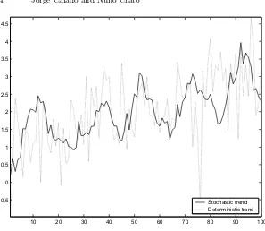
For the Monte Carlo simulations we chose the determinist trend and random walk plus drift models studied by Enders (1995, p. 252),
yt= 1 + 0.02t+εt
and
yt= 0.02 +yt−1+εt/3,
with εt a zero mean and unit variance white noise. These processes were
4 Jorge Caiado and Nuno Crato
10 20 30 40 50 60 70 80 90 100
-0.5 0 0.5 1 1.5 2 2.5 3 3.5 4 4.5
[image:5.595.136.433.97.355.2]Stochastic trend Deterministic trend
Fig. 1.Simulated stochastic trend and deterministic trend processes.
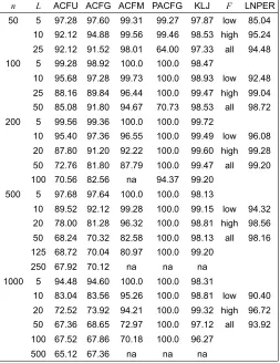
Table 1 presents the percentage of sucesses obtained in the comparison between the two processes, where n is the sample size, L is the autocorre-lation lenght, the sample autocorreautocorre-lation and sample partial autocorreautocorre-lation metrics (ACFG and PACFG metrics) uses a geometric decay of p= 0.05, in
the LNPER metricF for low frequencies corresponds to periodogram
ordi-nates from 1 to √n andF for high frequencies corresponds to periodogram ordinates from√n+ 1 ton/2.
n L ACFU ACFG ACFM PACFG KLJ F LNPER
50 5 97.28 97.60 99.31 99.27 97.87 low 85.04 10 92.12 94.88 99.56 99.46 98.53 high 95.24 25 92.12 91.52 98.01 64.00 97.33 all 94.48 100 5 99.28 98.92 100.0 100.0 98.47
10 95.68 97.28 99.73 100.0 98.93 low 92.48 25 88.16 89.84 96.44 100.0 99.47 high 99.04 50 85.08 91.80 94.67 70.73 98.53 all 98.72 200 5 99.56 99.36 100.0 100.0 99.72
10 95.40 97.36 96.55 100.0 99.49 low 96.08 20 87.80 91.20 92.22 100.0 99.60 high 99.28 50 72.76 81.80 87.79 100.0 99.47 all 99.20 100 70.56 82.56 na 94.37 99.20
500 5 97.68 97.64 100.0 100.0 98.13
10 89.52 92.12 99.28 100.0 99.15 low 94.32 20 78.00 81.28 96.32 100.0 98.81 high 98.56 50 68.24 70.32 82.58 100.0 98.13 all 98.16 125 68.72 70.04 80.97 100.0 99.20
250 67.92 70.12 na na na 1000 5 94.48 94.60 100.0 100.0 98.31
10 83.04 83.56 95.26 100.0 98.81 low 90.40 20 72.52 73.92 94.21 100.0 99.32 high 96.72 50 67.36 68.65 72.97 100.0 97.12 all 93.92 100 67.52 67.86 70.18 100.0 96.27
[image:6.595.169.422.138.466.2]500 65.12 67.36 na na na
Table 1. Percentage of sucess in the comparison between random walk plus drift and deterministic trend processes.
4
Discussion
6 Jorge Caiado and Nuno Crato
main differences arise for the first ACF and PACF values. Contrarily to what could be expected, the performance of ACF methods decreases with sample size. This does not happen with the PACF method. Kullback-Leibler method shows a remarkable good performance and stability across sample sizes and ACF orders considered. The periodogram-based metric compares well to Kullback-Leibler and is computationally simpler.
Acknowledgment: We thank Daniel Pe˜na of Universidad Carlos III
de Madrid for contributions in the development of the methods used in this paper. This research was supported by a grant from the Funda¸c˜ao para a Ciˆencia e Tecnologia (POCTI/FCT).
References
1.Brockwell, P. J. and Davis, R. A. (1991). Time Series: Theory and Methods, Springer, New York.
2.Caiado, J., Crato, N. and Pe˜na, D. (2005). ”A periodogram-based metric for time series classification”,Computational Statistics&Data Analysis(forthcoming). 3.Enders, W. (1995).Applied Econometric Time Series, Wiley, New York. 4.Galeano, P. and Pe˜na, D. (2000). ”Multivariate analysis in vector time series”,
Resenhas, 4, 383-404.
5.Kakizawa, Y., Shumway, R. H. and Taniguchi, M. (1998). ”Discrimination and clustering for multivariate time series”, Journal of the American Statistical Association, 93, 328-340.
6.Maharaj, E. A. (2000). ”Clusters of time series”, Journal of Classification, 17, 297-314.
7.Maharaj, E. A. (2002). ”Comparison of non-stationary time series in the frequency domain”,Computational Statistics &Data Analysis, 40, 131-141.
8.Piccolo, D. (1990). ”A distance measure for classifying ARIMA models”,Journal of Time Series Analysis, 11, 152-164.
9.Shaw, C. T. e King, G. P. (1992). ”Using cluster analysis to classify time series”,
Physica D, 58, 288-298.
10.Tong, H e Dabas, P. (1990). ”Cluster of time series models: an example”,Journal of Applied Statistics, 17, 187-198.
11.Xiong, Y. e Yeung, D. (2004). ”Time series clustering with ARMA mixtures”,