The Effects of Interim Performance Evaluations under Risk Aversion

Munich Personal RePEc Archive

The Effects of Interim Performance

Evaluations under Risk Aversion

Yurday, Zeynep

University of Rochester

September 2003

Online at

https://mpra.ub.uni-muenchen.de/1611/

The E

ff

ects of Interim Performance Evaluations

under Risk Aversion

by Zeynep Yurday

September 2003

Abstract

This paper reconsiders the applicability of a recently posed theoreti-cal result concerning the optimality of not providing interim performance evaluations to the agent when implementing a given amount of total effort. The model used by Lizzeri, Meyers and Persico (2002) under the assump-tion of a risk neutral agent restricted by limited liability is analyzed when the agent is risk averse to show that interim performance evaluations do matter in reducing contract costs. In particular, they enable the princi-pal to transfer the burden of insuring the agent against risk to the agent herself. Hence, the same incentives can be provided without as much consumption smoothing once performance information is revealed. On the other hand, when the incentive scheme isfixed, the risk averse agent mayfind it optimal to exert a greater amount of effort when performance evaluations are not revealed so as to insure herself against the possible losses that come with unexpected bad outcomes.

1

Introduction

In a dynamic principal-agent relationship where the principal is more informed compared to the agent about her performance, it is a natural question to ask, what the effect of disclosing such information to the agent is. In particular, how does revelation of such information affect the effort level chosen by the agent and how does it affect the contract cost the principal must incur in order to implement a given level of effort?

Real life examples necessitating such a question to be theoretically resolved abound. Consider, the relationship between a teacher and a student in the classroom: a teacher who is experienced in assessing the performance of a child based on her in-class participation, test scores and interaction with other

∗_{Department of Economics, University of Rochester, Rochester, NY 14627, USA. E-mail:}

students is in a better position to objectively evaluate how well a student is doing in the class; whereas a student who has just been introduced to the process of grappling with foreign concepts may not be aware of how well she is at learning them. Hence, the disparity in the position of the teacher and his student places the teacher at an informational advantage regarding the performance of the student. Given this informational asymmetry, how would the student react over time to learning about the assessment of her teacher? Will she start working more or less depending on whether she did well last week? And will she need to be given more points to study just as hard had she not known what her performance level was?

Perhaps the cost of rewarding the student for the amount of work she puts in is not so important for the teacher when the rewards are defined as course grades. However, once we consider the same informational asymmetry applied to the relationship between an employer and an employee in an organization, we realize that the principal’s valuation is not just based on getting the maximum amount of effort possible from the agent, but also on how costly it will be for him to have the agent exert that effort. That is, an employer’s concerns regarding the wages he has to pay his employee in order to make him work just as hard might prevent him from revealing performance information to his employee.

Lizzeri, Meyer, and Persico, (2002, henceforth LMP) analyze this question closely in a two-period, two-output, principal-agent model where both the prin-cipal and the agent are risk-neutral, and inefficiencies in effort provision exist due to limited liability on the part of the agent. Together with these assump-tions, they are able to show that even though the agent is willing to exert more effort under revelation of performance information, it is costlier to have her exert the same level of effort. In fact, for any amount of aggregate effort the principal wishes to implement, the contract cost under information revelation will always exceed that under no revelation.

Risk neutrality together with limited liability is key to establishing their conclusions. It is well known in the contract theory literature that with these assumptions, the optimal output-contingent wage contract will only award the most successful outcome while punishing—to the extent permitted by the degree of limited liability—the rest of the possible outcomes. When no performance information is revealed across time, the dynamic relationship between the prin-cipal and the agent is equivalent to that of a static one, where the agent commits to a sequence of efforts from the beginning and is compensated for the outcome to each at the end. The principal can therefore implement a given sequence of efforts at the least cost by simply rewarding the outcome that is most informa-tive about this sequence of efforts (usually the highest outcome if the maximum likelihood ratio property holds).

paying the agent positive wages for two sequential successes while paying her zero wages otherwise. By so doing, the principal is actually maximizing the incentive provision effect at the minimal cost possible. If information is revealed to the agent however, such a strong incentive provision mechanism may no longer implement the same effort level. Once a failure is revealed after thefirst period, if zero wages are awarded to the agent for any combination of outcomes involving a failure, then the agent will exert zero effort in the second period knowing that he will receive nothing. Hence, information revelation makes incentive provision more costly, by necessitating an increase in wages in order to provide the same aggregate effort level.

This paper shows that introducing another form of inefficiency which is due to risk aversion rather than limited liability has potential to alter the above conclusions completely. Namely, if the agent is risk averse, the optimal contract will involve a trade-offbetween incentive provision and insurance provision, and so even when no performance information is revealed, it will no longer be optimal to provide such strong incentives since it increases the amount of risk the agent will have to bear. In fact, the agent’s risk aversion will force the principal to insure the agent against risk by smoothing her consumption across different states. This insurance effect will have a stronger impact on the optimal contract under no revelation compared to revelation, since the agent is able to insure herself against risk by adjusting her second period effort level once performance information is revealed.

Such an outcome is intuitive when we think of the teacher-student relation-ship discussed above. The LMP (2002) result suggests that the teacher may implement the same amount of effort with lower grades by only offering afinal exam for the course. However, it is a well known fact that midterm exams which reveal the students’ performance are frequently used. A midterm exam may help adjust a student’s effort upon observing her intermediate performance level. Considering the student is risk averse, such an adjustment will remove the responsibility offthe teacher of actually insuring the student against a failure on thefinal exam. Such an insurance would be provided through a reduction in the dispersion of final grades across different performance levels. Had the student some idea regarding how well she was doing in the course prior to re-ceiving herfinal grade, she would have been able to insure herself by working harder and be better prepared to face the possibility of a low grade.

In what follows, we will recount the LMP (2002) model and show explicitly how the results will change once the agent is risk averse. Section 2 provides an outline of the model used; section 3 illustrates the effect interim performance evaluations have on the agent’s effort level for afixed incentive scheme; section 4 gives the necessary and sufficient conditions for the optimal incentive mechanism the principal wishes to offer, and presents comparative statics results comparing the optimal scheme when information is revealed and not revealed to the agent; section 5 gives computational results illustrating the theoretical results obtained;

2

The Model

The model is as presented in LMP (2002) with the exception of assuming a risk averse agent. Namely, there are two periods, with two possible outcomes each period given byxt∈{f, s}, wheref denotes failure andsdenotes success each

period. The agent exerts a one-dimensional effortet∈[0,1]each period. The

probability of a success in each periodtis equal to the level of effortet. Hence,

Pr(xt=s) =etand Pr(xt=f) = (1−et), where probabilities are independent

across periods. In each period, the cost of effort is denoted byc(et), wherec(.)

isC3_{, c}0_{(.)>0,and c}00_{(.)>0. To ensure an interior solutionc(0) =c}0_{(0) = 0}

andc0_{(1) =∞.}

Finally, the principal is assumed risk neutral, while the agent is risk averse with his utility function over wagesu(w(x1, x2)) being C3 such thatu0(.)>0

andu00_{(.)<0. The inverse utility function corresponding tou(.)will then be}

w(x1, x2) =h(u(x1, x2)) with h0(.)>0 and h00(.)> 0. The concavity of the

principal’s problem against a convex constraint set will be guaranteed once we convert the problem to one of solving for the optimal incentive scheme in terms of utilities ala Grossman and Hart (1983). Therefore, we define the optimal contract by a set of utility rewards conditional on all possible combinations of outcomes, namelyu= (u(s, s), u(s, f), u(f, s), u(f, f))∈R4_.

3

E

ff

ect of IPEs for a Fixed Incentive Scheme

3.1

Agent’s Problem

Assume for the remainder of this section that the principal has already decided on an incentive scheme u _∈ R4 _{to offer the agent. We will now define the}

agent’s problem of choosing an optimal effort sequence and compare the different effects a given incentive mechanism can have depending on the informational environment involved.

As in LMP (2002), we will compare two situations that may arise when the principal is more informed regarding the agent’s performance after thefirst period. In thefirst case called “No Revelation” denoted by the superscriptN, the agent chooses his second period efforteN

2 without observing herfirst period

outcome, and so is solving for the optimal {eN

1, eN2 }given the reward scheme

of the principal at the beginning of time. The agent’s payofffor an arbitrary level of effort can be written as follows:

UN_(e

1, e2)

−c(e2)]−c(e1)

Choosing the optimal effort pair {eN

1, eN2 }that maximizes the No Revelation

payoffimplies solving the following first order conditions for UN _{with respect}

toe1, e2:

∂UN

∂e1 : [e

N

2u(s, s) + (1−eN2)u(s, f)]−[eN2 u(f, s) + (1−eN2)u(f, f)] =c0(eN1)

∂UN

∂e2 : [e

N

1u(s, s) + (1−eN1)u(f, s)]−[eN1u(s, f) + (1−eN1)u(f, f)] =c0(eN2)

In the second case called “Revelation” denoted by the superscript R, the principal provides information to the agent regarding her performance after the

first period. Hence, the agent chooses her second period effort conditional on herfirst period outcome, namely the set©eR

2(f), eR2(s)

ª

. Once she solves for her second period effort, working backwards she chooses herfirst period efforteR

1.

Given the reward scheme of the principal, the agent’s payoffunder Revelation for an arbitrary effort level can be written as follows:

UR_(e

1, e2(s), e2(f))

=e1[e2(s)u(s, s) + (1−e2(s))u(s, f)−c(e2(s))] + (1−e1)[e2(f)u(f, s)

+(1₋e2(f))u(f, f)−c(e2(f))]−c(e1)

Once again the agent solves for the optimal effort level that maximizes her Revelation payoff using the first order conditions for UR _{with respect to}

e1, e2(s),ande2(f):

∂UR

∂e1 : [e

R

2(s)u(s, s) + (1−eR2(s))u(s, f)−c(eR2(s))]

−[eR

2(f)u(f, s) + (1−eR2(f))u(f, f)−c(eR2(f))] =c0(eR1)

∂UR

∂e2(s): [u(s, s)−u(s, f)] =c

0_(eR

2(s))

∂UR

∂e2(f) : [u(f, s)−u(f, f)] =c

0_(eR

2(f))

3.2

Characterizing Optimal E

ff

ort Levels

Assume as in LMP (2002) that thefixed incentive schemeu_∈R4_{is chosen such}

that u(s, f) =u(f, s) = u(s). Such a scheme will actually be optimal for the principal under No Revelation given that the agent’s effort choice is symmetric across the two periods. Likewise, provided that the principal chooses to provide linear incentives as defined, the agent’s problem under No Revelation will also be symmetric ine1 and e2 as can be observed from the first order conditions

(∂U_∂eN₁ ,∂U_∂eN₂ ) above. The agent’s optimal choice ofeN

1 andeN2 will therefore be

As in LMP (2002) wefirst characterize what happens to second period effort for a given first period probability of success. Note that the assumptions on

c0_{(.)are key in determining the results.}

Proposition 1 Given a fixed incentive scheme u = {u(s, s), u(s), u(f, f)} if thefirst period probability of success isfixed atpunder both Revelation and No Revelation, then if c0_{(.) is convex e}N

2 ≥ E(eR2) holds; and if c0(.) is concave

eN

2 ≤E(eR2)holds, with strict equality occuring if c0(.)is linear.

Proof. The agent’sfirst order condition with respect toe2 under No

Reve-lation suggests that when thefirst period probability of success isfixed:

p(u(s, s)₋u(s)) + (1₋p)(u(s)₋u(f, f)) =c0(eN₂ )

while her first order conditions with respect toe2(s)ande2(f)under

reve-lation suggests that:

u(s, s)−u(s) = c0(eR₂(s))

u(s)₋u(f, f) = c0(eR₂(f))

Provided eR

1 = p,we can combine the above as follows using Jensen’s

in-equality:

c0(eN₂ ) = p(u(s, s)₋u(s)) + (1₋p)(u(s)₋u(f, f)) = pc0_(eR

2(s)) + (1−p)c0(eR2(f))

= E(c0(eR₂)|p)

≥ c0(E(eR₂|p))ifc0(.)is convex_⇒eN_{2 ≥}E(eR₂|p)

≤ c0(E(eR₂|p))ifc0(.)is concave⇒eN₂ ≤E(eR₂|p) = c0(E(eR₂|p))ifc0(.)is linear_⇒eN₂ =E(eR₂|p)

To avoid the possible effects that convexity assumptions on c0_{(.) can have}

on second period effort, we now assume linear marginal costs of effort. For simplicity let c(e) = k₂e2 _{with c}0_{(e) = ke. The optimal second period effort}

under Revelation based on the solution to the system of first order conditions forUR _is:

eR₂(s) = u(s, s)−u(s)

k (1)

eR₂(f) = u(s)−u(f, f)

k (2)

Plugging these into thefirst order condition fore1 we can obtain,

eR₁ = 1

2k2([u(s, s)−u(s)]

2_{−[u(s)−u(f, f)]}2_{) +}u(s)−u(f, f)

On the other hand, the optimal first and second period effort under No Revelation is the solution to the symmetric system offirst order conditions for

UN _{obtained as follows:}

eN₂ = e

N

1(u(s, s)−u(s)) + (1−eN1)(u(s)−u(f, f))

k (4)

eN₁ = e

N

2(u(s, s)−u(s)) + (1−eN2)(u(s)−u(f, f))

k (5)

eN₁ = eN₂ = u(s)−u(f, f)

k₋[(u(s, s)₋u(s))₋(u(s)₋u(f, f))] (6)

Lemma 1 Given quadratic costs of effort c(e) = k₂e2_{, and a fixed}

incen-tive scheme defined by u = {u(s, s), u(s), u(f, f)}, if the agent chooses effort optimally in thefirst and second period, then

(i) an interior solution of effort under Revelation and No Revelation is guar-anteed if k > u(s, s)₋u(s)and k > u(s)₋u(f, f)

(ii) eN

1 =eN2 <(>)12 iff [u(s, s)−u(s)] + [u(s)−u(f, f)]<(>)k

Proof. Definex=u(s, s)₋u(s)andy=u(s)₋u(f, f)

Part (i): obvious foreR

2(s), eN2 (f)by (1) and (2), and foreN1 =eN2 which is

a convex combination ofxandy as defined by (4) and (5). ThateR

1 <1is less

straightforward.

(a) Ifx > y,then sincey < kandx < k

(x+y)(x−y) < 2k(x−y)<2k(k−y)

⇒ x2₋y2<2k2₋2ky

⇒ 0<x

2_−y2

2k2 +

y k <1

⇒ 0< eR₁ <1

(b) Ifx < y, then sincey < kandx < k

(x+y)(y₋x) < 2k(y₋x)<2ky

⇒ 0< x2−y2+ 2ky

⇒ 0<x

2_−y2

2k2 +

y k <

y k <1

⇒ 0< eR

1 <1

The last line follows from the solution toeR

1 given by (3).

Part (ii):

if eN = y

k₋[x₋y] <(>) 1 2

⇔ 2y <(>)k₋[x₋y]

⇔ y <(>)k₋x

Note that in order to obtain an interior solution for the optimal first and second period effort levels when the cost of effort is quadratic, the only re-quirement is that k > u(s, s)₋u(s) and k > u(s)₋u(f, f). LMP (2002) makes an implicit inference that k > u(s, s)₋u(s) implies k > [u(s, s)₋

u(s)]+ [u(s)₋u(f, f)]simply because the optimal No Revelation contract under risk neutrality with limited liability only rewards the most successful outcome, thereby makingu(s) =u(f, f) = 0. However, once this assumption is removed

k >[u(s, s)₋u(s)]+[u(s)₋u(f, f)]is not guaranteed. As a result, risk aversion makes it possible for the agent to exertfirst and second period effort eN > 1₂,

whenk <[u(s, s)₋u(s)]+[u(s)₋u(f, f)],while under risk neutrality the optimal No Revelation effort was such thateN< 12 always held.

In particular, Lemma 1 illustrates that eN > 1₂ is likely to be observed,

when the principal finds it optimal to equate the expected returns following a success and a failure, or in other words smoothes consumption across the different possible states. As we shall see in the section to follow this occurs when the agent becomes increasingly risk averse. Hence, in order to be able to implement a high amount of effort, exceeding 1

2 in each period, the agent must

be substantially risk averse relative to her cost of effort parameter such that the principal compensates the agent highly following both an initial success and an initial failure.

We now compare thefirst period effort levels under Revelation and No Reve-lation. Define the second period continuation payoffs conditional onfirst period output byvN(f), vN(s)andvR(f), vR(s)for the No Revelation and Revelation cases respectively. Thefirst order conditions for the agent’s problem under No Revelation and Revelation suggest that:

vN_(s)−vN_{(f) = c}0_(eN

1 ) (7)

vR(s)₋vR(f) = c0(eR₁) (8) where the LHS of each equation denotes the marginal benefit of exerting an additional increment of first period effort. LMP (2002) compare e1 under

the two scenarios by comparing the marginal benefits of each given a fixed probability of successpin thefirst period. The following Lemma replicates the argument for the risk averse agent.

Lemma 2 (LMP, 2002) For a fixed probability of success p in the first period and a quadratic cost of effort function, given that the agent chooses his effort optimally in the second period, vN_(s)−vN_{(f) ≤ (≥) v}R_(s)−vR_{(f) iff}

p_≤(_≥)1

2. Equality will hold only if u(s, s)−u(s) =u(s)−u(f, f)or p= 12

Proof. Define x = u(s, s)₋u(s) and y = u(s)₋u(f, f) and insert the optimal second period efforts under Revelation, eR

(2) respectively intovR_(s)−vR_{(f)to get:}

vR(s)−vR(f) = 1 2k(x

2_−y2_{) +y (9)}

and the optimal second period effort under No Revelation,eN

2 given by (6)

but for afixedfirst period probability of successpintovN_(s)−vN_{(f) :}

vN(s)₋vN(f) =

µ

px+ (1₋p)y k

¶

(x₋y) +y (10)

Subtracting (10) from (9) yields:

1

k

µ

1 2−p

¶

(x−y)2=k(eR₁ −eN₁) (11)

which implies that if

p_≤(_≥)1 2⇒e

N

1 ≤(≥)eR1

where equality holds when eitherp= 1

2 orx=y

Using the Lemmas above, we have the following proposition comparingfirst and second period efforts under Revelation and No Revelation.

Proposition 2 Suppose the agent is given a fixed incentive scheme, and a quadratic effort cost given by:

u={u(s, s), u(s), u(f, f)}withx=u(s, s)−u(s) andy=u(s)−u(f, f)

c(e) = k₂e2_{,where k > x, k > yso as to ensure interior solutions for effort}

Then,

(i) if x > yandk < x+y, theneN

1 > eR1 >12. Also,e2N> E(eR2|eR1)

(ii) ifx > y andk > x+y, theneN

1 < eR1 < 12. Also, e2N < E(eR2|eR1)

(iii) if x < y and k < x+y, then either eN

1 > eR1 > 12 or eN1 > 12 > eR1.

Also,eN

2 < E(eR2|eR1)

(iv) if x < y and k > x+y, then either eN

1 < eR1 < 12 or eN1 < 12 < eR1.

Also,eN

2 > E(eR2|eR1)

Proof. From (3), we already know that, for quadratic effort costsfirst period effort can be written as follows:

eR

1 =

1

2k2(x−y)(x+y) +

y k

While by (1), (2) and (4), the second period efforts are:

eN₂ = e

N

1 x+ (1−eN1)y

k

E(eR₂|eR₁) = e

R

1x+ (1−eR1)y

Part (i): ifx > yand k < x+y,then

eR₁ > 1

2k(x−y) + y k =

x+y

2k >

1 2

Combining Lemma 1 and 2, we know thatk < x+y ⇒eN

1 >12 ⇒eN1 > eR1.

Hence, eN₁ > eR₁ > 1₂. By the definition of eN₂ and E(eR₂|eR₁), x > y and

eN

1 > eR1 ⇒eN2 > E(eR2|eR1)

Part (ii): ifx > y andk > x+y,then

eR₁ < 1

2k(x−y) + y k =

x+y

2k <

1 2

Once again by Lemma 1 and 2,k > x+y _⇒ eN

1 < 12 ⇒eN1 < eR1. Hence,

eN

1 < eR1 <12. Also,x > yandeN1 < eR1 ⇒eN2 < E(eR2|eR1)

Part (iii): ifx < y andk < x+y,then

eR₁ < 1

2k(x−y) + y k =

x+y

2k >

1 2

Therefore, while k < x+y ⇒ eN

1 > 12 ⇒ eN1 > eR1 is known, either eN1 >

eR

1 >12 oreN1 > 12 > eR1 can hold. Also,x < yandeN1 > eR1 ⇒eN2 < E(eR2|eR1)

Part (iv): ifx < yandk > x+y,then

eR₁ > 1

2k(x−y) + y k =

x+y

2k <

1 2

Hence, whilek > x+y_⇒eN

1 < 12 ⇒eN1 < e1R is known, eithereN1 < eR1 <12

oreN

1 < 12 < eR1 can hold. Also, x < yandeN1 < e1R⇒eN2 > E(eR2|eR1)

The above analysis shows that counter to the results obtained by LMP (2002), when the agent is risk averse, it is possible for her to optimally ex-ert a high amount of effort under no information revelation exceeding 1₂. When this is true, the agent in fact exerts a higher amount offirst period effort under No Revelation compared to Revelation, while she also exerts a higher amount of second period effort providedu(s, s)−u(s)> u(s)−u(f, f)as the definitions of

eR

2(.)andeN2 reveal. This implies that when thefixed incentive scheme awards

a higher reward after a success compared to a failure, total effort under Reve-lation will be higher if total effort under No Revelation is less than 1, while the total effort under Revelation will be lower if total effort under No Revelation is greater than 1.

However, if the optimal contract has u(s)₋u(f, f) > u(s, s)₋u(s) then

eN

1 < eR1 ⇒eN2 > E(eR2|eR1) instead since the second period incentive to exert

u(s, s)₋u(s)> u(s)₋u(f, f). Since there is no trade-offbetween insuring the agent and providing her with incentives, it becomes optimal for him to spread incentives by increasing the expected rewards following a success. As we shall see in the next section, this doesn’t necessarily apply when the agent is risk averse. The necessity to insure the agent against risk may have the principal reward her more for a second period success following afirst period failure.

Having characterized the optimal effort provision for afixed incentive scheme under different circumstances, we now look at the optimal contract choice of the principal to determine when it is optimal to reward the agent more following a success or a failure. We will show in particular that the answer depends on the convexity assumptions used for the derivative of the inverse utility function,

h0_{(.). Finally, we will also show that the LMP (2002) result can be reversed,}

and that the optimal contract implementing afixed amount of total effort under Revelation can be less costly for the principal compared to the optimal contract under No Revelation.

4

Solving for the Optimal Incentive Scheme

4.1

Principal’s Problem

The principal’s problem can be written to maximize the difference in expected output and wage cost subject to the agent’s incentive compatibility and par-ticipation constraints, which guarantee that the agent does not deviate from the effort level chosen by the principal, and that she also finds it optimal to participate.

Thefirst order conditions of the agent’s problem as provided in the previous section are both necessary and sufficient to guarantee incentive compatibility with respect to the effort level chosen by the principal1_{. The participation}

constraint is satisfied as long as the chosen contract gives the agent a payoff

greater than or equal to herfixed outside option given byU .¯

We can combine these constraints together with the principal’s objective function to obtain a Lagrangian function under the No Revelation and Revela-tion scenarios as follows:

1_{The “first-order approach” is valid as long as the agent’s problem is globally concave} in effort. For a two-period principal-agent model with binary output levels, this condition is satified whenc000_{(.)>0for all effort levels, which is assumed for the remainder of the analysis.}

4.1.1 No Revelation Problem

£N _{= max}

{u(.),e1,e2}

⎧ ⎨ ⎩

[e1+e2]

−e1[e2h(u(s, s)) + (1−e2)h(u(s, f))]

−(1₋e1)[e2h(u(f, s)) + (1−e2)h(u(f, f))]

⎫ ⎬ ⎭

+µ₁n∂UN

∂e1

o

+µ₂n∂UN

∂e2

o

+λN{e1[e2u(s, s) + (1−e2)u(s, f)]

+(1₋e1)[e2u(f, s) + (1−e2)u(f, f)]−c(e1)−c(e2)−U¯}

where µ₁ and µ₂ denote the multipliers for the agent’s incentive compati-bility constraints in the first and second period respectively, and λN denotes the multiplier for the agent’s participation constraint. Maximizing £N _with

respect tou(.)for a given effort levele= (e1, e2)and simplifying to eliminateµ1

andµ₂, we obtain the following conditions which uniquely solve for the optimal contractuN_{(.)and multiplierλ}N _{under No Revelation:}

(i)e1[e2h0(uN(s, s)) + (1−e2)h0(uN(s, f))

+(1₋e1){e2h0(uN(f, s)) + (1−e2)h0(uN(f, f))] =λN

(ii)h0_(uN_{(s, s))−h}0_(uN_{(s, f)) =h}0_(uN_{(f, s))−h}0_(uN_{(f, f))}

(iii)e2[uN(s, s)−uN(f, s)] + (1−e2)[uN(s, f)−uN(f, f)] =c0(e1)

(iv)e1[uN(s, s)−uN(s, f)] + (1−e1)[uN(f, s)−uN(f, f)] =c0(e2)

(v)e1[e2uN(s, s) + (1−e2)uN(s, f)]

+(1₋e1)[e2uN(f, s) + (1−e2)uN(f, f)]−c(e1)−c(e2) = ¯U

We now present some preliminary implications that can be drawn from the

first order conditions above and the properties ofh(.)andh0_{(.). These results}

will be used in comparing the optimal contract cost under Revelation vs. No Revelation in the Proposition to follow.

Lemma 3If the principalfinds it optimal to implement eN

1 =eN2,then the

optimal contract will have uN_{(s, f) =u}N_{(f, s)under No Revelation.}

Lemma 4 Given that inverse utility function h(.) is three times diff eren-tiable, and u(s, f) =u(f, s)then

h0(u(s, s))−h0(u(s, f)) =h0(u(f, s))−h0(u(f, f))

implies

(ii) u(s, s)₋u(s, f)_≥u(f, s)₋u(f, f)if h0_{(.)is concave}

(iii) u(s, s)−u(s, f) =u(f, s)−u(f, f)if h0_{(.)is linear}2

(iv) under No Revelation the optimal effort choice will be such that eN

1 =eN2

Proof. Part (i): The convexity ofh0_{(.)implies that}

h0_{(u(s, s))−h}0_{(u(s, f)) ≥ h}00_{(u(s, f))[u(s, s)−u(s, f)]}

h0(u(f, s))−h0(u(f, f)) ≤ h00(u(f, s))[u(f, s)−u(f, f)]

sinceh00_{(u(s, f)) =h}00_{(u(f, s))>0, we have:}

u(f, s)₋u(f, f) _≥ h

0_{(u(f, s))−h}0_{(u(f, f))}

h00_{(u(f, s))} =

h0_{(u(s, s))−h}0_{(u(s, f))}

h00_{(u(s, f))} ≥u(s, s)−u(s, f)

⇒ u(s)₋u(f, f)_≥u(s, s)₋u(s)

Part (ii): the inequalities can be reversed when h0_{(.)is concave. Hence, it}

can be shown thatu(s, s)₋u(s)_≥u(s)₋u(f, f)

Part (iii): the linearity ofh0_{(.)would make the inequalities hold as equalities.}

Part (iv): conditions (iii) and (iv) under the No Revelation scenario can be rewritten as:

e2∆u(s) + (1−e2)∆u(f) = c0(e1)⇒eN1(e2)

e1∆u(s) + (1−e1)∆u(f) = c0(e2)⇒eN2(e1)

Since the two incentive compatibility conditions fore1ande2are symmetric,

we have:

eN₁(e2) =eN2(e1)⇒eN1 =eN2

4.1.2 Revelation Problem

£R_{= max}

{u(.),e1,e2(s),e2(f)}

⎧ ⎨ ⎩

[e1+e1e2(s) + (1−e1)e2(f)]

−e1[e2(s)h(u(s, s)) + (1−e2(s))h(u(s, f))]

−(1₋e1)[e2(f)h(u(f, s)) + (1−e2(f))h(u(f, f))]

⎫ ⎬ ⎭

+µ₁n∂UR

∂e1

o

+µ₂(s)n ∂UR

∂e2(s)

o

+µ₂(f)n ∂UR

∂e2(f)

o

+λR{e1[e2(s)u(s, s) + (1−e2(s))u(s, f)−c(e2(s))]

+(1₋e1)[e2(f)u(f, s) + (1−e2(f))u(f, f)−c(e2(f))]−c(e1)−U¯}

where µ₁, µ₂(s), µ₂(f) denote the multipliers for the agent’s incentive com-patibility constraints with respect tofirst and second period efforts respectively, andλRdenotes the multiplier for the agent’s participation constraint. Similarly, maximizing£R_{with respect tou(.)for a given e}ff_{ort levele= (e1, e2(s), e2(f))} 2_{whenu(s, s)−u(s, f)≤u(f, s)−u(f, f), c}00_{(.)>0is sufficient to make the first-order}

and simplifying to eliminate µ₁ and µ₂(s) and µ₂(f), we obtain the following conditions which uniquely solve for the optimal contractuR_{(.) and multiplier}

λR under Revelation:

(a)e1[e2(s)h0(uR(s, s)) + (1−e2(s))h0(uR(s, f))

+(1−e1)[e2(f)h0(uR(f, s)) + (1−e2(f))h0(uR(f, f))] =λR

(b) [e2(s)uR(s, s) + (1−e2(s))uR(s, f)−c(e2(s))]

−[e2(f)uR(f, s) + (1−e2(f))uR(f, f)−c(e2(f))] =c0(e1)

(c)uR_{(s, s)−u}R_{(s, f) =c}0_(e

2(s))

(d)uR_{(f, s)−u}R_{(f, f) =c}0_(e

2(f))

(e)e1[e2(s)uR(s, s) + (1−e2(s))uR(s, f)−c(e2(s))]

+(1−e1)[e2(f)uR(f, s) + (1−e2(f))uR(f, f)−c(e2(f))]−c(e1) = ¯U

That the participation constraints for both problems hold with equality in the optimal contract is guaranteed by the fact that the multipliers λN and

λR must be strictly positive by conditions (i) and (a). The positivity of the multipliers for the incentive compatibility constraints is shown in the Appendix.

Proposition 3 In choosing the optimal reward scheme to implement a fixed level of total effort E, ifh0_{(.)is linear orh}000_{(.) = 0then an additional constraint,}

e2(s) = e2(f) =e2 imposed on the Revelation problem will make it equivalent

to the No Revelation problem. Hence, the cost minimizing wage contract under the two scenarios will be the same.

Proof. We will show the equivalence of the conditions (i)-(v) and (a)-(e) undere2(s) =e2(f) =e2.

Ife2(s) =e2(f) =e2 then (i) and (a) become equivalent for a fixede1 and

e2.

From (c) and (d)

uR(s, s)₋uR(s, f) =c0(e2) =uR(f, s)−uR(f, f)

Sinceh0_{(.)is linear, by Lemma 4, condition (ii) implies}

Similarly, (iii) is also equivalent to (b) for a fixed e1 and e2, while (c) and

(d) can be combined to be rewritten as:

e1[u(s, s)R−u(s, f)R] + (1−e1)[u(f, s)R−u(f, f)R] =c0(e2)

which is equivalent to condition (iv). Finally, (v) is also equivalent to (e).

The above proposition illustrates that the optimal contract under Revelation is equivalent to the optimal contract under No revelation after an additional constraint is imposed on the principal’s Revelation problem. One would expect that the original relaxed problem for the principal will necessarily give a weakly lower total cost of implementing any given total effortE. We state this result as follows:

Corollary 1 Given the equivalence of the Revelation and No Revelation problem when e2(s) =e2(f), the solution to the optimal effort levels under the

two problems will also be equivalent. Hence, e2(s) = e2(f) = eR2 = eN2 and

eR

1 =eN1 . Since eN1 =eN2 , we also have eR1 =eR2.

Corollary 2 Let £RC _{be the principal’s Revelation problem, after an}

addi-tional constraint is imposed on £R _{such that e2(s) =e2(f) =e}R_{2. By}

Proposi-tion 5, we know that the optimal reward scheme uthat implements afixed level of total effort E= 2eN _{is the same under} £RC _and £N_{, withe}N_=eR_.

There-fore, it is necessary that the relaxed problem £R _{give a weakly better solution}

compared to the constrained £RC_.

To illustrate what happens to the optimal effort level once the constraint on the principal’s problem£RC _{is removed, we look at the first order conditions}

guaranteeing optimality of the effort sequence under Revelation. The principal’s

first order conditions with respect to effort under the Revelation scenario are:

∂$R

∂e2(s)=e1[1−(h(u(s, s)−h(u(s, f)))]−µ2(s)c

00_(e

2(s)) = 0

∂$R

∂e2(f) = (1−e1)[1−(h(u(f, s))−h(u(f, f)))]−µ2(f)c

00_(e

2(f)) = 0

∂$R

∂e1 = [1 +e2(s)−e2(f)]−[e2(s)h(u(s, s)) + (1−e2(s))h(u(s, f))]

+[e2(f)h(u(f, s)) + (1−e2(f))h(u(f, f))]−µ1c00(e1) = 0

We first give a preliminary result regarding the multipliers for the con-strained Revelation problem.

Lemma 5 Under the principal’s Revelation problem, if an additional con-straint e2(s) =e2(f) =e2is imposed on the second period effort when u(s, f) =

u(f, s), then the multipliers are such that:

Proof. Conditions (c) and (d) for£R _{become equivalent:}

u(s, s)₋u(s, f) = c0_(e

2) =u(f, s)−u(f, f)

⇒ µ₂(s) =µ₂(f)

⇒ u(s, s)₋u(f, s) =u(s, f)₋u(f, f)

and condition (b) becomes:

e2[u(s, s)−u(f, s)] + (1−e2)[u(s, f)−u(f, f)] =c0(e1)

which implies that:

u(s, s)₋u(f, s) =u(s, f)₋u(f, f) =c0_(e

1)

note that condition (b) is equivalent to (c) and (d). Hence, the multipliers for these constraints must be equal: µ₁=µ₂(s) =µ₂(f)

Proposition 4 Given that the principal is implementing afixed level of expected second period effortE2 =e1e2(s) + (1−e1)e2(f), such that under Revelation,

e2(s) = e2(f) = E2, then for a fixed level of e1 that the principal is trying to

implement under both Revelation and No Revelation:

(i) if e1<1₂,then it is optimal for e2(f)to increase ande2(s)to decrease

(ii) there exists somee >˜ 1₂ such that for any e1<e˜, it is optimal fore2(f)

to increase and for e2(s) to decrease, while for any e1 < e˜, it is optimal for

e2(f)to decrease ande2(s)to increase.

Proof. Part (i): Rewritinge2(s)in terms ofE2 ande2(f), we have:

e2(s) =

E2−(1−e1)e2(f)

e1

de2(s)

de2(f)

= −(1−e1)

e1

Givene1, the principal’s optimal second period effort choice under the

Rev-elation scenario will satisfy the following condition when implementing afixed level of effortE2:

∂ ∂e2(f)

= ∂£

R

∂e2(f)

+ ∂£

R

∂e2(s)

de2(s)

de2(f)

= 0

∂ ∂e2(f)

∂ ∂e2(s)

= (1−e1)

e1

Using the first order conditions for second period effort, we can write the above condition as follows:

e1(1−e1){[h(u(s, s))−h(u(s, f))]−[h(u(f, s))−h(u(f, f))]}

Given e1, if e2(s) = e2(f) = e2 ⇒ u(s, s)−u(s) = u(s)−u(f, f); also by

Lemma 4 we haveµ₂(s) =µ₂(f) =µ₂ and

e1(1−e1){[h(u(s, s))−h(u(s, f))]−[h(u(f, s))−h(u(f, f))]}+(1−2e1)µ2c00(e2)6= 0

By the convexity ofh(.), andc(.)

> e1(1−e1){h0(u(s))(u(s, s)−u(s))−h0(u(s))(u(s)−u(f, f))

| {z }

=0

}+ (1₋2e1)µ2c00(e2)

= (1−2e1)µ2c00(e2)

≥ 0ife1≤

1

2 sinceµ2>0

since ∂2

∂e2(f)2 =

∂2

$R

∂e2(f)2 <0by the concavity of £R_,

e1<

1

2 ⇒e2(f)↑, e2(s)↓ ⇒ e2(f)> e2(s)

Part (ii): whene2(s) =e2(f) =e2, the convexity ofh(.)guarantees:

e1(1−e1)

½

[h(u(s, s))−h(u(s, f))]

−[h(u(f, s))−h(u(f, f))]

¾

>0for_∀e1>0

Hence, the condition that satisfies the optimality ofe2(f) =e2(s) :

e1(1−e1)

½

[h(u(s, s))−h(u(s, f))]

−[h(u(f, s))₋h(u(f, f))]

¾

+ (1−2e1)µ2c00(e2) = 0

is a quadratic function in e1 and will only hold for some e >˜ 12 such that

(1−2˜e)µ₂c00_(e

2)<0.

Hence, when the principal is trying to implement afirst period efforte1<1₂,

the optimal revelation effort in the second period calls fore2(f)to increase and

e2(s)to decrease. On the other hand, if the principal tries to implement a high

enoughfirst period effort, than it is optimal for him to decrease e2(f) and to

increasee2(s). Note that this result intuitively depends on the agent’sfirst order

condition with respect toe1, which can be rewritten as follows after inserting

hisfirst order conditions with respect toe2(s)ande2(f) :

[c0(e2(s))e2(s) +u(s, f)]−[c0(e2(f))e2(f) +u(f, f)] =c0(e1)

If the principal is trying to implement a highe1, than it will be cheaper to do

so by providing higher expected returns after a success through implementation of a larger e2(s) compared to e2(f). However, if the principal is trying to

implement a lowere1,than it is still possible to provide higher expected returns

following a success, with e2(f) > e2(s), provided u(s, f) is sufficiently greater

Only when the principal is trying to implement afirst period efforte >˜ 1₂,is it optimal for him to implement a second period effort such thate2(s) =e2(f).

This implies that if the cost of effort is high enough so as to only allow the implementation of e1 < 1₂ as shown in the previous section under Lemma 2,

then the optimal contract cost under Revelation will be strictly preferred to that under No Revelation. This we can infer since the two scenarios may only give the same solution if it is optimal to havee2(s) = e2(f)under Revelation,

which occurs only whene1= ˜e > 1₂.

We now proceed to examine what happens to the optimal eR

1 compared to

eN_{, when the principal is implementing a given level of total effortE and the}

constrainte2(s) =e2(f)is relaxed.

Proposition 5 Given that the principal is implementing afixed total effort level

Esuch thate2(s) =e2(f) =eR, whereeR=eN, it is optimal for the principal to

increasefirst period effort such thateR

1 > eN for anyeN>0being implemented

under No Revelation.

Proof. Rewritinge2(s)in terms ofE ande2(f), we have:

e2(s) =

E₋e1−(1−e1)e2(f)

e1

de2(s)

de1

= −(1 +e2(s)−e2(f))

e1

The principal’s optimal first period effort choice under the Revelation sce-nario will satisfy the following condition when implementing a fixed level of effortE:

∂ ∂e1

=∂£

R

∂e1

+ ∂£

R

∂e2(s)

de2(s)

de1

= 0

Using thefirst order conditions for effort under Revelation, we can write the above condition as follows:

0 = [1₋(h(u(s, f))₋h(u(f, f)))] +e2(s)[1−(h(u(s, s))−h(u(s, f)))]

−e2(f)[1−(h(u(f, s))−h(u(f, f)))]−µ1c00(e1)

−(1 +e2(s)−e2(f)){[1−(h(u(s, s))−h(u(s, f)))]−

µ₂(s)

e1

c00_(e

2(s))}

Ifu(s, f) =u(f, s) =u(s), then we can simplify the above as:

0 = (1₋e2(f)){[h(u(s, s))−h(u(s))]−[h(u(s))−h(u(f, f))]}

−µ₁c00(e1) +

µ

1 +e2(s)−e2(f)

e1

¶

µ₂(s)c00(e2(s))

0 > (1−e2(f))[h0(u(s))(u(s, s)−u(s, f))−h0(u(s))(u(f, s)−u(f, f))

| {z }

=0

]

−µ₁c00(e1) +

µ

1 +e2(s)−e2(f)

e1

¶

µ₂(s)c00(e2(s))

Ife2(s) =e2(f) =e2⇒e2=e1⇒µ2(s) =µ2(f) =µ1 then,

=

µ

1₋e1

e1

¶

µ₁c00_(e

1)>0

Provided ∂2

∂e12 < 0 by the concavity of

£R _{⇒ e}R_{1 should increase so that} eR

1 > eN1 .

The above proposition indicates that when the constraint on the Revelation problem is removed, it is optimal for the first period effort under Revelation to increase beyond that under No Revelation and in fact strictly increase the expected payoffthe principal will receive. Hence, at the margin a greater total effort can be implemented under Revelation at a lower cost.

Note that this is a local result, which describes the marginal impact the removal of the constrainte2(s) = e2(f) has on the optimal contract andfirst

period effort level when second period effort remains unchanged. We cannot make a more general statement as to what the globally optimal contract un-der Revelation would be. However, that the Revelation problem is concave in

uindicates that there is a unique solution to £R_{. And by showing that the}

constrained contract can be improved upon at the margin by changing the Rev-elation effort levels, we illustrate that the optimal No Revelation reward scheme is necessarily suboptimal to the optimal Revelation scheme.

5

Computational Results

The theoretical results provided above showing the superiority of the Revelation contract over the No Revelation contract when the agent is risk averse were based on a particular assumption regarding the derivative of the inverse utility function

h0_{(.). We claimed that it is strictly less costly for the principal to implement}

the Revelation contract compared to the No Revelation contract whenh0_(.)is

linear. However, in general there can be a wide variety of utility functions that are three times differentiable withh0_{(.)being either convex or concave and}

u(w) = w

1−σ₋₁

1₋σ

is such a utility function, withh0_{(.)being convex or concave depending on the}

size of the relative risk aversion parameterσ.

h(u) = [(1₋σ)u+ 1]1₋1σ

h0(u) = [(1−σ)u+ 1]1₋σσ

h00_{(u) = σ[(1−σ)u+ 1]}2σ−1 1₋σ

h000(u) = (2σ₋1)σ[(1₋σ)u+ 1]31σ₋−σ2

From h000_{(.), we can conclude that h}0_{(.) will be convex if h}000_{(.) > 0 which is}

guaranteed whenσ > 1₂, and similarlyh0_{(.)will be concave whenh}000_(.)<0or

whenσ < 1₂. Atσ= 1₂, h000_{(.) = 0, and soh}0_{(.) will be linear. Hence, using}

Lemma 3 and condition (ii), we can make the inference that for this CRRA utility function, the optimal reward scheme under the No Revelation scenario will be such that:

ifσ < 1

2⇒[u(s, s)−u(s)]−[u(s)−u(f, f)]>0and decreasing withσ

ifσ = 1

2⇒[u(s, s)−u(s)]−[u(s)−u(f, f)] = 0

ifσ > 1

2⇒[u(s, s)−u(s)]−[u(s)−u(f, f)]<0and decreasing withσ

In other words, as the degree of relative risk aversion increases, the principal willfind it optimal to increase the agent’s compensation following a failure. Re-call that the LMP (2002) optimal contract for the risk neutral agent under No Revelation called for the principal giving maximum possible rewards following two successes and zero otherwise. Hence, the incentive provision effect was maximized. As the agent becomes more risk averse however, her disutility from risk bearing increases thereby forcing the principal to insure her by compensat-ing her followcompensat-ing a failure. Naturally, we would expect that havcompensat-ing to increase rewards given after a failure will decrease the incentive effects, and so increase the costs of implementing the same effort level. The costs of implementing a given total effort level under No Revelation should then increase withσ.

Using this utility function we compute the optimal contract computationally under two variations. Wefirst compute the optimal contract using the model specified above where the agent gets paid only after the second period and gets paid nothing after thefirst period. We follow this with an extension to a repeated moral hazard model, where the agent gets rewarded after thefirst period as well. Under the No Revelation scenario, the agent will be rewarded a fixed amount uN

so as not to reveal the outcome. However, under Revelation, the agent will be rewarded after thefirst period conditional on herfirst period outcome, with

uR

1(s)if she succeeds anduR1(f)if she fails. The effect this has on the principal’s

solution for an optimal incentive scheme will be apparent from the change in thefirst order conditions to the principal’s problem. In particular, under No Revelation, while conditions (ii)-(iv) remain the same, conditions (i) and (v) will become:

(i)0 _e

1[e2h0(uN2(s, s)) + (1−e2)h0(uN2(s, f))

+(1₋e1){e2h0(uN2(f, s)) + (1−e2)h0(uN2(f, f))] =h0(uN1)

(v)0 _uN

1 +e1[e2uN2(s, s) + (1−e2)uN2 (s, f)]

+(1₋e1)[e2u2N(f, s) + (1−e2)uN2(f, f)]−c(e1)−c(e2) = ¯U

On the other hand, under Revelation, the conditions (a), (b), (e) will change as follows:

(a1)0 _e

2(s)h0(u2R(s, s)) + (1−e2(s))h0(uR2(s, f)) =h0(uR1(s))

(a2)0 _e

2(f)h0(u2R(f, s)) + (1−e2(f))h0(uR2(f, f)) =h0(uR1(f))

(b)0 _[uR

1(s) +e2(s)uR(s, s) + (1−e2(s))uR(s, f)−c(e2(s))]

−[uR

1(f) +e2(f)uR(f, s) + (1−e2(f))uR(f, f)−c(e2(f))] =c0(e1)

(e)0 _e

1[uR1(s) +e2(s)uR(s, s) + (1−e2(s))uR(s, f)−c(e2(s))]

+(1₋e1)[uR1(f)+e2(f)uR(f, s)+(1−e2(f))uR(f, f)−c(e2(f))]−c(e1) = ¯U

We assume quadratic costs of effort as in the previous sections, wherec(e) =

k

2e2 with two values of k, k1 = 15 and k2 = 0.75 used. These values are

chosen to illustrate the results both for sufficiently large and small values ofk.

We also use a valueU = 5 for the reservation utility of the agent, increasing this toU = 10 when considering higher values of k or E, since having a low reservation utility may allow the principal to offer negative wages, going against the limited liability assumption under risk neutrality. Note that, raisingU does not alter the incentives provided by a given reward scheme, thereby maintaining the comparability of the Revelation and No Revelation contracts. Finally, we look at the costs of implementing two different levels of total effort: E1 = 0.9

andE2 = 1.3to see the difference in the effects of implementinge > 1₂ versus

e <1 2.

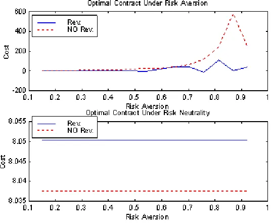
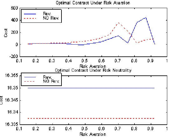
involving rewards awarded both after thefirst and second period. We display two graphs for each figure, one giving the contract cost under risk aversion as modeled in our paper, and the other giving the contract cost under risk neutrality as analyzed by LMP (2002).

Notice how for both the Original and the Extended repeated moral hazard models, the total wage costs for the optimal contracts under Revelation and No Revelation are not altered significantly by an increase in the parameterk. As shown in LMP (2002), the No Revelation contract remains consistently below that of the Revelation contract when the agent is risk neutral. However, once risk aversion is introduced in terms of the parameterσ, then we notice that in the Original Model whenE= 0.9(Figures 1-2), the cost of the No Revelation contract is consistently higher. More important is the fact that this difference is increasing rapidly as the degree of relative risk aversion increases especially afterσ= 0.5.

Figure 1: Original Model-k=0.75; E=0.9; U=5

Figure 2: Original Model-k=15; E=0.9; U=5

(exceedinge˜), the optimal Revelation contract calls for giving higher expected returns conditional onfirst period success compared to failure. With sufficient risk aversion, this might impose more risk on the agent when compared to the optimal No Revelation contract, which compensates the agent more following a failure due to the convexity ofh0_{(.)when σ >} 1

2. Hence, implementing a high

level of effort under significant risk aversion may reverse the results.

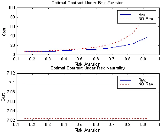
The Repeated Moral Hazard version of the model—shown in Figures 5-8— somewhat alters the results, depicting a convex path for the contract cost as a function of the relative risk aversion parameter. The No Revelation contract remains cheaper under risk neutrality as under the Original Model. However, as the agent becomes more and more risk averse, the cost of implementing the given amount of total effort rises at an increasing rate, with the cost difference between the No Revelation and Revelation contract also increasing substantially. When

kis increased however, the optimal contract cost is not significantly altered in either case.

Figure 3: Original Model-k=0.75; E=1.3; U=10

Figure 5: Extension of Model-k=0.75; E=0.9; U=5

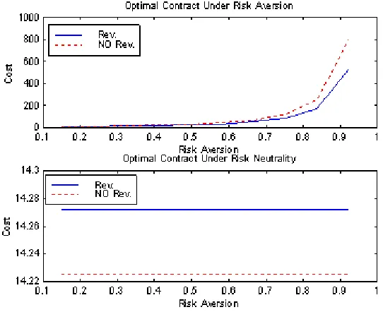
A reason why the Extended Model has higher contract costs under No Rev-elation for implementing a higher level of total effort when the agent is sub-stantially risk averse is that the principal now has an additional instrument he can use to insure the agent against risk: the rewards given conditional onfirst period outcomes, u1(s) and u1(f). Under the Original Model, implementing

a high level of first period effort necessitates that the agent bear substantial risk since it is optimal to provide greater expected second period returns fol-lowing a success compared to a failure. The Extended Model has potential to reduce this risk burden by providing intertemporal consumption smoothing using higherfirst period rewards following success. This in turn enables the op-timal Revelation contract to be less costly even when implementing high levels of effort.

Figure 8: Extension of Model-k=15; E=1.3; U=10

6

Conclusion

The question of providing uninformed agents with interim performance evalu-ations has recently been addressed by Lizzeri, Meyer and Persico (2002) under the assumption that the agent is risk neutral, and inefficiencies in the opti-mal contract arise due to limited liability on the part of the agent. Using a two-period, two-output dynamic principal-agent setting where the agent is compensated only after the second period, they are able to show that reveal-ing performance evaluations is able to generate a greater amount of effort from the agent given afixed incentive scheme. On the other hand, they also show that not revealing performance information to the agent enables the principal to implement a given amount of total effort at a strictly lower cost.

However, even when the principal is not forward looking enough, only to be concerned with the disutility he receives from the contract costs involved in implementing a given amount of effort the possibility of risk aversion on the part of the agent can be an important reason behind why information revelation can be optimal for the principal. The risk neutral agent is one who is in a better position to hedge himself against potential risk through other means, such as a student who takes multiple courses, therefore having his overall GPA depend on not a single one. For such a student the disutility from receiving a low grade on one course will not be so great, since she can make up for it through her other courses. However, once the agent is locked into a relationship with a single principal and is not informed, she is more likely to have a higher aversion towards the risk of getting a low grade. The principal may thenfind it optimal to share performance information in an attempt to reduce the disutility a risk averse agent may derive from uncertainty.

When this consideration is taken into account, we show that the results obtained by LMP (2002) can be significantly altered. First, for a given fixed reward mechanism, the optimal effort provided by the agent can be greater when no information is revealed compared to when it is. This may occur when the principalfinds it optimal to insure the agent by equating the expected rewards following a success to that following a failure, which usually occurs as the agent’s degree of risk aversion increases. Hence, when no information is revealed, if the agent is sufficiently risk averse, it will be optimal for the agent to insure himself by exerting more effort in the first period compared to when information is revealed. However, no comparison in total effort levels between the two scenarios can be made if the principalfinds it optimal to provide higher expected returns following an initial failure. That is when the agent is substantially risk averse, and the principal insures him by rewarding him by more following a failure, then the optimal second period effort under no information revelation will exceed that under information revelation while the reverse holds for the optimalfirst period effort.

Aside from the implications on the agent’s effort level, the optimal incentive scheme chosen by the principal can also exhibit alternative properties under the two scenarios. While the principal finds it optimal to only reward the most preferred outcome under no information revelation when the agent is risk neutral, he can no longer implement the same amount of effort using such a strong incentive mechanism once the agent is risk averse. The reason behind this is that the optimal contract when the agent is risk averse calls for a trade-offbetween incentive provision and insurance provision. Since the agent values consumption smoothing when risk averse, by providing incentives that are too strong, the principal will be forcing the agent to bear more risk than she is willing to. Hence, he chooses to optimally spread the rewards across the different possible outcomes thereby reducing incentives and risk at the same time.

of the responsibility for bearing the uncertainty regarding the second period outcome can be born by the agent. The principal is therefore using this op-portunity to spread incentives into the second period by implementing different effort levels depending onfirst period output. By so doing, he is actually diff er-entiating between the expected rewards following an initial success and a failure. Recall that, once we impose the additional constraint equatinge2(s)ande2(f),

we restrict the principal’s ability to do this, forcing him to bear all the risk for

first and second period performance, since he is not letting the agent adjust her effort against failure in the second period. This consumption smoothing effect reduces the incentive effect, implementing the same effort at greater cost.

We showed that this added restriction made the principal’s problem under information revelation equivalent to that under no information revelation when the derivative of the inverse utility function, h0_{(.) is linear. In fact, once it}

is relaxed, the principal may achieve a strictly better solution for the optimal contract at the margin by either increasing the expected reward following a failure if the first period effort implemented is low enough or increasing the expected reward following a success if the first period effort implemented is high enough. Alternatively, it is also optimal to raise the first period effort level implemented upon relaxing the constraint, while keeping the second period effort levelse2(s)ande2(f)fixed as before.

The computational results provided in section 5 support these theoretical

findings and extend them to show what happens to the optimal contract cost under the two scenarios once the derivative of the inverse utility function moves from being concave to being convex as the risk aversion parameter increases. The results show that for the original model considered, where the agent is only compensated after the second period, a given amount of total effort is always less costly to implement under information revelation when the total effort to be implemented is less than one. Otherwise, when implementing high levels of total effort, once the agent becomes highly risk averse, no information revelation becomes optimal. This can be explained by the fact that information revelation calls for implementing a high amount offirst period effort by increasing expected rewards conditional on success compared to failure. However, increasing the incentive provision effect in this way makes the agent bear more risk, which becomes more costly if the agent is substantially risk averse. The optimal no revelation contract on the other hand, calls for greater expected rewards conditional on failure when the agent is highly risk averse. If these rewards are high enough, they can still implement a total effort greater than one without imposing as much risk on the agent.

7

Appendix

In this Appendix we show the positivity of all the multipliers in the Revelation problem. First, we write thefirst order conditions of the principal’s problem with respect tou:

∂£R

∂u(s, s) : h

0_{(u(s, s)) =λ+}µ1

e1

+ µ2(s)

e1e2(s)

(12)

∂£R

∂u(s, f) : h

0_{(u(s, f)) =λ+}µ1

e1 −

µ₂(s)

e1(1−e2(s))

(13)

∂£R

∂u(f, s) : h

0_{(u(f, s)) =λ}

−₁µ1 −e1

+ µ2(f) (1₋e1)e2(f)

(14)

∂£R

∂u(f, f) : h

0_{(u(f, f)) =λ−} µ1

1₋e1 −

µ₂(f) (1₋e1)(1−e2(f))

(15)

Subtracting (13) from (12), and (15) from (14) we get:

h0(u(s, s))₋h0(u(s, f)) = µ2(s)

e1e2(s)(1−e2(s))

>0

⇒ µ₂(s)>0

h0(u(f, s))₋h0(u(f, f)) = µ2(f)

(1₋e1)e2(f)(1−e2(f))

>0

⇒ µ₂(f)>0

which shows that µ₂(s)and µ₂(f)are strictly positive sinceh0_{(.)is strictly}

increasing andu(s, s)6=u(s, f)and u(f, s)6=u(f, f). Using the positivity of

µ₂(s)andµ₂(f)along with the principal’sfirst order conditions with respect to effort we have:

∂$R

∂e2(s):e1[1−(h(u(s, s)−h(u(s, f)))]−µ2(s)c

00_(e

2(s)) = 0

∂$R

∂e2(f) : (1−e1)[1−(h(u(f, s))−h(u(f, f)))]−µ2(f)c

00_(e

2(f)) = 0

e1[1−(h(u(s, s)−h(u(s, f)))] = µ2(s)c00(e2(s))>0 (16)

(1−e1)[1−(h(u(f, s))−h(u(f, f)))] = µ2(f)c00(e2(f))>0 (17)

∂$R

+[1₋(h(u(s, f))₋h(u(f, f)))]₋µ₁c00_(e

1) = 0

⇒e2(s)[1−(h(u(s, s))−h(u(s, f)))]

| {z }

>0by (16)

+(1−e2(f))[1−(h(u(f, s))−h(u(f, f)))]

| {z }

>0by (17)

+

[h(u(f, s))₋h(u(s, f))] =µ₁c00_(e

1)

Subtracting (13) from (14) we also have:

h0(u(f, s))₋h0(u(s, f)) = −µ1

e1(1−e1)

+ µ2(f) (1₋e1)e2(f)

+ µ2(s)

e1(1−e2(s))

(18)

If µ_{1 ≤} 0 _⇒ h0_{(u(f, s))−h}0_{(u(s, f)) > 0 must necessarily hold by (18),}

and this impliesu(f, s)> u(s, f)_⇒h(u(f, s))₋h(u(s, f))>0_⇒µ₁c00_(e

1)>0,

which can be inferred from∂$R

∂e1 given above, which meansµ1>0⇒contradiction.

References

[1] Grossman, Sanford and Oliver Hart. (1983). “An analysis of the principal-agent problem”,Econometrica,51, 7-45.

[2] Laffont, Jean-Jacques and Martimort, David (2002). The Theory of Incentives-The Principal-Agent Model. Princeton and Oxford: Princeton University Press

[3] Lizzeri, Alessandro, Meyer, Margaret A. and Persico, Nicola. (2002). “The Incentive Effects of Interim Performance Evaluations”, CARESS Working Paper #02-09.

[4] Mirrlees, James. (1976). “The optimal structure of incentives and authority within an organization”,Bell Journal of Economics,7.

[5] Rogerson, William. (1985a). “The first-order approach to principal-agent problems”,Econometrica,53, 1357-1367.