A DFIM Sensor Faults Multi Model Diagnosis Approach Based on an Adaptive PI Multiobserver—Experimental Validation

http://dx.doi.org/10.4236/ijmnta.2015.42012

A DFIM Sensor Faults Multi-Model Diagnosis

Approach Based on an Adaptive PI

Multiobserver—Experimental Validation

Abid Aicha, Benhamed Mouna, Sbita Lassaad

National Engineering School of Gabes, Tunisia, Photovoltaic, Wind and Geothermal Systems Research, Gabes, Tunisia

Email: [email protected], [email protected], [email protected]

Received 19 April 2015; accepted 23 June 2015; published 30 June 2015 Copyright © 2015 by authors and Scientific Research Publishing Inc.

This work is licensed under the Creative Commons Attribution-NonCommercial International License (CC BY-NC).

http://creativecommons.org/licenses/by-nc/4.0/

Abstract

This paper studies the problem of diagnosis strategy for a doubly fed induction motor (DFIM) sensor faults. This strategy is based on unknown input proportional integral (PI) multiobserver. Thecontribution of this paper is on one hand the creation of a new DFIM model based on mul-ti-model approach and, on the other hand, the synthesis of an adaptive PI multi-observer. The DFIM Volt per Hertz drive system behaves as a nonlinear complex system. It consists of a DFIM powered through a controlled PWM Voltage Source Inverter (VSI). The need of a sensorless drive requires soft sensors such as estimators or observers. In particular, an adaptive Proportional-Integral mul-ti-observer is synthesized in order to estimate the DFIM’s outputs which are affected by different faults and to generate the different residual signals symptoms of sensor fault occurrence. The con-vergence of the estimation error is guaranteed by using the Lyapunov’s based theory. The proposed diagnosis approach is experimentally validated on a 1 kW Induction motor. Obtained simulation re-sults confirm that the adaptive PI multiobserver consent to accomplish the detection, isolation and fault identification tasks with high dynamic performances.

Keywords

Diagnosis, Doubly Fed Induction Motor, Multi-Model Approach, Adaptive PI Multi-Observer

1. Introduction

A. Aicha

rolling, rail traction or even marine propulsion or pumping. Nevertheless, it arrives that this machine presents an electric or mechanical defect.

In recent years, the development of fault diagnosis techniques has become an important issue seen the contin-uing evolution of modern systems complexity and the increasing demand for improving the reliability and secu-rity of controlled systems [1]-[5].

Observer-based diagnosis method is one of the wide variety of different diagnosis approaches that have al-ready been proposed in the literature, these approaches are based on the use of an adequate model [6]-[10]. It is often difficult to synthesize a sufficient model that is able to take into account the system’s nonlinearity and complexity. Thus many different approaches have been developed to deal with this problem. As a solution, mul-ti-model approach is one of the most widely used modeling techniques. This approach consists in representing the whole behavior of a nonlinear system by a set of simple local models. Generated sub models are then com-bined using validity function to contribute to the construction of the whole model [11]-[13]. Indeed, the multi- models facilitate the extension of some analysis tools that are developed in linear context to nonlinear context.

Then, faults diagnosis consists in the use of multiobserver based on decoupled multi-model structure [14]-[19]. Within this diagnosis context, the main objective of this paper is the detection and isolation of different types of sensor faults that may affect the doubly fed induction motor.

As it is the workhorse of industry, the use of the doubly fed induction machine (DFIM) in industrial applica-tions has grown impressively in recent years especially for variable speed applicaapplica-tions. Thus, an increasingly growing interest is given to the implementation of a supervision process to ensure a safe application of this ma-chine. As the DFIM is a nonlinear complex system that is subject of load disturbances, it is often difficult to synthesize a single model, therefore, a single observer that is able to detect and isolate the system’s faults. Thus the multi-model approach may be a solution to facilitate diagnosis task.

This paper treats the different steps for the study of the diagnosis of DFIM sensor faults based on multimodel approach. Starting with the decoupled multi-model modeling of the DFIM Volt per Hertz drive system which consists of a DFIM powered through a controlled PWM Voltage Source Inverter (VSI) in presence of load dis-turbances, next the design of an adaptive PI multi-observer that will be exploited finally for the faults detection. The adaptive PI multi-observer is synthesized after modification of the PI multi-observer in the case of variable faults. Finally, the proposed diagnosis approach is validated experimentally on an Induction motor.

Section 2 is dedicated to DFIM modeling in the dq synchronous reference frame. Section 3 deals with the DFIM modeling via decoupled multiple model approach respecting the different steps that lead to the realization of this task. In section 4 an adaptive PI multiobserver is synthesized to be used in section 5 for the detection and isolation of sensor faults that can affect the motor. Section 6 is an experimental validation of the proposed diag-nosis method on a squirrel cage induction motor.

Simulation and experimental results for the DFIM multi-model modeling and the implementation of the di-agnosis approach are performed by using the environment MATLAB/SIMULINK.

2. Classic DFIM Modeling

The DFIM Volt per Hertz drive system consists of a DFIM powered through the grid in stator side and a PWM inverter in the rotor side [1]-[4].

The mathematical model of the DFIM is presented here via the dq equations in the reference frame. The equations for the stator and rotor voltage can be written as (1)-(4).

( )

( )

( )

( )

( )

( )

( )

( )

( )

( )

( )

( )

( )

( )

( )

( )

d

d d

d d

d d

d

sd

sd s sd s sq

sq

sq s sq s sd

rd

rd r rd r rq

rq

rq r rq r rd

t

V t R i t w t

t t

V t R i t w t

t t

V t R i t w t

t t

V t R i t w t

t ϕ

ϕ

ϕ

ϕ

ϕ

ϕ

ϕ

ϕ



= + −

  

= + +

 

 _{= + −}

 

 _{= + +}



where

s r

w = +w w (2)

The flux equations can be expressed as

( )

( )

( )

( )

( )

( )

( )

( )

( )

( )

( )

( )

sd s sd sr rd

sq s sq sr rq

rd r rd sr sd

rq r rq sr sq

t L i t M i t

t L i t M i t

t L i t M i t

t L i t M i t

ϕ ϕ ϕ ϕ

= +

 

= +

 

= +



 _{= +}



(3)

The mechanic equation is described as

( )

_{( )}

d

d

t em t r

p t

J T f t T

t

w N

Ω 

= − Ω −

 

 = Ω 

(4)

A Simulink model is built using the Equations (1)-(4) and the DFIM parameters in Table 1.

The DFIM model is highly nonlinear since it contains product terms such as speed w with flux φd or φq, con-sequently with current id or iq. Thus to cope with this problem the multi-model approach is next suggested.

3. The DFIM Drive System Modeling via Decoupled Multi-Model Approach

The multi-model approach consists in representing the system’s behavior with a set of local linear models. Every local model or sub model contributes to this global representation via a validity function which takes its values in {0, 1}.

The DFIM Modeling with multi-model approach is executed through a sequence of four steps which are clus-ters estimation, structure identification, parametric identification and local models combination.

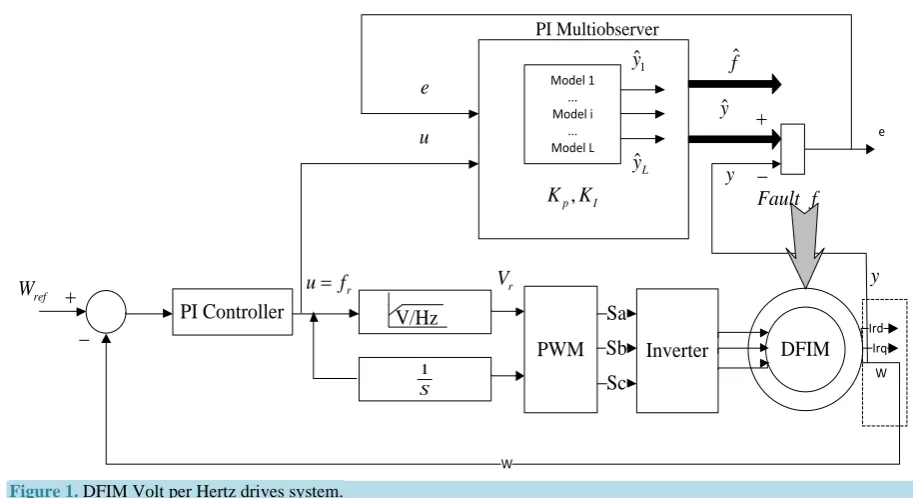
The performance of the cluster estimation depends on the quality of data base which must be rich in informa-tion. The process inputs and outputs are acquired after application of a voltage scalar control strategy as shown in

Figure 1.

An excitation produced by applying a variable amplitude high frequency signal at the desired speed loop. The acquisition phase consists in the collection of the DFIM’s output signals; the speed, the rotor currents ird and irq.

The rotor frequency fr is considered as the system’s input signal. The multi-model modeling is applied in such a way to create the system’s model in presence of load disturbances, thus a variable Load torque is produced by a pseudo random binary signal.

Next, the input-output collected data on DFIM are clustered into several groups through a Chui’s clustering

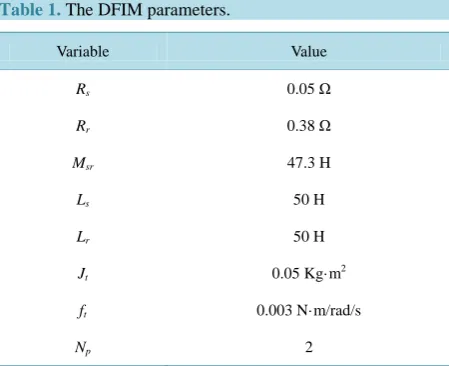
Table 1.The DFIM parameters.

Variable Value

Rs 0.05 Ω

Rr 0.38 Ω

Msr 47.3 H

Ls 50 H

Lr 50 H

Jt 0.05 Kg·m2

ft 0.003 N·m/rad/s

A. Aicha

Figure 1. DFIM Volt per Hertz drives system.

algorithm. Then, the structure identification is performed on each cluster using instrumental determinants ration (RDI) method or the general procedure for order estimation while the parameters identification of each sub model are identified using recursive least square (RLS) method. Finally, obtained sub models are combined using the validity concept.

The different steps of multi-model modeling and implementation are performed thanks to MATLAB/ SIMULINK environment

The modeling strategy leads to a decoupled multi-model with six sub models which can be presented as fol-lows.

(

)

( )

( )

( )

( )

( )

( ) ( )

1

1

i i i i i

i i i

L

i i

i

x k A x k B u k D

y k C x k

y k V k y k

=



 _{+ = + +}

 ₌

 

 ₌



∑

(5)

ni i

x ∈ , yi∈p and u are respectively the system’s i

th

state, output and input. Where ni = 3, p = 3.

, 1, , 6

i i

i i rd rq

i i

x w i i i

u fr

y x

 _{= }′ ₌

  

 =   =  



(6)

Vi is the ith validity value which computes the ith sub model’s contribution to the creation of the system’s glob-al output. These functions have the following properties (7).

( )

( )

{

}

1

1

0 1 1, 2, ,

N i i

i V k

V k i N

=

 ₌

 

 ≤ ≤ ∀ ∈



∑



(7)

The different obtained DFIM system’s matrixes are expressed as (8)-(11). PI Controller

PWM Inverter

1

S

DFIM

W

V/Hz ref

W u= fr Vr

Sc Sa

Sb

y

+

− Ird_Irq

W Model 1

... Model i

... Model L PI Multiobserver

1

ˆ

y

ˆ_L

y

ˆ

y ₊

−

e

y e

u

ˆ

f

, p I

1 2

3 4

5 6

0.982 0 0 0.990 0 0

0 0.970 0 , 0 0.946 0 ,

0 0 0.941 0 0 0.960

0.977 0 0 0.989 0 0

0 0.945 0 , 0 0.957 0 ,

0 0 0.982 0 0 0.968

0.976 0 0 0.999 0 0

0 0.986 0 , 0 0.990 0

0 0 0.959 0 0 0.966

A A

A A

A A

   

   

=_ − _ =_{ }

   

   

   

   

=_{ } =_{ }

   

   

 

 

=_{ } =

 

 

 

 

 

 

 

(8)

1 2 3

4 5 6

0.025 0.081 0.057

0.011 , 0.029 , 0.019 ,

0.070 0.095 0.135

0.012 0.057 0.034

0.004 , 0.016 , 0.001

0.056 0.079 0.067

B B B

B B B

     

     

=_{ } =_{ } = −_{ }

     

     

     

     

= −_{ } =_{ } =_{ }

     

     

(9)

1 2 3 4 5 6 1

1 0 0

0 1 0 ,

0 0 1

C C C C C C C

 

 

=_{ } = = = = =

 

 

(10)

1 2 3

4 5 6

0.048 1.085 0.751

0.911 , 4.690 , 3.738 ,

1.678 2.331 0.856

0.550 4.319 0

5.323 , 2.263 , 0.025

3.188 3.662 0.064

D D D

D D D

−

     

     

=_{ } =_{ } =_{ }

    − 

     

−

     

     

=_{ } =_{ } =_{ }

  −   

     

(11)

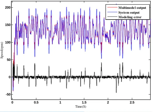
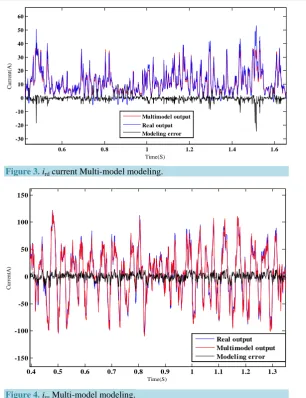
By exciting the system with a variable input, the modeling results of the speed, the current ird and the current irq are shown in Figures 2-4. We can notice that the multi-model outputs follow with acceptable error the real

outputs.

Figure 2.Speed Multi-model modeling.

0 0.5 1 1.5 2 2.5

-50 0 50 100 150 200

Time(S)

S

pe

e

d(

rpm

)

A. Aicha

Figure 3. ird current Multi-model modeling.

Figure 4. irq Multi-model modeling.

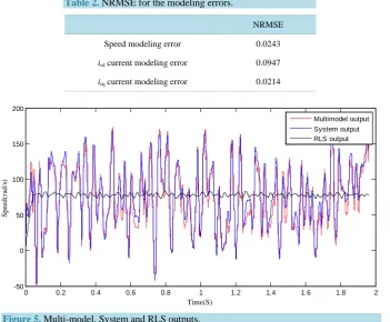
The normalized roots mean square modeling error NRMSE for each modeling error; the speed, ird and irq

modeling error are calculated and given inTable 2.

The obtained multi-model is compared to a model done by RLS method, Figure 5 approves the efficiency of the multi-model.

Next this multi-model will be exploited in the multiobserver design.

4. Adaptive Proportional-Integral Multiobserver Designs

In this section we propose to study in the first part the PI multiobserver then the modified or adaptive PI mul-tiobserver in second part of this section.

Firstly, the DFIM decoupled multi-model structure is modified in order to take into account the unknown in-put vector, and then exploited in the rest of this paper in order to conceive the based observer diagnosis’s strate-gy.

(

)

( )

( )

( )

( )

( )

( )

( )

( ) ( )

1

1

i i i i i i

i i i

N

i i

i

x k A x k B u k D E f k

y k C x k Mf k

y k V k y k

=



 _{+ = + + +}

 _{= +}

 

 ₌



∑

(12)

0.6 0.8 1 1.2 1.4 1.6

-30 -20 -10 0 10 20 30 40 50 60

Time(S)

C

u

rre

n

t(A

)

Multimodel output Real output Modeling error

0.4 0.5 0.6 0.7 0.8 0.9 1 1.1 1.2 1.3

-150 -100 -50 0 50 100 150

Time(S)

C

ur

re

nt

A

)

Table 2. NRMSE for the modeling errors.

NRMSE

Speed modeling error 0.0243

ird current modeling error 0.0947

irq current modeling error 0.0214

Figure 5. Multi-model, System and RLS outputs.

where Ei and f identify, respectively, the impact of the unknown input on the state’s system and the unknown input vector.

4.1. PI Multiobserver

The PI structure is developed below in favor of achieving simultaneously estimation of both state and unknown inputs.

(

)

( )

( )

( )

(

( ) ( )

)

(

)

( )

( )

(

( ) ( )

)

( )

( )

( )

( )

1

1

ˆ _ˆ

1

ˆ 1

ˆ

i i i i i i pi

N

i I

i N

i i i i

x k A x k B u k D E f k K y k y k

f k f k V k K y k y k

y k V k C x k Mf k

=

= 

 + = + + + + −

 

+ = + −

  

= +

 

∑

∑

(13)

where xi and y denote respectively the estimated state vector and output vector. Vi are the validities functions calculated in the modeling phase.

This observer is known as a robust observer regarding the unknown inputs that have feebly variation. The main task of the observer design is to find out the gain matrices KI and Kpi.

The PI observer uses the influence of the rebuilding output’s error with a proportional effect to estimate the system’s whereas the integral effect is used to estimate the signal of sensor or actuator’s defaults.

The sub models’ outputs yi(k), used, as modeling’s artificial signals, to represent the real system’s behavior are not exploitable to control an observer, indeed only the multi-model’s total output y(k) as it is accessible to mea-surement, can be designed with a system’s physical quantity. Thus an augmented system is defined below.

(

)

( )

( )

( )

( )

( ) ( )

( )

1

x k Ax k Bu k D Ef k

y k C k x k Mf k

 + = + + +

 

= +



   

 



  (14)

0 0.2 0.4 0.6 0.8 1 1.2 1.4 1.6 1.8 2

-50 0 50 100 150 200

Time(S)

S

p

eed

(r

ad

/s

)

A. Aicha

where

( )

( )

( )

( )

1

, N n

i N i

i

x t x t x t x t R n n

=

 

=_{ } ∈ =

∑

   (15)

{

}

( )

( )

[

]

0 0 ,

, , , , , n n N n m N N p n i i i i i n l N n l N

A diag A A R

B B B R

C k V k C R

C C

D D D R

E E E R

× × × = × ×  = ∈   =_ _ ∈   = ∈    =   _{=  ∈}     _{=  ∈}    

∑

By the use of the Lyapunov’s approach defined below and taken advantage of ensuring the employed observ-er’s stability, and in order to guarantee the convergence of the estimation’s error, the conditions generated in forms of linear matrix inequalities (LMI) permit to compute the observer’s gains. Thus the following theorem proposed in [14] [15] suggests sufficient conditions ensuring the exponential convergence of the estimation’s error.

Theorem: The estimation error between the decoupled multi-model (12) and the PI observer (13) converges

exponentially towards zero if there exists a symmetric definite positive matrix P and a matrix G verifying the LMI following:

(

)

2 1

0, 1, ,

i a

i a

P C G A P

i N

GC PA P

α

 − − 

< =

 

− −

   (17)

where

( )

( )

, 0

a i i

A E

A C t C t M

I     =_{ } =_{ }     _ (18)

α is the attenuation rate which serves to quantify the convergence speed of the estimation error. Having 0 < α < 0.5 let to find the KI and Kp gains as:

1

a

K =P G− (19)

The state’s estimation e and input’s estimation errors ԑ are given by the following equation:

( )

( ) ( )

( )

( )

( )

ˆ

ˆ

e k x k x k

t f k f k

ε  = −   = −    (20)

Taking into account the fact that the unknown inputs are considered as constant or with very slow dynamics,

(

)

( )

f k+ − f k ≈ (21)

Then

(

)

(

)

( )

( )

( )

( )

e k A K C k E K M e k

k K C k I K M k

ε ε    +  − −   =    ₊  _{− −}              

 (22)

Considering the definition of augmented system, the augmented error can be defined as

(

)

(

( )

)

( )

a a a a a

where

( )

( )

_{( )}

T

T T

1, ,

a

P a

I

P P PN

e k e k k K K K

K K K

ε    =        _{ }  ₌          =  _{ }    _ (24)

The Lyapunov approach is defined as

( )

(

)

( ) ( )

, 0

V e k =e k Pe k P> P=P (25)

The exponential convergence is guaranteed if there exists a symmetric definite positive matrix P and a posi-tive scalar α verifying the following condition:

( )

(

)

(

( )

)

V e k

α

∆ + < (26)

With

( )

(

)

(

(

)

)

(

( )

)

V e k V e k V e k

∆ = + − (27)

This PI multiobserver is studied and developed by [17] [18], however, the studied multiobserver is valid only in the case of slowly varying faults.

4.2. Adaptive PI Multiobserver

To consider the case of variable fault, as expressed in (28), we propose to create an adaptive PI multiobserver that is based on the updating of the estimated validity functions ˆVi which are computed as the Equations (29)- (31).

In fact the real system depends on the fault, so the multiobserver design should also consider this fault therefore in each instant a new validities are computed in order to guarantee always the convergence of the resi-due ri expressed by (29).

(

)

( )

f k+ − f k ≠ (28)

( )

( )

( )

i i

r k = y k −y k (29)

Then simple validities are expressed by (30).

( )

( )

( )

∑

The final adaptive validities after normalization and reinforcement of the simple validities functions are ex-pressed in (31).

( )

( )

( )

j j i

i

r k N

N

i

i j j i

A. Aicha

The Final adaptive PI multiobserver is developed in (32).

(

)

( )

( )

( )

(

( ) ( )

)

(

)

( )

( )

(

( ) ( )

)

( )

( )

( )

i i i i i i pi

N

i I

i N

i i i i

x k A x k B u k D E f k K y k y k

f k f k V k K y k y k

y k V C x k Mf k

= =   + = + + + + −   + = + −    = +  

∑

∑

5. Detection and Isolation of DFIM System’s Sensors Faults

In this section, the main task to be reached is detection and isolation of the Doubly fed Induction motor’s faults by means of a designed adaptive PI multi-observer synthesized to estimate the different system outputs. Within this part the fault effect on the system state is expressed with Ei, i = 1,···, N while M represents the faults effect on the DFIM output.

Three types of sensor faults are considered, they affect respectively the speed Ω, the ird current and the irq

cur-rent. The faults are variable and have sinus form.

The PI multiobserver structure is equivalent to a bank of three multiobservers since

ˆ

ˆ _{rd rq}

y= Ω_ i i _ (33)

The different faults are chosen to be occurred in the same date. In this case;

0.2 0 0

0 0.2 0

0 0 0.2

M     =       (34) And

0, 1, ,

i

E = ∀ =i  N (35) The resolution of the different LMI helps to find the matrices gains then to construct the PI multiobserver. The

KPi and KI gains are given by (36).

1 2 3

4 5 6

0.121 0 0 0.123 0 0 0.120 0 0

0 0.057 0 , 0 0.115 0 , 0 0.115 0 ,

0 0 0.114 0 0 0.118 0 0 0.122

0.123 0 0 0.120 0 0 0.273 0 0

0 0.118 0 , 0 0.124 0 , 0 0.277 0

0 0 0.120 0 0 0.118 0

p p p

p p p

K K K

K K K

            =_ − _ =_{ } =_{ }                     =_{ } =_{ } =         , 0 0.274

0.134 0 0

0 0.127 0

0 0 0.131

I K               =       (36)

The residual equations are given as follows:

1 1 2 2 3 3 ˆ ˆ ˆ s id iq

R y y

R y y

R y y

 = −  _{= −}   _{= −}  (37)

ˆ_i

y designate the ith estimated output and yi designate the ith real system output in no faulty case.

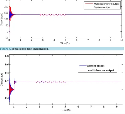
Obtained results approve the performance of the fault estimation method; the different system’s outputs yi, i = 1, ···, 3 follow rapidly and respectively, the real ones yi with satisfied error as shown in Figure 6, Figure 7 and

Figure 8.

The different fault evolutions approve that the estimated fault is occurred at the same time when the real fault is occurred so the detection task is verified.

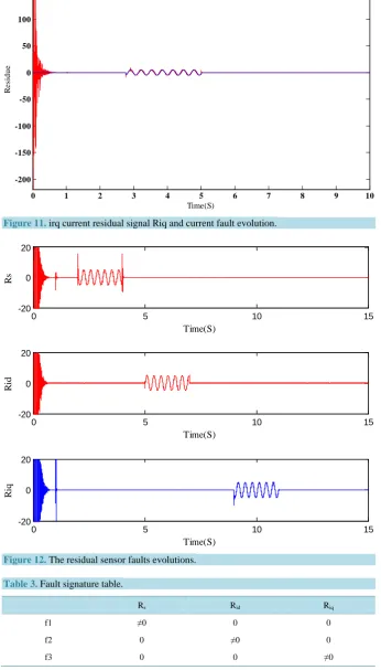
The three residual signals shown in Figure 9, Figure 10 and Figure 11 follow with high precision the differ-ent sensors fault signals and approve that the faults are well iddiffer-entified.

The isolation task is verified since for each system output a multiobserver is synthesized, i.e. each residue is sensitive to only one sensor fault and insensitive to all other faults concerning the residual signals computed in (36).

The isolation of the different sensor faults can be summarized in the Figure 12. In fact, if a speed sensor fault f1 is occurred then the residual signal Rs ≠ 0, if an ird current sensor fault f2 is occurred then the residual signal

Rid ≠ 0, and if an irq current sensor fault f3 is occurred, the residual signal Riq ≠ 0.

Considering the previous results, generated relationship can be described in a summarized table as shown in

Table 3.

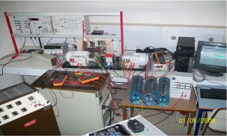
6. Experimental Validation

In this section the proposed diagnosis approach is validated experimentally on 1 KW squirrel cage Induction motor.

Figure 6. Speed sensor fault identification.

Figure 7. ird current sensor fault identification.

0 1 2 3 4 5 6 7 8 9 10

-50 0 50 100 150 200 250

Time(S)

S

pe

ed (

rpm

)

Multiobserver PI output

System output

1 2 3 4 5 6 7 8 9

-0.2 0 0.2 0.4 0.6 0.8

Time(S)

C

u

rre

n

t (A

)

System output

A. Aicha

Figure 8.irq current sensor fault identification.

Figure 9. Speed residual signal Rs and speed sensor fault evolution.

Figure 10.ird current residual signal Rid and current fault evolution.

1 2 3 4 5 6 7 8

-6 -4 -2 0 2 4 6 8 10

Time(S)

C

u

rre

n

t(A

)

Estimated current irq System current irq

0 1 2 3 4 5 6 7 8 9 10

-40 -20 0 20 40 60 80 100

Time(S)

R

es

idue

1 2 3 4 5 6 7 8 9

-10 -5 0 5

Time(S)

R

e

si

Figure 11.irq current residual signal Riq and current fault evolution.

Figure 12. The residual sensor faults evolutions.

Table 3. Fault signature table.

Rs Rid Riq

f1 ≠0 0 0

f2 0 ≠0 0

f3 0 0 ≠0

0 1 2 3 4 5 6 7 8 9 10

-200 -150 -100 -50 0 50 100 150

Time(S)

R

e

si

due

0 5 10 15

-20 0 20

Time(S)

Rs

0 5 10 15

-20 0 20

Time(S)

Ri

d

0 5 10 15

-20 0 20

Time(S)

Ri

A. Aicha

An experimental set up drive system exposed in Figure 13 is prepared to provide a set of input/output mea-surement with the help of MATLAB/SIMULINK and DSpace system with DS1104 controller board based on the digital signal processor (DSP) TMS320F240. The measurement of the stator current is achieved via Hall type sensors. An incremental encoder position sensor delivering 1024 pulses per revolution is used to detect The IM speed. Load torque is generated by a resistive bank fed by a DC generator.

To create parameter variation we propose to use a variable resistor that is connected in series to each phase of the motor to vary the stator resistance

The experimental set up is exploited to collect a rich database at 600 rpm with a wide range of loads and sta-tor resistance variations.

The database is then clustered into eight clusters. Next a structural and parametric identification is performed into the obtained cluster to generate the eight local models. Finally a multi-model is created after the combina-tion of the local models pondered by validities funccombina-tions.

The obtained multi-model is next necessary to synthesize the adaptive PI multiobserver.

The resolution of the different LMI conditions helps to calculate the multiobserver gain matrices that are ex-pressed in Equation (38).

1 2 3

4 5 6

0.121 0.0340

0.113 0.0348 0.130 0.0376

, , 0.025 0.0200 ,

0.048 0.1184 0.046 0.1183

0.026 0.0208

0.025 0.0200 0

0.148 0.0354

0.085 0.0679 , ,

0.057 0.0813 0.047 0.1123

I I I

I I I

K K K

K K K

 

    _{ }

=_{ } =_{ } =_{ }

    _{ }

 

 

 

 

=_{ } =_{ } =

 

 

 

7 8

.063 0.0503 0.025 0.0200 , 0.043 0.0349

0.025 0.0200 0.025 0.0200

0.072 0.0575 , 0.071 0.0572

0.047 0.1096 0.047 0.0376

0.025 0

0 0.020

I I

p

K K

K

 

 

 

 

 

   

   

=_{ } =_{ }

   

   

 

=  

 

(38)

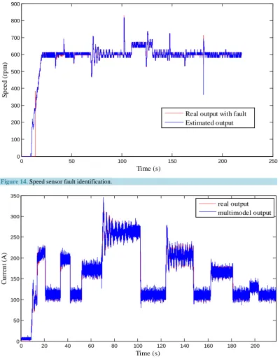
To test the obtained multiobserver, we inject two sensor fault, the first affect the speed sensor between t = 109 s and t = 130 s, while the second affect the current sensor between t = 14 s and 21 s.

Figure 14 and Figure 15 approve that the estimated speed and current signals follow the real ones affected with the faults. Figure 16 and Figure 17 expose the residual signals that approve that the estimated fault follow the real ones.

According to experimental results, we can resume that the detection of the sensor fault is successfully achieved. We can notice that the value of the residual signals (speed and current residue) changes from zeros only when the fault occurs.

The identification of the faults is approved as the two residual signals follow with high precision of the two sensors fault signals.

Figure 14. Speed sensor fault identification.

Figure 15.Is current sensor fault identification: Real current with fault and estimated current.

0 50 100 150 200 250

0 100 200 300 400 500 600 700 800 900

Time (s)

S

pe

e

d (

rpm

)

Real output with fault Estimated output

0 20 40 60 80 100 120 140 160 180 200

0 50 100 150 200 250 300 350

Time (s)

C

u

rre

n

t (A

)

A. Aicha

Figure 16. Speed residual signal Rw and speed sensor fault evolution.

Figure 17.Current residual signal Ris and current sensor fault evolution.

The fault isolation is proved as for each system output an estimated output is generated. Each residue is sensi-tive to only one sensor fault.

7. Conclusions

In this paper, a multi-model diagnosis strategy is applied to the detection and isolation of the different sensor faults that can affect the induction machine. Firstly the system’s modeling is investigated through the multi-

0 50 100 150 200 250

-3 -2 -1 0 1 2 3

Time (s)

S

peed (

rpm

)

Estimated fault Real fault

0 50 100 150 200 250

-0.8 -0.6 -0.4 -0.2 0 0.2 0.4 0.6 0.8 1 1.2

Time(S)

C

u

rre

n

t (A

)

Estimated fault

model approach. Then considering the system’s decoupled multi-model structure an adaptive PI multi-observer is synthesized. The novel multiobserver is synthesized exploiting the classic PI multiobserver that is modified to obtain the adaptive one. The modification consists in the multiobserver validities calculation. This multiob- server is used in the fault detection and isolation of the different sensor faults that can affect the system’s outputs. The obtained experimental and simulation results performed under MATLAB/SIMULINK environment show that the applied method has an excellent capacity to describe the Induction machine under faulty case. The ob-jectives are reached since the different computed residuals signals affirm that the detection, identification and isolation of the sensors faults are well achieved. In this paper the study is limited on simulation and without con-sidering actuators and system faults, thus, in future work experimental study concern the induction motor, in fu-ture work we will propose to validate experimentally the diagnosis approach on a DFIM under sensor and actu-ator faults.

Acknowledgements

This work was supported by grants from National Engineering School of Gabes, Tunisia, Photovoltaic, Wind and Geothermal Systems Research Unit, Gabes, Tunisia

References

[1] Gritli, Y., Stefani, A., Rossi, C., Filippetti, F. and Chatti, A. (2011) Experimental Validation of Doubly Fed Induction Machine Electrical Faults Diagnosis under Time-Varying Conditions. Electric Power Systems Research, 81, 751-766.

http://dx.doi.org/10.1016/j.epsr.2010.11.004

[2] Djeghali, N., Ghanes, M., Djennoune, S. and Barbot, J.P. (2013) Sensorless Fault Tolerant Control for Induction Mo-tors. International Journal of Control, Automation, and Systems, 11, 563-576.

http://dx.doi.org/10.1007/s12555-012-9224-z

[3] Saha, S., Aldeen, M. and Tan, C.P. (2011) Fault Detection in Transmission Networks of Power Systems. International Journal of Electrical Power & Energy Systems, 33, 887-900. http://dx.doi.org/10.1016/j.ijepes.2010.12.026

[4] Chen, J.H., Li, H.K., Sheng, D.R. and Li, W. (2015) A Hybrid Data-Driven Modeling Method on Sensor Condition Monitoring and Fault Diagnosis for Power Plants. International Journal of Electrical Power & Energy Systems, 71, 274-284. http://dx.doi.org/10.1016/j.ijepes.2015.03.012

[5] Darouach, M. (2012) On the Functional Observers for Linear Descriptor Systems. Systems & Control Letters, 61, 427-434. http://dx.doi.org/10.1016/j.sysconle.2012.01.006

[6] Manuja, S., Narasimhan, S. and Patwardhan, S.C. (2009) Unknown Input Modeling and Robust Fault Diagnosis Using Black Box Observers. Journal of Process Control, 19, 25-37. http://dx.doi.org/10.1016/j.jprocont.2008.02.004

[7] Pertew, A.M., Marquez H.J. and Zhao, Q. (2005) H∞ Synthesis of Unknown Input Observers for Non-Linear Lipschitz Systems. International Journal of Control, 78, 1155-1165. http://dx.doi.org/10.1080/00207170500155488

[8] Fu, Y.P., Cheng, Y.H. and Jiang, B. (2010) Robust Actuator Fault Estimation for Satellite Control System via Fuzzy Proportional Multiple-integral Observer Method. Proceedings of the 29th Chinese Control Conference, Beijing, 29-31 July 2010, 3942-3946.

[9] Sören, G. and Horst, S. (2014) Diagnosis of Actuator Parameter Faults in Wind Turbines Using a Takagi-Sugeno Slid-ing Mode Observer. Intelligent Systems in Technical and Medical Diagnostics, Advances in Intelligent Systems and Computing, 230, 29-40.

[10] Yang, X.-B., Jin, X.-Q., Du, Z.-M., Zhu, Y.-H. and Guo, Y.-B. (2013) A Hybrid Model-Based Fault Detection Strategy for Air Handling Unit Sensors. Energy and Buildings, 57, 132-143. http://dx.doi.org/10.1016/j.enbuild.2012.10.048

[11] Abid, A., BenHamed, M. and Sbita, L. (2011) Induction Motor Real Time Application of Multimodel Modeling Ap-proach. International Review of Electrical Engineering, 6, 655-660.

[12] Capron, B.D.O. and Odloak, D. (2013) LMI-Based Multi-Model Predictive Control of an Industrial C3/C4 Splitter.

Journal of Control, Automation and Electrical Systems, 24, 420-429. http://dx.doi.org/10.1007/s40313-013-0050-1

[13] Elfelly, N., Dieulot, J.Y. and Borne, P. (2008) A Neural Approach of Multimodel Representation of Complex Pro- cesses. International Journal of Computers, Communications & Control, 3, 149-160.

[14] He, S.P. (2014) Fault Estimation for T-S Fuzzy Markovian Jumping Systems Based on the Adaptive Observer. Inter-national Journal of Control, Automation and Systems, 12, 977-985. http://dx.doi.org/10.1007/s12555-013-0350-z

[15] Yu, C.H. and Choi, J.W. (2014) Interacting Multiple Model Filter-Based Distributed Target Tracking Algorithm in Underwater Wireless Sensor Networks. International Journal of Control, Automation and Systems, 12, 618-627.

A. Aicha

[16] Ichalal, D. (2009) Estimation et diagnostic de systèmes non linéaires décrits par un modèle de Takagi-Sugeno. PhD Thesis, Institut National Polytechnique de Lorraine, Nancy.

[17] Orjuela, R., Marx, B., Ragot, J. and Maquin, D. (2010) Fault Diagnosis for Nonlinear Systems Represented by Hetero-geneous Multiple Models. 2010 Conference on Control and Fault Tolerant Systems, Nice, 6-8 October 2010, 600-605.

http://dx.doi.org/10.1109/SYSTOL.2010.5675969

[18] Hamdi, H., Rodrigues, M., Mechmeche, C., Theilliol, D. and Benhadj Braiek, N. (2012) Fault Detection and Isolation in Linear Parameter-Varying Descriptor Systems via Proportional Integral Observer. International Journal of Adaptive Control and Signal Processing, 26, 224-240. http://dx.doi.org/10.1002/acs.1260