Low Complexity and High Quality Image Compression Algorithm for Onboard Satellite

Low-Complexity and High-Quality Image Compression

Algorithm for Onboard Satellite

Sujata Swamy

R.N.S.I.T Bangalore, Karnataka India

Mamatha A.S

R.N.S.I.T Bangalore, Karnataka India

Vipula Singh

Professor of ECE Department R.N.S.I.T Bangalore,

Karnataka India

ABSTRACT

Image Compression reduces redundancy in data representation in order to achieve saving in the cost of storage and transmission. Image compression compensates for the limited on-board resources, in terms of mass memory and downlink bandwidth and thus it provides a solution to the “bandwidth vs. data volume” dilemma of modern spacecraft. Thus compression is very important feature in payload image processing units of many satellites. A low complexity and high efficiency near-lossless image compression algorithm is suggested in this paper. The algorithm provides the average compression ratio of 1.403 with high image quality for lossless compression. Compression ratio increases as ∆ parameter increases. Using proposed algorithm compression ratio of 4.208 is achieved for near-lossless compression. The proposed algorithm has low memory cost suitable for hardware implementation.

General Terms

Image processing, Image compression, Near lossless compression algorithm.

Keywords

Satellite image compression, Near lossless image compression, Context modeling and Predictive coding, Pre-processing.

1.

INTRODUCTION

Most of the satellites operate on a store-and-forward mechanism. With the increase of spatial resolution and swath, the space missions are faced with the necessity of handling an extensive amount of imaging data. A digital image obtained by sampling and quantizing a continuous tone picture requires an enormous storage. For instance, a 24 bit colour image with 512x512 pixels will occupy 768 Kbytes storage on a disk and without compression only 911 such pictures can fit in a single compact disc. To transmit such an image over a 28.8 Kbps, modem would take almost 4 minutes.

Image compression [1] is a process of reducing the amount of data required to represent a digital image by removing redundant data. The image compression is used to reduce the storage requirement of a fixed memory system and decrease the time needed for transferring image data using lesser bandwidth. Efficient compression algorithms are developed for this and compression ratio (CR) is one of important parameter in determining efficient compression algorithm. Redundancy is the number of bits used to transmit a message minus the number of bits of actual information in the message. The number of bits actually required to represent the information in an image may be substantially less because of redundancy. For example if one representation of data takes

bytes and another representation of same data takes

bytes ( ), then is redundant. There are different types of redundancy present in an image, such as Spatial Redundancy, Statistical Redundancy and Human Vision Redundancy (HVR) [2].

In Spatial Redundancy the elements that are duplicated in a structure such as pixel in a still image and the current pixel information can be partially deduced by the neighboring pixels. Prediction or Transformation methods are used to remove these spatial redundancies. Statistical Redundancy occurs due to the fact that pixels within an image tend to have very similar intensities as those of its neighborhood, except at the object boundaries or illumination changes. It explores the probability of symbols. Here short codeword is assigned to high-probability symbols, and long codeword is assigned to low-probability symbols. Two popular methods which are used to remove the statistical redundancy are Huffman or Arithmetic coding. Many experiments have proven that the human eye does not respond with equal sensitivity to all incoming visual information or to higher frequency components. Removing such type of redundancy (HVR) is normally achieved by Quantization, with high-frequency elements being over quantized or even deleted.

There are different techniques for compressing images. These are broadly classified into three classescalled lossless, lossy and near-lossless compression techniques. Lossy technique causes image quality degradation in each compression or decompression step. In general, lossy techniques provide for greater compression ratios than lossless techniques. Lossy compression does not allow the exact original data to be reconstructed from the compressed data, where as in lossless image compression reconstructed image is exactly same as the original image. Lossless compression methods are generally used in medical imaging, satellite imaging or any other area where data loss cannot be permitted. Lossy methods are most often used for compressing sound, images or videos in multimedia applications, video conferencing, broadcast TV etc. Near-lossless compression is a lossy compression method where the reconstructed pixels differ from the original pixels by no more than a predetermined value. In near-lossless compression data is guaranteed to be within a specified range based on the near-lossless threshold. In this paper, we have proposed image compression algorithm suitable for onboard satellite. Contents of the paper include the following sections. Analysis of some previous lossless image compression techniques are presented in the section II. Section III contains the details of actual implementation of the design in depth. In section IV, the results of this design have been discussed. Section V has concluding remarks.

2.

IMAGE COMPRESSION

encoded image without loss of information, lossless compression is widely used and it gives moderate compression ratio. Lossless image compression is well established as a means of reducing the volume of image data from deep space missions without compromising the data quality. Missions often desire hardware to perform such compression [3], in order to reduce the demand on spacecraft processors and to increase the speed at which images can be compressed.

There are different lossless compression techniques proposed by different authors, which gives benefits in terms of higher compression, high throughput, high speed and low power consumption. Guoxia Yu.et al. [4] have proposed a lossless image compression scheme which is a combination of 2-D Prediction and Independency-coding. It makes use of Vertical Scan which goes down vertically, and turns from the start again after N pixels. Guoxia’s method achieves high compression ratio around 93%. Jose Luis Nunez [5] used Dynamic modeling approach which gives higher compression ratio than that of Consultative Committee for Space Data Systems (CCSDS). This dynamic modeling is specialized to each data type such as general data, image data and multi-spectral or video data and it uses combination of Context modeling and Predictive coding. Yanez Raffaele Pizzolante [6] used another low complexity, Spectral oriented Least Square (SLSQ) algorithm. The concept of distance is used in SLSQ which gives good compression ratio around 3.21 where as Jun Takada’s [7] method is based on FELICS, which is simple, hierarchical predictive coding method and achieves 7-35 times faster compression than existing methods such as JPEG2000. This provides a significant performance increase (50% faster compression in most cases), with only a slight decline in estimation accuracy (0.5% decline in compression ratios). Ze Wang’s [8] Pipelined architecture scheme is good for high-speed compression of satellite remote sensing image onboard satellite. This design achieves much lower complexity and super high data throughput through an improved prediction model by breaking the feedback loop of context parameters updating. The processing speed of this design is up to 75Mpixels per second, while the compression ratio is slightly lower than the standard JPEG-LS compression. Cheng-Chen Lin’s [9] algorithm uses two-stage predictor and an entropy coding module which gives the advantages in terms of compression efficiency and memory usage. The stage-1 supports both intra (spatial) and inter-band (spectral) predictions. The prediction resulted from the stage-1 predictor acts as an initial value to the stage-2 predictor. Based on the requirements these techniques can be used in the applications.

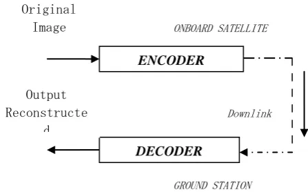
General block diagram of image compression system onboard satellite is shown in fig.1, where compression algorithm compresses the images which are captured by camera of the satellite. This system produces compressed data and using one of the efficient entropy coding techniques the compressed data is then encoded into bit stream, which is then sent over the

downlink to ground station. This compression system should consume lesser onboard power, area and bandwidth.

Figure 1: General block diagram of onboard image compression

The compression algorithm should be designed in such a way that it should not only increase the compression ratio, but it should also reduce the complexity. This paper presents a new compression technique which enhances the compression ratio and reduces the complexity.

3.

PROPOSED ALGORITHM

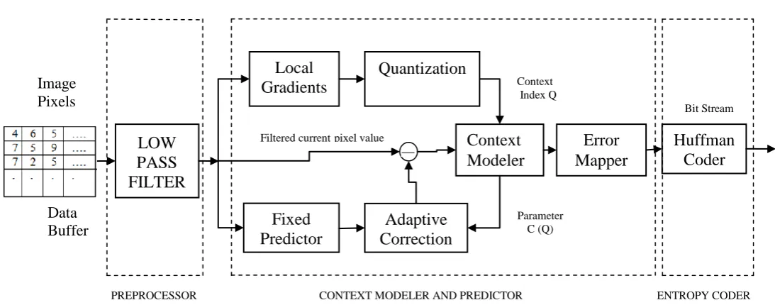
A modification to JPEG-LS algorithm is proposed here by adding a Pre-processor block before context modeler and predictor block. General block diagram of the proposed algorithm is as shown in fig.2. The encoder has mainly 3 blocks Pre-processor, Context modeler and predictor, Entropy coder. The image pixel values are directly given to pre-processor block. Output of pre-pre-processor is losslessly compressed by context modeler and predictor. Adding pre-processor block further increases the compression ratio thus giving good performance. Huffman coding is used as entropy coder where the encoded bit-stream from huffman encoder is stored or transmitted over downlink. Decoder is reverse process of encoder.

3.1

Pre-Processor

In the pre-processing block as shown in fig.3, a low pass filter is used. This method [10] has been applied in the wireless endoscopic capsule to reduce the communication bandwidth and transmitting power of image data. In the proposed method, the image data is first low-pass filtered and then compressed by a lossless image compression coder that is context modeler and predictor. It has a very low complexity hardware implementation. A simple structure of the pre-processor method is illustrated by the smoothing operation as shown in fig.4. All the pixels except those in the first row are filtered row by row as illustrated in fig.4. The low-pass filter operation is described by equation (1).

Px(2,1) =(Px(1,1)+Px(1,1)+Px(1,2)+Px(2,1))/∆

Px(3,1)= (Px(2,1)+Px(2,1)+Px(2,2)+Px(3,1))/∆ (1)

Where, parameter ∆ is taken as 4, 8, and 16. The low-pass filter scans from the second row until the last row is reached. In order to calculate the pixel values as given in equation (1), the virtual pixel of the left boundary is equal to its nearest right pixel in the first column, and the virtual pixel of the right boundary is equal to its nearest left pixel in the last column.

ENCODER

DECODER

ONBOARD SATELLITE

GROUND STATION Downlink Output

Reconstructe d Image

Original

Figure 2: Block diagram of proposed algorithm

Figure 3: Detailed block diagram of proposed algorithm

LOW

PASS

FILTER

Local

Gradients

Fixed

Predictor

Error

Mapper

Quantization

Adaptive

Correction

Context

Modeler

Huffman

Coder

ENTROPY CODER CONTEXT MODELER AND PREDICTOR

Context Index Q

PREPROCESSOR

Parameter C (Q)

Data

Buffer

Bit Stream

Filtered currentpixel value

Image

Pixels

GROUND STATION

Downlink

Original

Image Data

Reconstructed

image Data

Bit stream

Low

Pass

Filter

Context Modeler and

Predictor

Huffman

Encoder

Reconstruction

filter

Context

Modeler and

Predictor

Huffman

Decoder

PRE-PROCESSING PROCESSING ENCODER

INVERSE PRE-PROCESSING

INVERSE

PROCESSING

ONBOARD SATELLITE

MODIFIED JPEG-LS DECODER MODIFIED JPEG-LS ENCODER

Figure 4: Smoothing by filtering operation

The circled number in fig.4 represents the scan sequence of the filter operation. In this method, one row of the filtered pixels is used for the filtering operation of its next neighboring row. Similarly the reconstruction filtering operation can be illustrated by equation (2).

Px(m,n)=∆ * (Px(m,n))- Px(m-1,n-1)-Px(m-1,n)

– Px (m-1,n+1)

(2)

Reconstruction filtering operation is similar to that of the encoder side but in this the scanned value is multiplied by ∆. As the ∆ value varies from 4,8,16, the corresponding compression ratio increases and PSNR decreases.

3.2

Context Modeler and Prediction

Output of the pre-processor is fed to the context modeler and predictor block. This block is based on LOCO-I [11-16] (Low Complexity Lossless Compression for Images). LOCO-I attains compression ratios similar to those obtained with state of the art scheme based on arithmetic coding, at a much lower complexity level. Golomb coding is used as entropy coding in LOCO-I but the proposed algorithm uses huffman coding as entropy coding.

The context modeler and predictor uses the values of the adjacent to the current (the pixel to encode) pixels, correlates it to a specific context and predicts the current pixel values as shown in fig.3. The statistics of the selected context, which are based on past data, are used for the calculation of the prediction error and the coding variables. The prediction and modeling units are based on the causal template depicted in Fig.5. The statistic parameters are updated with the new information derived from the current pixel, and the coding unit encodes the prediction error using a huffman coding.

3.2.1

Context Modeler:

The context that conditions the encoding of the current prediction residual is built out of the differences . The context modeler [13] as shown in fig.3, uses the values of neighboring pixels and (where

forms the “causal template”) to the current pixel (x) as shown in fig.5, in order to compute the gradients,

These differences represent the local gradient, thus capturing the level of activity (smoothness, edginess) surrounding a sample, which governs the statistical behaviour of prediction errors.

Figure 5: Neighboring pixels forming Casual Template

Since further model size reduction is obviously needed, each difference is quantized into a small number of approximately equi-probable, connected regions by a quantizer independent of . Thus using threshold values ( ) and the modeler, quantized vectors are formed. Using these three quantized vectors, one of 365 available contexts for the current pixel is selected. The equation (3) is used in this case,

(3)

In principle, the number of regions into which each context difference is quantized should be adaptively optimized. However, the low complexity requirement dictates a fixed number of “equi-probable” regions. To preserve symmetry, the regions as in [15] are indexed – with , for a total of . For proposed algorithm, is selected, resulting in 365 contexts. For an 8 bit/sample alphabet, the default quantization regions are, { } { } { }

{ } { | }

Four statistic parameters are kept for each context. These consist of the accumulator of the magnitudes of previous prediction errors , the bias variable , which accumulates the errors values, the prediction error correction parameter and the occurrences counter .

3.2.2

Predictor:

Ideally, the value guessed for the current sample should depend on and through an adaptive model of the local edge direction. While our complexity constraints rule out this possibility, some form of edge detection is still desirable. The fixed predictor is mainly used to detect vertical or horizontal edges. The modeler uses a median edge detector [15] as shown in fig.3, to predict the value of the current pixel .

{

(4)

The detector uses equation (4), switches between three simple predictors that is, it tends to pick in cases where a vertical edge exists left of the current location, in cases of a horizontal edge above the current location, or

if no edge is detected [16]. The latter choice would be the

1,1 1,2 1,3

2,1

3,1 3,2 3,3 1,1 1,2 1,3

2,1

3,3 3,2

2,2 2,3

3,1

Current pixel

1,1

2,2 2,3

1,3

2,3 2,1

value of . This expresses the expected smoothness of the image in the absence of edges.

This operation is followed by the computation of the prediction error, which is corrected using the bias cancellation variable , and clamped in the appropriate range for the coding unit. The final step is to encode the prediction error and to update of the current context statistic parameters. The prediction error is mapped to a non-negative value, with the use of the parameters and . Now the statistics are updated with the new prediction error. The bias correction parameter is updated [17-18] with at most one unit per iteration, according to the updated value of the bias variable . This preserves the low complexity of LOCO-I.

The prediction error is mapped and encoded using the entropy coding. It is important that this mapping transformation preserves the characteristics of the geometric probability distribution and not simply shift into the non-negative range. The regular mapping transformation is given by equation (5),

Where, MErrval is the mapped error value, and Errval is the initial error value. The special mapping transformation is given by equation (6)

{ (6)

3.3

Huffman Coding

It is a statistical encoding method to achieve further compression. Huffman coding is determined by constructing a binary tree where nodes carry occurrence probabilities of the characters belonging to the sub-tree. Sort all symbols according to their probabilities (left to right) from smallest to largest, these are called to be as leaves of the huffman tree. By using both symbol and probability, huffman encoding operation is performed. It assigns fewer bits to symbols that appear more often and more bits to the symbols that appear less often. It is efficient when occurrence probabilities vary widely. Limitation of huffman is that it requires a minimum code length of one bit per encoding, which may produce a significant deterioration in the compression ratio for contexts with much skewed distributions.

4.

RESULT AND DISSCUSSION

The proposed algorithm is verified without and with pre-processing block for different values of ∆. The proposed algorithm is implemented using Matlab 7.13 on Intel Pentium-R dual core processor at a speed of 2.30 GHz on 64 bit operating system with 2 GB RAM. The VHDL model of the

whole design is developed, simulated its

behaviour, and implemented it in a Xilinx VirtexII

XC2V2000FG676 FPGA. Experiments were carried out with

different standard images as shown in fig.6, such as Lena, Barbara, Pepper, Boat, Rice, and Fruits to verify the algorithm.

Compression ratio is used to quantify the reduction in data representation size. If N1 and N2 denote the number of

information carrying units in original and compressed image respectively, then the compression ratio can be defined by (7),

(7)

Here, we define the Peak signal-to-noise ratio (PSNR) in the near-lossless compression, the measure of image quality, as

{

∑ ∑ }

(8)

Where, I and R are the original and reconstructed images with a height of m and width of n respectively. As the PSNR value increases the reconstructed image quality increases.

Results of the proposed algorithm using context modeler and predictor block without pre-processing block is given in Table 1. CR for all tested standard images is comparable to JPEG LS algorithm and average CR obtained is 1.403. This algorithm is completely lossless and reconstructed image is exactly same as input. Table 1 also gives the number of bits required to store the image before and after compression. From Table 1, we can observe that pepper image has highest compression ratio of 1.581.

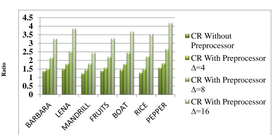
Another set of experimentation is done where pre-processing block is added before context and modeller block to increase the CR. The value of ∆ is varied from 4, 8 to 16. Results of the proposed algorithm are given in Table 2. It is clear from the results that compression ratio increases as the ∆ value increases and corresponding PSNR value decreases. From Table 2, we can observe that as the ∆ value increases from 4, 8, 16, the compression ratio for pepper image also increases from 1.844, 2.679, and 4.208 respectively. Table 2 shows that highest compression ratio of 4.208 is achieved for ∆=16, with the comparable PSNR ratio of 24.697.

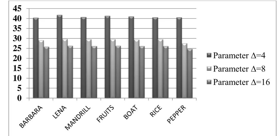
Performance of the algorithm can be observed from the graph in fig.7, which shows variation of CR with different values of ∆ for different test images. It can also be observed that the compression ratio increases as the ∆ parameter increases and the corresponding decrease in PSNR ratio is shown by the fig.8, which degrades the quality of the reconstructed image. Thus the proposed scheme gives better CR than that of other schemes as the ∆ value increases.

TABLE 1. Results of proposed compression algorithm without pre-processing block

Images Huffman CR

Number of Bits Before Compression

Number of Bits After Compression

BARBARA 1.377 405000 294117

LENA 1.502 524288 269640

MANDRILL 1.236 405000 327669

FRUITS 1.400 405000 289285

BOAT 1.454 405000 278541

RICE 1.277 524288 317149

PEPPER 1.581 329672 256166

{

Figure 7: Variation of CR with different values of ∆ for different test images

0

0.5

1

1.5

2

2.5

3

3.5

4

4.5

CR Without

Preprocessor

CR With Preprocessor

∆=4

CR With Preprocessor

∆=8

CR With Preprocessor

∆=16

TABLE 2. Results of proposed compression algorithm with pre-processing block for different value of ∆

Images Pre-processor with Δ=4 Pre-processor with Δ=8 Pre-processor with Δ=16

CR PSNR(dB) CR PSNR(dB) CR PSNR (dB)

BARBARA 1.529 40.466 2.1630 29.090 3.275 25.813

LENA 1.792 41.832 2.5525 29.750 3.874 26.256

MANDRILL 1.465 40.781 1.8179 29.562 2.456 26.191

FRUITS 1.578 41.445 2.2132 29.693 3.298 26.332

BOAT 1.800 41.044 2.4573 29.446 3.700 26.098

RICE 1.497 40.609 2.2357 29.655 3.556 26.172

PEPPER 1.844 40.677 2.6790 27.650 4.208 24.697

(c) PEPPER

(a) LENA (b) BARBARA

Figure 6: Different standard test images

Co

mp

re

ss

io

n

Ra

Figure 8: Variation of PSNR with different values of ∆ for different test images

5.

CONCLUSION

In this paper, we have proposed a low complexity, high and near-lossless image compression algorithm which is a modification to the JPEG-LS algorithm. The average compression ratio achieved is 1.403 for completely lossless compression. The experimental results show that the proposed method gives comparable CR to that of JPEG-LS algorithm and as the ∆ value increases CR increases. Thus for pepper image, CR of 4.208 is achieved. The proposed algorithm has low complexity and high efficiency with the low memory cost suitable for hardware implementation. The algorithm can be applied in satellite imaging, medical imaging etc. Some compression technique achieves good compression ratio but they are complex, in such cases the proposed algorithm can be helpful.

6.

REFERENCES

[1] Sujatha S. Swamy, Mamatha A.S, Vipula Singh, “Satellite Image Compression Techniques”, National Conference on Computational Intelligence & Applications (NCCIA) accepted 6th Feb 2012.

[2] Guoxia Yu, Tanya Vladimirova, MartinN. Sweeting “Image compression systems on board satellites” Surrey Space Centre, University of Surrey, Guildford, Surrey GU27XH, UK Surrey Satellite Technology Limited, Tyco House, Stephenson Road, Surrey Research Park, Guild ford GU27YE, UK accepted 16 December 2008.

[3] M. Klimesh, V. Stanton, and D. Watola, “Hardware implementation of a lossless image compression algorithm using a field programmable gate array,” NASA JPL, California Inst. Technol., Pasadena, 2001.

[4] Guoxia Yu; Vladimirova, T.; Sweeting, M.N.; Surrey Space Centre, Univ. of Surrey, Guildford, UK “FPGA-based onboard multi/hyperspectral image compression system” in Geoscience and Remote Sensing Symposium, IEEE International, IGARSS 12-17 July 2009.

[5] Nunez-Yanez, J.L et al. “Statistical Lossless Compression of Space Imagery and General Data in a Reconfigurable Architecture” in: Adaptive Hardware

and Systems, 2008. AHS '08. NASA/ESA Conference on 22-25 June 2008.

[6] Pizzolante, R.; Dipt. di Inf. ed Applicazioni R. M. Capocelli, Univ. degli Studi di Salerno, Fisciano, Italy “Lossless Compression of Hyperspectral Imagery” in Data Compression, Communications and Processing (CCP), First IEEE International Conference on 21-24 June 2011.

[7] Takada, J.; et al., “A Fast Progressive Lossless Image Compression Method for Space and Satellite Images” in Geo-science and Remote Sensing Symposium, IGARSS IEEE International on 23-28 July 2007.

[8] Ze Wang, et.al. “A High Performance Fully Pipelined Architecture for Lossless Compression of Satellite Image”, in Multimedia Technology (ICMT), International Conference on 29-31 Oct. 2010IEEE.

[9] Cheng-Chen Lin; Yin-Tsung Hwang; Dept. of Electr. Eng., Nat. Chung Hsing Univ., Taichung, Taiwan “An Efficient Lossless Compression Scheme for Hyperspectral Images Using Two-Stage Prediction” in Geoscience and Remote Sensing Letters, IEEE on July 2010 Volume:7, Issue-3.

[10]Xiang Xie, Guolin Li, and Zhihua Wang, “A Low-Complexity and High-Quality Image Compression Method for Digital Cameras” received Aug. 18, 2005; ETRI Journal, Volume 28, Number 2, April 2006.

[11]M. J. Weinberger, G. Seroussi, and G. Sapiro, “LOCO-I: A Low Complexity, Context-Based, Lossless Image Compression Algorithm,” Proc. of the 1996 Data Compression Conference (DCC’96), Snowbird, Utah, pp. 141-149, March 1996.

[12]M. Weinberger and G. Seroussi, “From LOCO-I to the JPEG-LS standard,” HP Laboratories, Palo Alto, CA,

1999. [Online]. Available:

http://www.hpl.hp.com/techreports/1999/HPL-1999-3.pdf

[13]M. Weinberger, G. Sapiro, and G. Seroussi, “The LOCO-I lossless image compression algorithm: Principle and

0

5

10

15

20

25

30

35

40

45

Parameter ∆=4

Parameter ∆=8

Parameter ∆=16

P

standardization into JPEGLS,” IEEE Trans. Image Process., vol. 9, no. 8, pp. 1309-1324, Aug. 2000.

[14]M. Ferretti and M. Boffadossi, “A parallel pipelined implementation of LOCO-I for JPEG-LS,” in Proc. ICPR, 2004, vol. 1, pp. 769–772.

[15]Xiaowen Li, Xinkai Chen, Xiang Xie, Guolin Li, Li Zhang, Chun Zhang, Zhihua Wang, “A Low Power, Fully Pipelined JPEG-LS Encoder for Lossless Image Compression” ICME 2007, pp. 1906 1909,2007.

[16]Markos Papadonikolakis, et.al, “Efficient High-Performance ASIC Implementation of JPEG-LS Encoder”, received on 29 May 2007;

[17]Chien Wen Chen et.al, “A Modified JPEG-LS Image Compression Scheme for Low Bit-Rate Application”, in International Multi Conference of Engineers and Computer Scientists 2008 Vol I IMECS 2008, 19-21 March, 2008, Hong Kong.