Effect of Annealing Selection Operators in Genetic Algorithms on Benchmark Test Functions

Effect of Annealing Selection Operators in Genetic

Algorithms on Benchmark Test Functions

Rakesh Kumar

DCSA, Kurukshetra University, Kurukshetra, Haryana-136119, India

Jyotishree

DCSA, Guru Nanak Girls College, Yamunanagar, Haryana - 135001, India

ABSTRACT

The strategies to find optimal solutions can be broadly categorized into two: exploration and exploitation, but it has been shown in the literature that none can be claimed better than others in all the problems or all stages of the problems. In evolutionary approaches such as genetic algorithm, different operators used are inclined either towards exploration or exploitation but problems demand the operators having the blend of both. In this paper an annealed selection operator has been proposed, the behavior of which is controlled by the current generation i.e. in early cycle of evolution it is more like exploration and gradually it shifts towards exploitation. The experiments have been conducted using five different benchmark functions and implementation is carried out using MATLAB. Results show the improvement over existing selection operators.

Keywords

Benchmark functions; genetic algorithm; rank selection; roulette wheel; selection.

1.

INTRODUCTION

Genetic algorithms are adaptive algorithms proposed by John Holland in 1975 [1] and were described as adaptive heuristic search algorithms [2] based on the evolutionary ideas of natural selection and natural genetics by David Goldberg. They are powerful optimization techniques that employ concepts of evolutionary biology to evolve optimal solutions to a given problem. Genetic algorithm works with a population of individuals represented by chromosomes. Each chromosome is evaluated by its fitness value as computed by the objective function of the problem. The population undergoes transformation using three primary genetic operators – selection, crossover and mutation which form new generation of population. This process continues to achieve the optimal solution. Basic algorithm of genetic algorithm is: Procedure GA(fnx, n, r, m,ngen)

//fnx is fitness function to evaluate individuals in population // n is the population size in each generation (say 10) // r is fraction of population generated by crossover (say 0.7) // m is the mutation rate (say 0.01)

//ngen is total number of generations P := generate n individuals at random // initial generation is generated randomly nogen:=1 //denotes current generation number //define the next generation S of size n while nogen <=ngen do

{ //Selection step: L:= Select(P,n,nogen)

// n/2 individuals of P selected using any selection method

//Crossover step: S:= Crossover(L,n)

// Generates n chromosomes using arithmetic crossover //Mutation step:

Mutation(S,m)

//Inversion of chromosomes with mutation rate m //Replacement step:

P:=S

pb(i):=min(fitfn(P)) // store best individual in population i:=i+1

}

best:=min(pb) //finds best individual in all generations end proc

operators on benchmark test problems. The paper is organized in the following sections. In section 2, related literature review is given on different researches on selection operators and benchmark test problems. Selection methods, their computation formulae and their algorithms are described in section 3. Benchmark test functions considered for implementation are described in section 4. Implementation procedure and computational results are provided in section 5 and concluding remarks are given in section 6.

2.

RELATED WORK

Holland showed that both exploration and exploitation are used optimally by genetic algorithm at the same time using k-armed bandit analogy [1]. This work is also described by David Goldberg [2]. It has been observed that due to certain parameters, stochastic errors occur in genetic algorithms and this may lead to genetic drift [6,7]. In certain cases, selection operation gets biased towards highly fit individuals. This can be avoided by use of Rank Selection technique. Rank scaling ranks the individuals according to their raw objective value [2]. Another problem that arises with genetic algorithms is premature convergence which occurs when the population reaches a state where genetic operators can no longer produce offspring that outperforms their parents [8]. This would likely trap the search process in a region containing a non-global optimum and would further lead to loss of diversity. Al jaddan et al. compared the roulette wheel selection GA (RWS) and ranked based roulette wheel selection GA (RRWS), by applying them on eight test functions from the GA literature [9]. They concluded that RRWS outperformed the conventional RWS in convergence, time, reliability, certainty, and more robustness.

Wang et.al proposed a new hybrid of genetic algorithm and simulated annealing, referred to as GSA and then evaluated its performance against a standard set of benchmark functions [10]. Notably, there was remarkable improvement in performance of Multi-niche crowding PGSA and normal PGSA over conventional parallel genetic algorithm. Liu et.al. proposed a new heuristic algorithm for classical symmetric TSP and tested its performance against benchmark TSP problems [11]. They presented overlapped neighbourhood based local search algorithm to solve TSP and concluded that the proposed algorithm is superior in terms of average deviation and smallest deviation from optimal solutions. In order to improve the balance between the exploration and exploitation in differential evolution algorithm, Sa Angela et al. proposed a modification of the selection that was successful in avoiding entrapment in local optima and could be helpful in many real world optimization problems [12]. R.Thamilselvan and P.Balasubramanie presented a Genetic Tabu search Algorithm (GTA) for TSP and compared with Tabu search [13]. They concluded that GTA is better than GA and TS. Elhaddad and Sallabi proposed a new Hybrid Genetic and Simulated Annealing Algorithm (HGSAA) to solve the TSP [14]. The proposed hybrid algorithm combined both the SA and GAs, in order to help each other overcome their problems to obtain the best results in the shortest time. HGSAA improved the convergence rate of the algorithm with better solutions to TSP compared with other algorithms.

3.

SELECTION

Selection is the first genetic operation in the reproductive phase of genetic algorithm. Its purpose is to choose the fitter individuals in the population that will create offsprings for next generation, commonly known as mating pool. The mating pool thus selected takes part in further genetic

operations, advancing the population to the next generation and hopefully close to the optimal solution. Selection of individuals in the population is fitness dependent and is done using different algorithms [15]. Selection chooses more fit individuals in analogy to Darwin’s theory of evolution – survival of fittest [16]. Too strong selection would lead to sub-optimal highly fit individuals and too weak selection may result in too slow evolution [17]. There are many methods in selecting the best chromosomes. Some are roulette wheel selection, rank selection, steady state selection and many more. The paper focuses on roulette wheel, rank selection and compares their performance with the proposed annealed selection operator.

Some of the symbols used in the algorithms are listed below: ngen → total number of generations

nogen → current number of generation n → total population size

Fj → fitness of jth individual in population rj → rank of jth individual in population mpool → number of chromosomes in mating pool Fbest → Best Fitness value i.e. minimum value of fn(x) Favg → Average Fitness of the population

FXj → fitness of jth individual in Annealed Selection

3.1

Roulette Wheel Selection

Roulette wheel is the simplest selection approach. In this method all the chromosomes (individuals) in the population are placed on the roulette wheel according to their fitness value [2,15,18]. Each individual is assigned a segment of roulette wheel. The size of each segment in the roulette wheel is proportional to the value of the fitness of the individual - the bigger the value is, the larger the segment is. Then, the virtual roulette wheel is spinned. The individual corresponding to the segment on which roulette wheel stops is then selected. The process is repeated until the desired number of individuals is selected. Individuals with higher fitness have more probability of selection. This may lead to biased selection towards high fitness individuals. It can also possibly miss the best individuals of a population. There is no guarantee that good individuals will find their way into next generation. Roulette wheel selection uses exploitation technique in its approach.

Algorithm of Roulette wheel selection is given below. Here, cj is variable storing cumulative fitness and r is random number generated between given interval.

Roulette wheel selection Set l=1, j=1, i=nogen, S=0 While j<=n

{

S=S+Fj //calculates sum of fitness of all individuals }

While l <= mpool {

Generate random number r from interval (0,S) Set j=1

While j <= n {

cj=cj-1+Fj //computes cumulative fitness

If r<=cj, Select the individual j }

3.2

Rank Selection

Rank Selection sorts the population first according to fitness value and ranks them. Then every chromosome is allocated selection probability with respect to its rank [19]. Individuals are selected as per their selection probability. Rank selection is an explorative technique of selection. Rank selection prevents too quick convergence and differs from roulette wheel selection in terms of selection pressure. Rank selection overcomes the scaling problems like stagnation or premature convergence. Ranking controls selective pressure by uniform method of scaling across the population. Rank selection behaves in a more robust manner than other methods [20,21]. In Rank Selection, sum of ranks is computed and then selection probability of each individual is computed as under:

rsumi = ∑Ni=1ri,j (2)

where i varies from 1 to ngen and j varies from 1 to N. PRANKi = ri,j / rsumi (3) Algorithm of Rank selection is given below. Here, ci is variable storing cumulative fitness and r is random number generated between given interval.

Rank Selection

Set l=1, j=1, i=nogen,rsum=0 While j<=n

{ rsum, =rsum+rj } Set j=1

While j<=N { PRANKj=rj/rsum} While l <= mpool {

Generate random number r from interval (0,rsum) Set j=1, S=0

While j<=n {

cj=cj-1+PRANKj //compute cumulative rank

If r<=cj, Select the individual j }

l=l+1 }

3.3

Annealed Selection

The proposed annealed selection approach is to gradually move the selection criteria from exploration to exploitation so as to obtain the perfect blend of the two techniques. In this method, fitness value of each individual is computed. Depending upon the current generation number of genetic algorithm, selection pressure is changed and new fitness contribution, FXj of each individual is computed. Selection probability of each individual is computed on the basis of FXj. As the generation of population changes, fitness contribution changes and selection probability of each individual also changes. The annealed selection operator computes fitness of individual depending on the current number of generation as under:

FXj = Fj / ((ngen+1) – nogen) (4)

Where ngen is total number of generations and nogen refers to current generation number.

Algorithm of Proposed Annealed Selection is given below. Here, ci is variable storing cumulative fitness and r is random

number generated between given interval. Proposed Annealed Selection

Set l=1, j=1, i=nogen While j<=n

{

FXj = Fj / ((ngen+1)-nogen)

//compute fitness for annealed selection }

Set j=1, S=0 While j<=n {S=S+FXj } While l <= mpool {

Generate random number r from interval (0,S) Set j=1, S=0

While j<=n {

cj=cj-1+FXj

If r<=cj, Select the individual j }

l=l+1 }

4.

TEST FUNCTIONS

Many researchers have used different function groups to analyse the performance of genetic algorithms. In this paper, we examine 5 different functions in order to study performance of genetic algorithms and effect of three selection operators. Table 1 lists the five test functions – their names, type and their description.

Table 1: List of Benchmark Test Functions

The first three test functions have been proposed by Dejong. All test functions reflect different degrees of complexity. Test functions F1–F3 are unimodal (i.e.,containing only one optimum), whereas the other test functions are multimodal (i.e. containing many local optima, but only one global optimum).

Sphere [F1] is simple quadratic parabola. It is smooth, unimodal, strongly convex, symmetric [22,23].

𝑓

𝑥 =

𝑥

𝑖=0 -5.12 ≤ xi ≤ 5.12 global minimum: xi=0 fn(x)=0

Function Name Type

F1 Sphere Function Unimodal

Figure 1: Function Graph for F1 for n=2

Rosenbrock [F2] is considered to be difficult, because it has a very narrow ridge. The tip of the ridge is very sharp, and it runs around a parabola. The global optimum is inside a long, narrow parabolic shaped flat valley [22,23].

𝑓2 𝑥 = 𝑛−1𝑖=1 100. 𝑥𝑖+1− 𝑥𝑖2 2+ 1 − 𝑥𝑖 2 -2.048 ≤ xi ≤ 2.048

global minimum: xi=1 fn(x)=0

Figure 2: Function Graph for F2 for n=2

c t

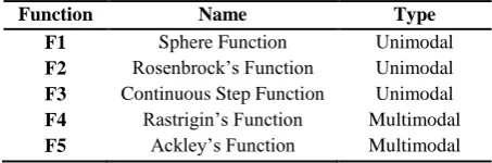
Continuous Step Function [F3] is the representative of the problem of flat surfaces. Function F3 is piecewise continuous step function [22,23].

𝑓3 𝑥 = 𝑛𝑖=1𝑖𝑛𝑡 𝑥𝑖

-5.12 ≤ xi ≤5.12

global minimum: xi=0 fn(x)=0

Figure 3: Function Graph for F3 for n=2

The Rastrigin, Ackley [F4,F5] functions are typical examples of non-linear multimodal functions. Rastrigin’s function [F4] is highly multimodal and has a complexity of O(nln(n)), where n is the number of the function parameters. This function contains millions of local optima in the interval of consideration. It has several local minima [22,23].

𝑓4 𝑥 = (𝑥𝑛𝑖=1 𝑖2− 10. cos 2. 𝜋. 𝑥𝑖 )

-5.12 ≤ xi ≤ 5.12

global minimum: xi=0 fn(x)=0

Figure 4: Function Graph for F4 for n=2

Ackley’s function [F5] is a widely used multimodal test function. The Ackley Function is a continuous, multimodal function obtained by modulating an exponential function with a cosine wave of moderate amplitude. Its topology is characterized by an almost flat outer region and a central hole or peak where the modulations by the cosine wave become more and more influential [22,23].

𝑓5 𝑥 = 𝑎 + 𝑒 − 𝑎. 𝑒

−𝑏. 𝑛𝑖=1_𝑛𝑥𝑖2

− 𝑒 cos 𝑐.𝑥𝑖 𝑛

𝑖=1 𝑛

a=20. b=0.2, -30 ≤ xi ≤ 30

global minimum: xi=0 fn(x)=0

Figure 5: Function Graph for F5 for n=2

5.

IMPLEMENTATION AND

OBSERVATION

In this paper, MATLAB code has been developed to assess the performance of genetic algorithm by using three different selection techniques on the same population for its implementation using the same initial population. Except selection criteria, all other factors affecting the performance of genetic algorithm are kept constant. The code considers a set of 5 benchmark functions. Average and minimum value of fn(x) in each generation is computed over 50 and 100 generations and plotted to compare the performance of three approaches.

The purpose of this implementation is to measure the performance of proposed annealed selection in comparison to roulette wheel and rank selection. This section contains the results obtained from various runs of the code. The comparison of selection techniques is based on their respective performance estimated as the value of the function. The following parameters are used in this implementation:

 Population size (N): 3,5,10 and 20

 Population selection method: Roulette Wheel Selection (RWS), Rank Selection (RS) and Proposed Annealed Selection (AS)

 Crossover Operator: Simple arithmetic crossover

 Mutation: Inversion with mutation probability 5%

 Algorithm ending criteria: Execution stops on reaching ngen generations

 Fitness Function: Objective value of function

Average and Minimum value of evaluation of each function is recorded and examined for further analysis.

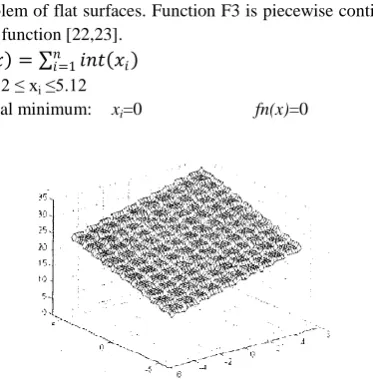
Table 2 : Average and Minimum value of fn(x) in F1

Figure 6: Comparison of Average value of fn(x) in F1 Figure 7: Comparison of Minimum value of fn(x) in F1

N 3 5 10 20

Gen=50 RWS Min 4.93E-37 3.09E-34 4.74E-33 1.46E-31 Avg 0.628 1.179 2.162 5.262 RS Min 5.73E-31 2.85E-30 5.54E-31 2.21E-30

Avg 0.665 1.1346 2.176 5.122 AS Min 8.89E-38 3.32E-35 2.44E-34 1.53E-32

Avg 0.709 1.0545 2.482 5.155 Gen=100 RWS Min 1.93E-72 1.67E-70 4.87E-66 4.32E-65

Avg 0.408 0.46 1.374 2.816 RS Min 1.18E-60 1.11E-64 5.20E-60 1.37E-60

Avg 0.417 0.488 1.353 2.863 AS Min 7.21E-74 8.01E-74 2.24E-69 1.51E-66

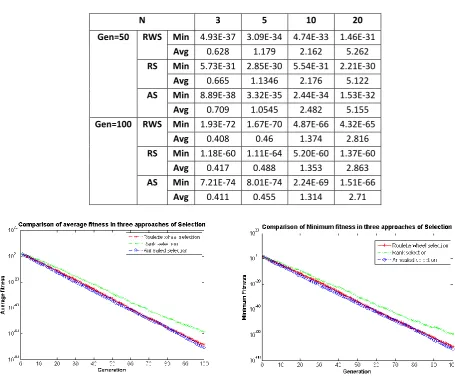
Table 3 : Average and Minimum value of fn(x) in F2

Figure 8: Comparison of Average value of fn(x) in F2 Figure 9: Comparison of Minimum value of fn(x) in F2 Table 4 : Average and Minimum value of fn(x) in F3

N 3 5 10 20

Gen=50 RWS Min 1.8951 3.8781 8.9686 18.9999 Avg 14.3878 34.5157 98.7727 267.7132 RS Min 1.1274 3.9011 8.9738 18.9973

Avg 14.3573 38.7858 110.1202 271.9678 AS Min 1.9642 3.8918 8.8512 18.9502

Avg 14.1299 35.7353 105.7585 257.652 Gen=100 RWS Min 1.818 3.9329 8.9625 18.9913 Avg 14.6431 41.0678 51.9153 118.785 RS Min 1.9893 3.9999 9 18.9962 Avg 14.8046 42.8148 54.4672 119.1835 AS Min 1.9411 3.9258 8.9866 18.9985

Avg 13.7012 39.6808 53.4466 119.699

N

3

5

10

20

Gen=50

RWS Min

1.09E-16 5.33E-17 5.14E-16 3.99E-15

Avg

0.312

0.42393

0.98183

2.0637

RS

Min

6.57E-16 8.59E-16 9.35E-14 2.63E-13

Avg

0.27969

0.49485

1.0676

2.065

AS

Min

1.52E-18 6.72E-18 3.11E-16 1.26E-15

Avg

0.25408

0.40432

0.93658

1.986

Gen=100 RWS Min

5.93E-35 2.02E-34 7.66E-33 1.60E-32

Avg

0.11417

0.21006

0.47329

0.98294

RS

Min

1.14E-30 5.14E-31 4.02E-30 2.16E-31

Avg

0.16419

0.25567

0.47437

0.94699

AS

Min

6.48E-37 3.13E-35 1.95E-33 1.22E-32

Figure 10: Comparison of Average value of fn(x) in F3 Figure 11: Comparison of Minimum value of fn(x) in F3

Table 5 : Average and Minimum value of fn(x) in F4

Figure 12: Comparison of Average value of fn(x) in F4 Figure 13: Comparison of Minimum value of fn(x) in F4

N 3 5 10 20

Gen=50 RWS Min 70 50 8.9813 -100 Avg 73.4838 55.4561 99.8336 -78.1042

RS Min 70 50 9 -100

Avg 73.0887 56.7271 100.3791 -78.4591

AS Min 70 50 8.9622 -100

Avg 73.6985 56.8295 96.1036 -77.8765 Gen=100 RWS Min 70 50 8.9813 -100

Avg 72.0275 53.192 95.036 -87.6698

RS Min 70 50 9 -100

Avg 71.9712 53.0511 96.1081 -88.4613

AS Min 70 50 8.9622 -100

Table 6 : Average and Minimum value of fn(x) in F5

Figure 14: Comparison of Average value of fn(x) in F5 Figure 15: Comparison of Minimum value of fn(x) in F5

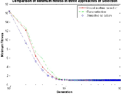
Numerous research efforts have been made to study the performance of different selection operators. In order to study the effect of existing selection operators and proposed annealed selection operator, the implementation has been carried out by keeping the factors initial population, crossover type and its probability, mutation type and mutation rate constant in all the cases. Test runs are carried out for 50 generations as well as 100 generations and four different population sizes. The results for the 5 benchmark functions in terms of average and minimum value are summarized in Table 2,3,4,5 and 6. Figures 6,7,8,9,10,11,12,13,14 and 15 show the performance curves of the three selection operators in terms of average and minimum value of fitness function for population size 20 and 100 generations.

It has been observed that in maximum cases proposed annealed selection has outperformed the roulette wheel selection and rank selection. It can be clearly seen that in early runs of generation, the annealed selection explores the search space and as the number of generations increases, there is increased selection pressure and the annealed selection uses

exploitation mechanism in selecting the individual. In early generations, the behavior of proposed annealed selection is just like the rank selection and gradually it transforms into roulette wheel selection and elitism, this justifies that annealed selection is perfect blend of exploration and exploitation.

6.

CONCLUSION

In maximum optimization problems, it has been observed and stated in the literature that there is no single cure for all the ills. Sometimes exploration techniques outsmart exploitation techniques and vice-versa. Influenced by these observations a number of selection operators have been proposed but they were either inclined towards exploitation or exploration. But generally requirements necessitate that in the beginning of evolution cycle exploration is better and in the last exploitation. The behavior of annealed selection operator can be easily modified as per requirement by changing the pressure. In this paper index variable representing the current

N

3

5

10

20

Gen=50

RWS Min

1.3684 1.0696 8.88E-16 -4.6708

Avg

1.6662 1.4204 0.28187 -2.3732

RS

Min

1.3684 1.0696 8.88E-16 -4.6708

Avg

1.6623 1.4429 0.29853

2.3372

AS

Min

1.3684 1.0696 8.88E-16 -4.6708

Avg

1.6066 1.4558 0.27037 -2.2904

Gen=100 RWS Min

1.3684 1.0696 8.88E-16 -4.6708

Avg

1.4991 1.2506 0.27216

-3.563

RS

Min

1.3684 1.0696 8.88E-16 -4.6708

Avg

1.51

1.2343

0.277

-3.433

AS

Min

1.3684 1.0696 8.88E-16 -4.6708

generation has been used to control the pressure and as it moves from 1 to last generation, the selection pressure increases accordingly and the same is reflected in the behavior of the annealed operator. The experiments have been conducted on five different benchmark functions and optimistic results are produced.

7.

REFERENCES

[1] Holland J. 1975. Adaptation in natural and artificial systems. University of Michigan Press, Ann Arbor. [2] Goldberg D.E. 1989. Genetic algorithms in search,

optimisation, and machine learning. Addison Wesley Longman, Inc. ISBN 0-201-15767-5.

[3] Merz P. and Freisleben B. 1977. Genetic Local Search for the TSP: New results. In Proceedings of IEEE International Conference on Evolutionary Computation, IEEE Press, 159-164.

[4] Ray S., Bandyopadhyay S. and Pal S.K. 2007. Genetic operators for combinatorial optimization in TSP and microarray gene ordering. SpringerScience + Business Media, LLC.

[5] Kumar R. and Jyotishree. 2011. Blending roulette wheel selection & rank selection in genetic algorithms. In Proceedings of 3rd International conference on machine learning and computing, V4, IEEE catalog number CFP1127J-PRT, ISBN 978-1-4244-9252-7, 197-202. [6] Goldberg D.E. and Segrest P. 1987. Finite Markov chain

analysis of genetic algorithms. In Proceedings of the the Second International Conference on Genetic Algorithms. Lawrence Erlbaum Associates, 1-8.

[7] Booker L. 1987. Improving search in genetic algorithms. Genetic Algorithms and Simulated Annealing. Pitman, chapter 5, 61-73.

[8] Fogel D. 1994. An introduction to simulated evolutionary optimization, IEEE Trans. Neural Networks 5 (1), 3-14.

[9] Al jaddan O., Rajamani L. and Rao C.R. 2005. Improved Selection Operator for GA. Journal of Theoretical and Applied Information Technology, 269–277.

[10] Wang Z.G., Rahman M., Wong Y.S. and Neo K.S. 2007. Development of Heterogeneous Parallel Genetic Simulated Annealing Using Multi-Niche Crowding. International Journal of Information and Mathematical Sciences 3:1, 55-62.

[11] Liu S.B., Ng K.M. and Ong H.L. 2007. A New Heuristic Algorithm for the Classical Symmetric Travelling Salesman Problem. International Journal of Computational and Mathematical Sciences. Volume 1, Number 4, 234-238.

[12] Sa Angela A.R., Andrade A.O., Soares A.B. and Nasuto S.J. 2008. Exploration vs. Exploitation in Differential Evolution. Volume 11: In Proceedings of the AISB 2008 Symposium on Swarm Intelligence Algorithms and Applications, ISBN 1 902956 70 2, 57-63.

[13] Thamilselvan R. and Balasubramanie P. 2009. A Genetic Algorithm with a Tabu Search (GTA) for Travelling Salesman Problem. International Journal of Recent Trends in Engineering. Issue I, Vol I, 607 – 610. [14] Elhaddad Y. and Sallabi O. 2010. A New Hybrid Genetic

and Simulated Annealing Algorithm to Solve the Traveling Salesman Problem. In Proceedings of the World Congress on Engineering 2010. Vol. I, ISBN: 978-988-17012-9-9, ISSN: 2078-0958 (Print); ISSN: 2078-0966 (Online), 11-14.

[15] Golberg D.E. and Deb K. 1991. A comparative analysis of selection schemes used in genetic algorithms. Foundations of Genetic Algorithms. San Mateo, CA, Morgan Kaufmann, 69-93.

[16] Fogel D. 1995. Evolutionary Computation, IEEE Press. [17] Mitchell M. 1996. An Introduction to genetic algorithms.

Prentice Hall of India, New Delhi, ISBN-81-203-1358-5. [18] De Jong K.A. 1975. An Analysis of the behavior of a

class of genetic adaptive systems (Doctoral dissertation, University of Michigan). Dissertation Abstracts International 36(10), 5140B University Microfilms No. 76/9381.

[19] Baker J.E. 1985. Adaptive selection methods for genetic algorithms. In Proceedings of an International Conference on Genetic Algorithms and their applications, 101-111.

[20] Whitley D. 1989. The GENITOR algorithm and selection pressure: why rank-based allocation of reproductive trials is best. In Proceedings of the Third International Conference on Genetic Algorithms, Morgan Kaufmann, 116-121.

[21] Back T. and Hoffmeister F. 1991. Extended Selection Mechanisms in Genetic Algorithms. ICGA4, 92-99. [22] Digalakis J.G. and Margaritis K.G. 2002. An

Experimental Study of Benchmarking Functions for Genetic Algorithms. International Journal of Computer Mathematics, 79:4, 403-416.