Quantum Inspired Differential Evolution Algorithm

http://dx.doi.org/10.4236/ojop.2015.42004

Quantum Inspired Differential Evolution

Algorithm

Binxu Li, Panchi Li

School of Computer and Information Technology, Northeast Petroleum University, Daqing, China Email: [email protected]

Received 15 March 2015; accepted 12 May 2015; published 15 May 2015

Copyright © 2015 by authors and Scientific Research Publishing Inc.

This work is licensed under the Creative Commons Attribution International License (CC BY). http://creativecommons.org/licenses/by/4.0/

Abstract

To enhance the optimization performance of differential evolution algorithm, by studying the im-plementation mechanism of differential evolution algorithm, a new idea of incorporating differen-tial strategy and rotation of qubits in the Bloch sphere is proposed in this paper. In the proposed approach, the individuals are encoded by qubits described on Bloch sphere, and the rotation an-gles of qubits in current individual are obtained by differential strategy. The axis of rotation is de-signed by using vector product theory, and the rotation matrixes are constructed by using Pauli matrixes. Taking the corresponding qubits in current best individual as targets, the qubits in cur-rent individual are rotated to the target qubits about the rotation axis on the Bloch sphere. The Hadamard gates are used to mutate individuals. The simulation results of optimizing the mini-mum value of functions indicate that, for an iterative step, the average time of the proposed ap-proach is 13 times as long as that of the classical differential evolution algorithm. When the same limited steps are applied in two approaches, the average optimization result of the proposed ap-proach is 0.3 times as great as that of the classical differential evolution algorithm; when the same running time is applied in two approaches, the average optimization result of the proposed ap-proach is 0.4 times as great as that of the classical differential evolution algorithm. These results suggest that the proposed approach is inefficient in computational ability; however, it is obviously efficient in optimization ability, and the overall optimization performance is better than that of the classical differential evolution algorithm.

Keywords

Quantum Computation, Qubits Encoding, Bloch Spherical Search, Quantum Differential Evolution

1. Introduction

and Price in 1995. This algorithm simulated the “survival of the fittest” natural evolution law. In 2004, Price and others published the first monograph of the algorithm, which has become a classic in the field of DE algorithm

[1]. In 2008, Chakraborty published his work named “Advances in Differential Evolution” [2], in which he made a comprehensive and systematic explanation to the theory, the application and the developing direction in the future of DE. In order to improve the optimization ability of DE algorithm, speed up the convergence and overcome the premature convergence phenomenon of the common heuristic algorithm, many scholars made im-provements on DE algorithm. Ref. [3] proposed a crossover mutation differential evolution algorithm. This me-thod firstly divided the species into two groups according to the fitness, and then selected individuals from two groups respectively and implemented intersection between groups, which could ensure the species had higher diversity. Ref. [4] proposed a self-adaption species adjustment scheme. This method can delete redundant indi-viduals automatically according to the current state of search, which improved the ability of search. Ref. [5]

proposed a method which adjusted the scale factor and the crossover possibility respectively by the Gaussian distribution and the uniform distribution, so that the diversity of the species could be improved. Considering about the impact of population initialization algorithm for optimizing performance, Ref. [6] proposed a new method of the species initialization which was based on quadratic interpolation and nonlinear simplex. In terms of integration with other algorithms, Ref. [7] proposed a self-adaption memetic differential evolution algorithm. Ref. [8] proposed a kind of differential evolution algorithm which was fused with genetic algorithm and applied to the Doppler source of radiation research. The crossover operator used in the classical differential evolution algorithm has a flaw, that is to say, it can only generate one vertex of the super rectangle solid. To address this problem, Ref. [9] proposed a new kind of orthogonal crossover operator. This operator can search more effec-tively in the matrix defined area. Now most majorities of differential evolution algorithms are appropriated for the continuous optimization. For combinatorial optimization, converting real solutions into integer solutions by decoding method is the common way. For this problem, Ref. [10] proposed a differential evolution algorithm based on integer (or discrete) coding. This algorithm effectively improved the optimization efficiency of dealing with the discrete matters by differential evolution algorithm. To enhance the convergence speed of the algorithm, Ref. [11] [12] proposed a new mutation strategy which differed the optimal and the worst individuals at the be-ginning of the algorithm. This method not only effectively balanced the exploration and the development of the algorithm, but also enhanced the ability to detect the solution space. Ref. [13] studied the distributed differential evolution model, and also proposed two new species of migration strategies. These improvements improved the optimization ability of differential evolution algorithm in some extent.

Quantum computing is a new computing model derived from quantum mechanics. At present, in the aspect of integrating particle swarm optimization, the basic theory and the applied research are mature. Sun Jun simulated the particles’ movement to the lowest energy point in the quantum potential well, by which they firstly put for-ward quantum behavior particle swarm algorithm [14]. The core problem of quantum-inspired genetic algorithm is how to design the coding scheme and the evolutionary operators. Currently the most commonly used method of the qubit coding is the one based on the description of the unit circle. The two probability amplitudes of the qubit are both real number, in which there is only one adjustable phase parameter. In regard to the evolutionary operator, the usual way is to change the quantum rotation gate and the quantum NOT-gate with only one phase parameter. However, the real qubit is based on the description of the Bloch sphere, not only the two probability amplitudes of which are complex numbers. It also includes two phase operators. Ref. [15] presented an individ-ual coding method that adopted qubit Bloch coordinate. Even though this method strengthened the characteris-tics of the quantum, it still overlooked the matching relationship between two parameters’ adjustment amount. From the point of the geometry, the bits on the Bloch sphere cannot move to the target bit along the shortest path, so that the optimization ability is limited. Thus, how to design a new kind of coding method and evolutionary operator to enhance the optimization ability of the quantum-inspired evolutionary algorithm is a project deserv-ing further study.

ex-tremum for example, the simulation result shows that the optimization ability of this algorithm is obviously bet-ter than that of the common differential evolution algorithm.

The remainder of the paper is structured as follows. Section 2 gives a brief survey on Common Differential Evolution (CDE) Algorithm. Section 3 describes the basic principle of BQDE algorithm. In Section 4, we test our algorithm using 8 benchmark functions and also compare our results with CDE. Section 5 contains the con-clusions.

2. Differential Evolution Algorithm

Let NP denote the population size, D denote the dimension of the feasible solution space, and X

( )

t denote the population in the tth generation. The initial population is

( )

{

0 0 0

}

1 2 NP

0 = , ,,

X x x x , where 0 0 0 0

,1, ,2, , , i = xi xi  xi D

x .

2.1. Mutation Operation

For any target vector in the parent population xit, differential evolution algorithm can generate the mutation vector vti as follows [16].

(

best

)

(

1 2

)

, 1, 2, , NP

t t t t t t

i = i +λ − i +F r − r i= 

v x x x x x , (1)

where

1

t r

x ,

2

t r

x denote individuals selected randomly in the parent generation. r1≠r2 ≠i, λ, F denote the

scaling factors.

2.2. Crossover Operation

Differential evolution algorithm (DE) generated the new crossover vector ,1, ,2, , ,

t t t t

i = ui ui  ui D

u by

restruc-turing every dimension component of the mutation vector vti and the target vector t i

x . The definite crossover method is as follows:

, rand

,

,

, rand CR, or

, , 1, 2, , NP

, rand CR

t i j t

i j _t

i j

v j j

u i j

x

 ≤ =



=_ =

>

  , (2)

where rand is the random number between (0, 1 ) . jrand∈

{

1, 2,,D

}

. CR is the constant between [0, 1].

2.3. Selecting Operation

Differential evolution algorithm adopted the greedy choice strategy. The new individual uit can only be ac-cepted when it is superior to xit. Otherwise,

t i

x would be kept in the next generation of population. Let

( )

(

)

min f x denote the optimization question. The selecting operation is shown as follows.

( ) ( )

( ) ( )

1 , ;

, .

t t t

i i i

t

i _{t t t}

i i i

f f

f f

+ _{= } <

≥ 

u u x

x

x u x

, (3)

By the selecting operation, differential evolution algorithm makes the individuals in the child population are always better than that in the parent population. This can make the population always evolve in the direction of the optimal solution.

3. The Basic Principle of BQDE Algorithm

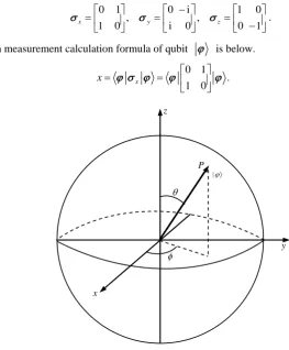
3.1. The Qubit Description Based on Bloch Sphere

In the quantum computation, qubit has two ground states: 0 and 1 . According to the principle of su-perposition, qubit can be expressed by the linear combination of the two ground states.

i cos 0 e sin 1

2 2

ϕ

θ θ

= +

where 0≤ ≤θ π, 0≤ ≤ϕ 2π.

Since θ and φ is continuous, so that one qubit can describe infinite different states. A qubit can be de-scribed by a point on the Bloch sphere. As is shown in Figure 1, where x=cos sinϕ θ, y=sin sinϕ θ,

cos

z= θ. Thus, the qubit ϕ can also be described by the vector in two-dimensional complex Hilbert space as follows.

(

)

T

1 i

,

2 2 1

z x y

z

 _{+ +} 

 

=

 + 

 

ϕ . (5)

Now every point on the Bloch sphere P x y z

(

, ,

)

is corresponds to a qubit ϕ .

3.2. Encoding Method of BQFE

BQDE algorithm encodes individuals by the qubits described based on the Bloch sphere. Let NP denote the population size, D denote the dimension of optimization space, and P

( )

t = p1

( ) ( )

t ,p1 t ,,pNP

( )

t  denote

the t-th generation population. And then the i-th individual pi

( )

0 can be coded (initialized) as follows.

( )

0 1

( )

0 , 2

( )

0 , ,

( )

0

i =  i i  iD 

p ϕ ϕ ϕ , (6)

where

( )

0 cos

(

2 0

)

eiijcos

(

2 1

)

ij ij ij

ϕ

θ θ

= +

ϕ , θ_ij =rand×π, ϕ_ij =rand 2× π.

3.3. Measure of Qubit

According to the principles of Quantum computing, we can acquire the Bloch coordinate

(

x y z, ,

)

of ϕ by the Pauli matrices. This process is called the projection measurement of qubit. The definition of Pauli matrices are shown as follows.

0 1 0 i 1 0

, ,

1 0 i 0 0 1

x y z

−

     

=_{ } =_{ } =_{ }

−

     

σ σ σ . (7)

The projection measurement calculation formula of qubit ϕ is below.

0 1 . 1 0 x

x= = _ _

 

ϕ σ ϕ ϕ ϕ (8)

z

P

θ

φ

|ϕ〉

x

[image:4.595.154.418.390.709.2]

y

0 i

i 0 y

y= = _ −_

 

ϕ σ ϕ ϕ ϕ . (9)

1 0

0 1 z

z= = _ _

−

 

ϕ σ ϕ ϕ ϕ . (10)

3.4. Solution Space Transformation

In BQDE, three optimal solutions made by each individual were expressed by Bloch coordinates. Since the Bloch coordinates

(

x y z, ,

)

∈ −

[

1, 1

]

3, we have to transform the optimal solutions to the actual problem solution space. Set the j-th variable Xj∈ Min ,Maxj j, the solution space transformation can be described as follows.

(

)

(

)

Max 1 Min 1 2

ij j ij j ij

X =_ −x + +x _ , (11)

(

)

(

)

Max 1 Min 1 2

ij j ij j ij

Y =_ −y + +y _ , (12)

(

)

(

)

Max 1 Min 1 2

ij j ij j ij

Z =_ −z + +z _ , (13)

where i=1, 2,, NP, j=1, 2,,D.

3.5. Individual Evolution of BQDE

In BQDE, we will establish the searching mechanism relay on the Bloch sphere, which can make the qubit re-volve around a certain axis towards the target bit. Set t-th generation’s optimal individual as pb

( )

t . For the i-th individual pi

( )

t , we firstly choose two individuals randomly pr₁

( )

t , pr₂

( )

t ,

(

r1 ≠ ≠r2 i

)

, and then let

( )

1 2, ,

r r j t

δ denote the angle between ϕr j₁,

( )

t and ϕr2,j

( )

t , and δi b j, ,

( )

t denote the angle between

( )

, i j t

ϕ and ϕb j,

( )

t . For ϕi j,

( )

t , the rotation angle δi j,

( )

t can be obtained as the follows.

( )

( )

_{1 2}

( )

, , , , , , 1, 2, ,

i j t i b j t F r r j t j D

δ =λδ + δ =  , (14)

where λ,F denote scale factors.

Taking ϕb j,

( )

t on pb

( )

t as target, rotate the ϕi j,

( )

t on pi

( )

t through δi j,

( )

t about axis towards

to ϕb j,

( )

t , and thus the individual’s evolution of pi

( )

t has accomplished.

3.5.1. Determination of the Rotation Axis

In order to rotate ϕi j,

( )

t towards ϕb j,

( )

t , the selection of the rotate axis Raxis

( )

i j, is crucial. Based on

the theory of Hilbert space vector produce, we present the following method.

On the Bloch sphere, set P= p_x,p_y,p_z_ and Q= q q q_x, _y, _z_, which respectively correspond the point P and Q. The axis of rotating the qubits from point P towards to point Q isRaxis = ×P Q.

Set the Bloch coordinates of ϕij

( )

t and ϕbj

( )

t as Pij = pijx,pijy,pijz and Pbj = pbjx,pbjy,pbjz. According to the method above, the axis of rotating ϕij

( )

t towards ϕbj

( )

t is defined as follows.

( )

axis ,

ij bj

ij bj

i j = ×

×

P P R

P P , (15)

where i=1, 2,, NP, j=1, 2,,D.

3.5.2. Determination of the Rotation Matrix

According to the quantum computing principle, the rotation matrix made the qubit revolve about the unit vector axis n= n n n_x, _y, _z_ with a angle δ on the Bloch sphere is below.

( )

cos isin

(

)

2 2

δ δ

δ = − ×

n

R I n σ , (16)

Thus, on the Bloch sphere, the rotation matrix that made the current bit ϕij

( )

t revolve around the axis

( )

axis i j,

R towards to ϕbj

( )

t is given as follows.

( )

( )

( )

( )

(

( )

)

axis cos ₂ isin ₂ axis ,

ij ij ij ij t t i j δ δ

δ = − ×

R

M I R σ , (17)

The rotate operation made the current bit ϕ_ij

( )

t revolve towards to the target bit ϕ_bj

( )

t is below.

( )

_{axis( )},

( )

( )

ij t = i j δij ij t

 MR

ϕ ϕ , (18)

where i=1, 2,, NP, j=1, 2,,D, t denotes the iteration step.

3.5.3. Crossover Operation of BQDE

BQDE adopted the same crossover strategy as CDE does. With help of the recombination of the qubit before and after the individual’s evolution, the new crossover individual qi

( )

t = ϕˆi1

( )

t ,ϕˆi2

( )

t ,,ϕˆiD

( )

t  was generated. Where

( )

( )

( )

, rand CR

ˆ , , 1, 2, , NP

, rand CR

ij ij

ij t

t i j

t  ≤  =_ = >    ϕ ϕ

ϕ , (19)

where rand is the random between

( )

0,1 , CR is the constant between

[ ]

0,1 .

3.5.4. Selected Operation of BQDE

BQDE adopted the same selection strategy with CDE, which is the Greedy Selection Mode. The new individual

( )

i t 

q can be accepted if and only if it’s superior to than pi

( )

t . Otherwise pi

( )

t would be kept into the next generation. Set qi

( )

t and pi

( )

t after the projection measurement and the solution space transformation re-spectively corresponds to

{

X Y Z  , ,

}

and

{

X Y Z, ,

}

, the operation can be described as follows.

(

)

( )

(

( ) ( ) ( )

)

(

( ) ( ) ( )

)

( )

(

( ) ( ) ( )

)

(

( ) ( ) ( )

)

, min , , min , ,

1

, min , , min , ,

i i

i

t f f f f f f

t

t f f f f f f

 _<  + =  ≥        

q X Y Z X Y Z

p

p X Y Z X Y Z

, (20)

where i=1, 2,, NP.

4. Experimental Result Contrasts

4.1. Test Functions

Use the following eight standard test functions to verify the performance of BQDE, and compared with CDE. All eight functions are minimum optimization, which X∗ denotes the minimum extreme value point. All test functions are standard, unconstrained, single objective benchmark functions with different characteristics. For example, the f1

( )

X is multi-modal, non-separable, and has a very narrow valley from local optimum to global

optimum. The f2

( )

X and f3

( )

X are multi-modal, non-separable, asymmetrical, local optima’s number is

huge. The f8

( )

X is multi-modal, non-separable, asymmetrical, continuous but differentiable only on a set of

points.

(1)

( )

1

(

(

2

)

2

(

)

2

)

1 1 100 1 1

D

i i i

i

f X =

∑

₌− x₊ −x + x − , X∈ −

[

30, 30

]

D, f1

( )

X 0

∗ ₌

.

(2) f₂

( )

X 418.982887 1 _iD₁x_isin

( )

x_i

D =

= −

∑

, X∈ −

[

500, 500

]

D, f₂

( )

X∗ =0.

(3) 3

( )

1 2 10 cos 2π

(

)

10

D

i i

i

f X =

∑

₌ _x − x + _, X∈ −

[

5.12, 5.12

]

D, f₃

( )

X∗ =0.

(4)

( )

(

4 2

)

4 1

1

16 5 78.332331 D

i i i

i

f X x x x

D =

=

∑

− + + , X∈ −

[

5, 5

]

D, f4

( )

X 0

∗ ₌

(5)

( )

( )

2 20

5 1sin sin π 29.630884

D _i

i i

ix

f X = − ₌ x _ _+

 

∑

, X∈

[ ]

0,π D, 0f5

( )

X

∗ ₌

.

(6) f6

( )

X =g x x

(

1, 2

)

+ + g x

(

i−1,xi

)

+ + g x

(

D,x1

)

,

( )

(

)

(

(

)

)

0.25 0.1

2 2 2 2 2

, sin 50 1

g x y = x +y _ x +y + _

  ,

2 2

10 , 10 D

X∈ −_ _ , f6

( )

X 0

∗ ₌

.

(7) 7

( )

10 1

(

2 10 cos 2π

(

)

)

D

i i

i

f X = D+

∑

₌ y − y , ,

_{( )}

1 2;

round 2 2 1 2.

i i

i

i i

x x

y

x x

 <



=  _≥

 ,

[

5.12, 5.12

]

D

X∈ − ,

( )

7 0

f X∗ = .

(8)

( )

{

max

(

(

)

)

}

max

(

( )

)

8 1 0 cos 2π 0.5 0 cos π

D k k k k k k

i

i k k

f X =

∑ ∑

_{= = }a b x + _ −D

∑

₌ a b . a=0.5, b=3, kmax =30,

[

0.5, 0.5

]

D

X∈ − , f8

( )

X 0

∗ ₌

.

4.2. Some Definitions

Precision threshold ε: when the preset Maximum Iterative Steps (MIS) reaches, if f X

( )

− f X

( )

∗ <ε, the

algorithm is convergence, otherwise it is not convergence.

Error E: the error definition of a optimized solution X is defined as E= f X

( )

− f X

( )

∗ .

Iterative steps (IS): the iterative steps when the algorithm reaches convergence. If the algorithm is not

con-vergence, set IS = MIS.

Running time (RT): the average time of executing an iteration.

4.3. Parameter Setting

In the CDE algorithms, the range of the scale factor λ= ∈F

[

0.1, 1.0

]

and the crossover probability

[

]

CR∈ 0.1, 1.0 . To determine the most reasonable combination of the three parameters above, we firstly select F, CR from

{

0.1, 0.2,,1.0

}

, which can compose 1000 kinds of combination. Then taking 30-dimension function f1 as example, each combination was optimized 50 times by CDE, and each iteration steps are 1000.

Finally by comparing the average value of the 50 times optimal results, when λ, F is equal to 0.6 and CR is equal to 0.8, the optimization is the best. Thus, in the following experiments, we set λ = =F 0.6 and

CR=0.8 for BQDE and CDE.

Considering the large amount of calculation of the BQDE, we found that the running time of which are about 10 to 20 times to CDE after a lot of simulations. To enhance the credibility of the performance of BQDE, it is necessary to make comparison in the same period of time. Thus, the maximum iteration step is MIS = 104 for BQDE, and is MIS = 104 and MIS = 2 10× 5 for CDE.

The other parameter settings of two algorithms are as follows: Population size NP=100; Function dimen-sion D=30; Precision threshold: for f1, f4, f4,

5

10

ε₌ −

; for f3 and f7, 2

10

ε = ; for f2, ε=1; for

5

f , ε =10; for f6, ε=0.1.

To reflect the superiority of the proposed algorithm and deduce the randomness of it, each function would be optimized 50 times independently by BQDE and CDE. Choose the following items from the 50 optimization results as the comparison index. These items are as follows: the Mean and the standard deviation (STD) of the error E, the Mean and the standard deviation (STD) of the iteration steps, the number of convergence (NC) and the running time (RT).

4.4. Results Comparison and Analysis

The two algorithms were implemented on the computer with 2.0 GHz CPU and 1.0 G RAM, using Matlab7.0 simulation software. The result contrasts of the average error, the standard deviation of error, the number of convergence, and the running time are shown in Table 1. The comparison of the average and the standard devia-tion of the iteradevia-tion steps are shown in Table 2.

[image:8.595.86.538.101.273.2]

Table 1. The mean and standard deviation contrasts of error E for 50 trials.

No.

BQDE CDE

MIS Mean STD NC RT (s) MIS Mean STD NC RT MIS Mean STD NC

f1 104 _{91.4859 138.257 30 0.03972 10}4 _{127.182 300.426 0 0.0019 2 × 10}5 _{94.4472 193.021 0}

f2 104 _{6.76337 145.692 24 0.03594 10}4 _{59.2505 284.889 0 0.0020 2 × 10}5 _{58.6117 272.423 0}

f3 104 _{30.4253 230.262 50 0.03590 10}4 _{110.433 706.128 11 0.0022 2 × 10}5 _{54.3473 290.958 50}

f4 104 0.09968 0.11824 38 0.03688 104 7.04951 6.93309 0 0.0027 2 × 105 6.53958 3.77035 0

f5 104 _{3.67919 1.40779 50 0.03607 10}4 _{13.2842 2.44684 0 0.0030 2 × 10}5 _{10.0863 1.73833 20}

f6 104 _{7.80975 103.729 29 0.03793 10}4 _{22.9041 226.671 0 0.0039 2 × 10}5 _{15.2807 199.598 2}

f7 104 _{24.0999 130.613 50 0.03639 10}4 _{89.6964 239.823 42 0.0027 2 × 10}5 _{44.2251 142.486 50}

[image:8.595.87.538.297.469.2]

f8 104 _{0.18443 0.12594 31 0.44852 10}4 _{0.50029 0.55184 4 0.0345 2 × 10}5 _{0.47342 0.43005 8}

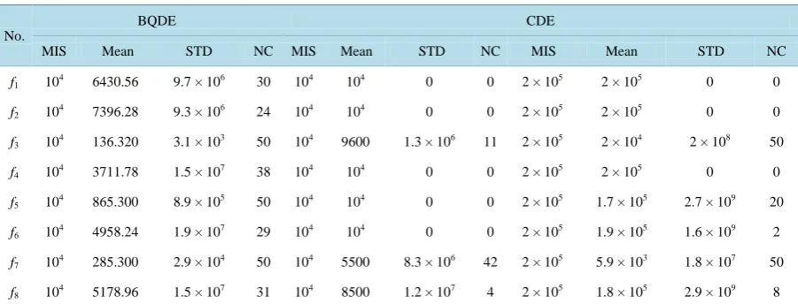
Table 2. The mean and standard deviation contrasts of iterative steps IS for 50 trials.

No.

BQDE CDE

MIS Mean STD NC MIS Mean STD NC MIS Mean STD NC

f1 104 _{6430.56 9.7 × 10}6 _{30 10}4 ₁₀4 _{0 0 2 × 10}5 _{2 × 10}5 _{0 0}

f2 104 _{7396.28 9.3 × 10}6 _{24 10}4 ₁₀4 _{0 0 2 × 10}5 _{2 × 10}5 _{0 0}

f3 104 _{136.320 3.1 × 10}3 _{50 10}4 _{9600 1.3 × 10}6 _{11 2 × 10}5 _{2 × 10}4 _{2 × 10}8 ₅₀

f4 104 _{3711.78 1.5 × 10}7 _{38 10}4 ₁₀4 _{0 0 2 × 10}5 _{2 × 10}5 _{0 0}

f5 104 _{865.300 8.9 × 10}5 _{50 10}4 ₁₀4 _{0 0 2 × 10}5 _{1.7 × 10}5 _{2.7 × 10}9 ₂₀

f6 104 _{4958.24 1.9 × 10}7 _{29 10}4 ₁₀4 _{0 0 2 × 10}5 _{1.9 × 10}5 _{1.6 × 10}9 ₂

f7 104 _{285.300 2.9 × 10}4 _{50 10}4 _{5500 8.3 × 10}6 _{42 2 × 10}5 _{5.9 × 10}3 _{1.8 × 10}7 ₅₀

f8 104 _{5178.96 1.5 × 10}7 _{31 10}4 _{8500 1.2 × 10}7 _{4 2 × 10}5 _{1.8 × 10}5 _{2.9 × 10}9 ₈

only when the iteration steps of two algorithms are the same, but also when the optimization times of two are same. For the experimental results above, we can analysis as follows.

First, BQDE adopted the same DE strategy with CDE so that it obtains the advantages CDE. Second, BQDE coding scheme shows that every individual can give three optimal solutions simultaneously. And the three op-timal solutions would be updated with each iteration step. This effectively enhanced the ergodicity of solution space. Third, BQDE adopted a qubit update method that the qubit rotate on the Bloch sphere about an axis. These methods not only can adjust the two parameters of qubits simultaneously, but also can achieve the best match between the two parameters so that to enhance the efficiency of optimization. Besides, it’s worth pointing out, the computing efficiency of BQDE is pretty low since BQDE involves many matrix operations (such as construct the axis of rotation, revolve operation, projection measurement). As the experiment results show, BQDE’s running time is 10 to 20 times of CDE’s. According to the No Free Lunch Theorem, BQDE gained the performance improvement in expense of scarifying the computing efficiency. BQDE is also obviously better than CDE when comparing with the same period of time (at this time, CDE’s iteration steps is 20 times of BQDE’s). These experimental results show that the CDE’s performance cannot be apparently improved only by extending the iteration step. Therefore the introduction of quantum computing mechanism indeed is an effective way to improve the performance of CDE optimization.

5. Conclusion

method, this method adopted qubit encoding mechanism. For CDE, every dimension variable’s search range of each individual is an internal. While in the proposed algorithm, the variable’s search ranges of every dimension are the Bloch sphere in the three-dimensional space. This algorithm can search the optimized solution on three coordinate axes simultaneously relying on qubit’s pivoting, which can improve the efficiency of optimization. Moreover, the algorithm’s searching range on three coordinate axes is the closed interval

[

−1,1

]

. Then the op-timized solutions for problem can be gained through the solution space transforms. Therefore, this method does not have to consider about the variable’s value range of every dimension during initialization, which is benefit to make uniform optimization strategy. The experimental results showed that it is available to introduce quantum computing mechanism into CDE algorithm to improve the optimization performance. And it also revealed that the combination of realizing individual coding based on quantum bit, computing rotating angle based on CDE strategy, realizing individual updates based on Bloch sphere can enhance the optimization performance of CDE algorithm.

Funding

This work was supported by the National Natural Science Foundation of China (Grant No. 61170132).

References

[1] Price, K., Storn, R. and Lampinen, J. (2004) Differential Evolutionary: A Practical Approach to Global Optimization. Springer, Heidelberg, 183-187.

[2] Uday, K. (2008) Advance in Differential Evolution. Springer, Heidelberg, 287-293.

[3] Zhou, Y.Z., Li, X.Y. and Gao, L. (2013) A Differential Evolution Algorithm with Intersect Mutation Operator. Applied Soft Computing, 13, 390-401. http://dx.doi.org/10.1016/j.asoc.2012.08.014

[4] Zhu, W., Tang, Y., Fang, J.A. and Zhang, W.B. (2013) Adaptive Population Tuning Scheme for Differential Evolution.

Information Sciences, 223, 164-191. http://dx.doi.org/10.1016/j.ins.2012.09.019

[5] Zhang, D.X., Wang, J.H., Gao, L.Q. and Steven, L. (2013) A Modified Differential Evolution Algorithm for Uncon-strained Optimization Problems. Neurocomputing, 120, 469-481.

http://dx.doi.org/10.1016/j.neucom.2013.04.036

[6] Musrrat, A., Millie, P. and Ajith, A. (2013) Unconventional Initialization Methods for Differential Evolution. Applied Mathematics and Computation, 219, 4474-4494. http://dx.doi.org/10.1016/j.amc.2012.10.053

[7] Adam, P.P. (2013) Adaptive Memetic Differential Evolution with Global and Local Neighborhood-Based Mutation Operators. Information Sciences, 241, 164-194. http://dx.doi.org/10.1016/j.ins.2013.03.060

[8] Cao, A.H., Li, W.C. and Li, L.P. (2009) A Passive Location Algorithm Based on Differential Evolution and Genetic Algorithm Using the Doppler Frequency. Signal Processing, 25, 1644-1648.

[9] Wang, Y., Cai, Z.X. and Zhang, Q.F. (2012) Enhancing the Search Ability of Differential Evolution through Orthogonal Crossover. Information Sciences, 185, 153-177. http://dx.doi.org/10.1016/j.ins.2011.09.001

[10] Dilip, D. and Jose, R.F. (2013) A Real-Integer-Discrete-Coded Differential Evolution. Applied Soft Computing, 13, 3384-3393.

[11] Ali, W.M., Hegazy, Z.S. and Motaz, K. (2012) An Alternative Differential Evolution Algorithm for Global Optimization.

Journal of Advanced Research, 3, 149-165. http://dx.doi.org/10.1016/j.jare.2011.06.004

[12] Ali, W.M. and Hegazy, Z.S. (2012) Constrained Optimization Based on Modified Differential Evolution Algorithm.

Information Sciences, 194, 171-208. http://dx.doi.org/10.1016/j.ins.2012.01.008

[13] Cheng, J.X., Zhang, G.X. and Ferrante, N. (2013) Enhancing Distributed Differential Evolution with Multicultural Mi-gration for Global Numerical Optimization. Information Sciences, 247, 72-93.

http://dx.doi.org/10.1016/j.ins.2013.06.011

[14] Fang, W., Sun, J., Xie, Z.P. and Xu, W.B. (2010) Convergence Analysis of Quantum-Behaved Particle Swarm Opti-mization Algorithm and Study on Its Control Parameter. Acta Physica Sinica, 59, 3686-3694.

[15] Li, P.C. and Li, S.Y. (2008) Quantum-Inspired Evolutionary Algorithm for Continuous Spaces Optimization Based on Bloch Coordinates of Qubits. Neurocomputing, 72, 581-591. http://dx.doi.org/10.1016/j.neucom.2007.11.017