How lead exposure relates to temporal changes in IQ, violent crime, and unwed pregnancy

Munich Personal RePEc Archive

How lead exposure relates to temporal

changes in IQ, violent crime, and unwed

pregnancy

Nevin, Rick

15 September 1999

How Lead Exposure Relates to Temporal

Changes in IQ, Violent Crime, and Unwed Pregnancy

Rick Nevin

S

15,

1999

Notice: This is an author’s version of a work that was accepted for publication by Environmental

How Lead Exposure Relates to Temporal

Changes in IQ, Violent Crime, and Unwed Pregnancy

This study compares changes in children’s blood lead levels in the United States with

subsequent changes in IQ, based on norm comparisons for the Cognitive Abilities Test

(CogAT) given to representative national samples of children in 1984 and 1992. The

CogAT norm comparisons indicate shifts in IQ levels consistent with the blood lead to IQ

relationship reported by an earlier study and population shifts in average blood lead for

children under age six between 1976 and 1991. The CogAT norm comparisons also

support studies indicating that the IQ to blood lead slope may increase at lower blood

lead levels. Furthermore, long term trends in population exposure to gasoline lead were

found to be remarkably consistent with subsequent changes in violent crime and unwed

pregnancy. Long term trends in paint and gasoline lead exposure are also strongly

associated with subsequent trends in murder rates going back to 1900. The findings on

violent crime and unwed pregnancy are consistent with published data describing the

relationship between IQ and social behavior. The findings with respect to violent crime

are also consistent with studies indicating that children with higher bone lead tend to

display more aggressive and delinquent behavior. This analysis demonstrates that

widespread exposure to lead is likely to have profound implications for a wide array of

socially undesirable outcomes.

Key Words:

INTRODUCTION

Many studies provide evidence of an inverse relationship between lead exposure and cognitive

abilities (National Research Council). There is, however, disagreement about the IQ to blood lead

slope (IQ points lost per one ug/dl increase in blood lead) and the influence of confounding

variables (Schwartz; Pocock et al.). There is strong evidence that young children face the

greatest risk of IQ losses due to lead exposure, especially during the first three years of life when

basic cognitive abilities develop (Schwartz). Cognitive losses due to lead exposure during the

first three years of life appear to be most evident in IQ tests taken some years later, around age

10 or older, when IQ scores are more stable and predictive of future outcomes (National

Research Council; Schwartz). There is no consensus, however, on whether lead exposure is

more strongly associated with verbal IQ, mathematical skills, or performance IQ (National

Research Council).

In addition to disagreements about the statistical significance of IQ losses due to lead exposure

after controlling for confounding variables, there is a separate debate about the public policy

significance of studies showing only a fraction of an IQ point lost per one ug/dl increase in blood

lead. One argument in favor of public policy initiatives to reduce lead exposure is that small

differences in mean IQ due to lead exposure can result in substantial differences in extreme

values of the IQ and blood lead distributions. Differences in IQ have also been associated with

differences in educational attainment and average lifetime earnings (National Research Council).

A better understanding of the specific nervous system impacts of lead may be obtained from new

epidemiological or laboratory studies, but the public policy debate has been largely resolved, with

policy initiatives already successfully implemented to reduce lead exposure. The second and

third National Health and Nutrition Examination Surveys (NHANES II and III) show that blood lead

in lead in gasoline and solder in food and soft drink cans (Pirkle, et al.). This dramatic decline in

national blood lead levels offers a new research perspective on both the statistical significance of lead’s association with IQ after adjusting for covariates, and the public policy significance of IQ

changes due to lead exposure. Has the decline in childhood blood lead since 1976 resulted in

any subsequent increase in IQ levels that cannot be explained by confounding variables? If IQ

levels have increased, what slope estimate for the IQ to blood lead relationship is suggested by

this increase in IQ? Finally, have changes in blood lead been followed by subsequent changes in

social behavior – with public policy significance – that might be associated with extreme values of

the IQ and blood lead distributions?

Confounding Variables and the IQ to Blood Lead Slope

Most studies attempt to control for established effects on IQ scores such as socioeconomic status

(SES), parental education and parental IQ. Many studies also incorporate the Home Observation for the Measurement of the Environment (HOME) inventory, which measures a child’s family

environment with respect to intellectual stimulation and parental sensitivity, based on a structured

interview and home observation.

“Several of these studies have reported that significant associations between body lead and

children’s developmental test scores disappear or become marginal when HOME is used as

a covariate. [However,] many HOME items can directly reflect the presence of lead and its effect, rather than measuring independent sources of variation in children’s development.

For example, one of the HOME subscales measures quality of the physical environment,

including cleanliness. This measure can be related to lead exposure because of lead in household dust” (Banks et al.).

Schwartz's meta-analysis (1994) of the IQ to blood lead relationship examined eight studies that

controlled for both parental IQ and HOME score, and the eight studies together provided a range

of low, average, and high SES. Schwartz reported an overall slope of .26 IQ points lost per one

ug/dl increase in blood lead, but he found a slope of .323 in studies with mean blood lead below

15 ug/dL, and .232 in studies with mean blood lead above 15 ug/dL. The only study in the

Schwartz analysis with mean blood lead below 10 ug/dL reported a slope of .58 IQ points lost per

one ug/dL increase in blood lead. This last study suggests that an even higher slope might apply

to blood lead levels below 10 ug/dl.

A more recent study by Dudek and Merecz (1997) reports a slope of .53 in a population of 380 children with average blood lead of 10.2 ug/dL, after controlling for covariates including mother’s

education, occupational status, and family income. In this study, blood lead was more strongly associated with verbal IQ than with performance IQ. Although mother’s education exerted the

greatest influence on a child’s IQ, the authors found that higher blood lead was associated with

lower IQ for both higher and lower maternal education groups. The authors also found the most

rapid deterioration of IQ was observed at blood lead levels between 5 - 10 ug/dl and 11 - 15 ug/dl,

consistent with the Schwartz finding of an increasing slope at lower blood lead levels.

Another meta-analysis, by Pocock et al., found that five prospective studies supported an IQ to

blood lead slope estimate of .185, and 14 cross-sectional blood lead studies supported a slope

estimate of .175 after the removal of one extreme value. A negative association was also found in

seven cross-sectional tooth lead studies. All five of the prospective studies controlled for mother’s

IQ and HOME score, and most of the cross-sectional studies controlled for either mother’s IQ or

mother’s education. Pocock and colleagues observed “no striking relation between the studies’

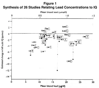
mean blood lead and the magnitude of the lead-IQ association” (Pocock et al.), but the data in this

tooth lead report an average loss of one to two IQ points per doubling of body lead burden (10 to

20 ug/dL blood lead or 5 to 10 ug/g tooth lead), but the four studies of children with average blood

lead levels below 10 ug/dL show an average loss of about four IQ points per doubling of body

lead burden.

Figure 1

Synthesis of 26 Studies Relating Lead Concentrations to IQ

“For each study the estimated change in IQ for a specific doubling of body lead burden (10 to 20 ug/dl blood lead or 5 to 10 ug/g tooth lead) is plotted against the study’s mean blood lead concentration. Study types: P=prospective, C=cross sectional blood lead, T=cross sectional tooth lead. Three sizes of letter represent the size of the study (>400, 200-400, or <200 children). Substantial or partial adjustment for confounders is indicated by a square or circle respectively; the influence of substantial adjustments is shown by the arrowed lines.” (Pocock et al).

Pocock and colleagues also caution that it is difficult to draw clear conclusions about a causal

relationship between lead exposure and IQ, in part because of confounding variables. One

commentary on this analysis, however, suggests that

“the authors ignore the phenomenon of shared variance and assign the decrease in effect

size when confounders are controlled exclusively to the confounder. Confounders can have

a direct affect on outcome; they can also operate through increasing lead concentration.

and surfaces that have deteriorated. Lower parental intelligence and poor care taking, in

addition to directly affecting the cognition of offspring, may lead to increased absorption of lead” (Needleman).

Temporal Trends in IQ

IQ scores measure the cognitive ability of any individual relative to the rest of the population.

Therefore, a temporal shift in the IQ distribution is apparent only when a new population norm, or

standard, is established for a new or revised IQ test based on the distribution of test scores from

a new representative sample of the population. If most people have IQ scores relative to this

new standard that are lower than their IQ scores on an older IQ test (relative to an older

population sample) then this suggests an upward shift in the IQ distribution for the population. In

other words, an increase in cognitive ability for the population as a whole establishes a higher

standard for measuring the IQ of any individual, so that a typical individual will have a lower IQ

score relative to this new, higher standard.

By comparing old and new population standards for IQ tests over time, James Flynn has

documented extensive evidence of rising IQ scores in twenty nations (Flynn, 1994). The IQ

gains reported by Flynn are largest on culture-reduced tests, like the Ravens test; less on tests

that combine performance and verbal scales, like the Wechsler and Stanford-Binet tests; and

lowest on verbal-math tests, like the Otis test (Flynn, 1987).

Culture-reduced tests measure fluid intelligence, or on-the-spot problem-solving ability, as

opposed to learned or acquired knowledge.

“Tests of spatial visualization, figural similarities and sequences, figure classification and

Tests that also measure crystallized intelligence

“place less emphasis on on-the-spot problem solving and more on whether someone has

acquired the skills, or general knowledge, or vocabulary we would expect an intelligent

person to gain in a normal life. IQ gains over time diminish as tests get farther and farther

from measuring fluid intelligence. The continuum from fluid to crystallized runs from tests

with culture-reduced content, through performance tests, through verbal tests, to pure

vocabulary tests. Verbal tests always involve spoken or written language. Performance

tests involve an operation, using blocks to copy a design, arranging pictures in a logical sequence” (Flynn, 1994).

In the United States, Flynn reports an average increase of 0.3 IQ points per year from 1932 to

1989, at a roughly uniform rate and at similar rates for all ages, on the Wechsler and

Stanford-Binet tests that measure a mix of fluid and crystallized intelligence. Furthermore, comparing

Stanford-Binet scores by soldiers in 1918 with the standardization sample in 1932 indicates that

this steady rise in IQ in the United States began no later than 1918 (Flynn, 1994).

In Japan, Austria, West Germany, and France, Wechsler scores for children ages 6 to 15 show

gains of .38 to .84 IQ points per year from the early 1950s through the early 1980s. Children

ages 8 to 12 in Switzerland show a Wechsler gain of .65 IQ points per year from 1956 to 1977,

but only .19 points per year from 1977 to 1984 (Flynn, 1987).

In France, Belgium, and The Netherlands, the culture-reduced portion of military examination

tests, given to young men around the age of 18, show gains of .67 to 1.0 IQ points per year from

the early 1950s through the early 1980s. Similar military tests in Norway show gains of .63 IQ

points per year from 1954 to 1968, but only .22 IQ points per year from 1968 to 1980 (Flynn,

Verbal-math scores on the Belgium and France military tests show gains of .41 and .37 IQ points

per year, respectively. The verbal-math scores on the Norway military tests show gains of .58 IQ

points per year from 1954 to 1968, but show losses of .13 IQ points per year from 1968 to 1980.

Children ages 10 to 13 in New Zealand show verbal test gains of .24 IQ points per year from

1936 to 1968. In Canada, 10-year-old children show verbal test gains of .63 from 1958 to 1978,

but 13-year-old children show lesser gains of .35 IQ points per year over the same time period

(Flynn, 1987).

Flynn examines several possible explanations for rising IQ scores over time, including advances

in education and improved nutrition. He finds that different theories may explain IQ gains in

certain countries over specific time intervals, but no single theory adequately explains all of the

data on IQ gains.

“Some day sufficient data may allow us to see why some tests show higher gains than

others, why some countries show higher gains than others [resulting in] a better theory of intelligence and better vehicles for measuring it.” (Flynn, 1987).

Temporal Trends in Lead Exposure

Changes in lead exposure should be considered as another variable that could be associated

with rising IQ scores over time. Gasoline lead exposure cannot explain the long-term IQ trend

because it did not begin until the 1920s and did not peak until the early 1970s. Exposure to both

paint lead and one major source of lead in drinking water, however, has declined throughout

most of this century in a manner that could have contributed to the long-term rise in IQ levels. “The period during which leaded paint had the highest amounts of lead and posed the

problem with lead connectors and service pipe is associated principally with old housing, built around 1920 or before.” (National Research Council).

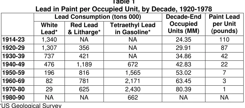
Prior to 1906 practically all house paints contained white lead (Mattiello). Table 1 shows data on

white lead consumption, by decade, from 1914-78 (US Geological Survey). White lead data for

1914-23 in Table 1 are used to estimate 1920s consumption because 1914 is the earliest year of

available data. A small percentage of white lead was consumed in ceramics, chemicals,

greases, plasterizers and stabilizers but the majority of white lead was used in paint (Gipe). In

fact, the paint industry accounted for about 95 percent of total white lead pigment consumption

during the 1930s (Mattiello). Table 1 also shows consumption of tetraethyl lead in gasoline from

1941-87 and consumption of red lead and litharge from 1920-78 (US Geological Survey).

Litharge is primarily used in storage batteries. Red lead was used mostly for ceramics,

lubricants, petroleum, rubber, glass, and other industrial applications, and was used very little in

the paint industry as varnishes, enamels and glazes (Gipe).

The limited application of red lead by the paint industry was often as a rust-inhibiting primer coat

for exterior metals, including bridges and automobiles, which were covered by a finish coat of

different composition (Mattiello). The industrial uses of red lead are especially apparent in the

data for the 1940s when there was a sharp increase in red lead and litharge consumption during

World War II, while housing starts were sharply lower during the same period. The increase in

red lead consumption in 1941 was specifically associated with efforts by the automobile industry

to produce a record number of vehicles before converting to war production (US Geological

Survey). Industrial lead consumption can result in paraoccupational lead exposure for young

children (lead brought home from work exposure, usually on work clothes) but white lead used in

house paint would have the far more pervasive effect on children’s blood lead levels. Therefore,

each decade to estimate the change in paint lead exposure per housing unit from 1914 through

1978. By this measure, it is apparent that average childhood exposure to lead in paint began to

decline at least as far back as the 1920s.

Table 1

Lead in Paint per Occupied Unit, by Decade, 1920-1978

Lead Consumption (tons 000) Decade-End

Occupied Units (MM)

Paint Lead per Unit (pounds) White

Lead*

Red Lead & Litharge*

Tetraethyl Lead in Gasoline*

1914-23 1,340 NA NA 24.35 110

1920-29 1,307 356 NA 29.91 87

1930-39 737 421 NA 34.86 42

1940-49 476 1,189 672 42.83 22

1950-59 196 816 1,565 53.02 7

1960-69 82 781 2,171 63.45 3

1970-80 29 625 2,430 80.39 1

1980-90 NA NA 662 NA NA

*US Geological Survey

Although paint lead in older housing units poses a lingering hazard today, the health hazards

must have been more acute and more widespread in the years when peeling lead paint was

scraped away and replaced with a fresh coat of lead paint. As early as 1839, research revealed “the clinical course of 1,207 persons with lead colic and the types of work that exposed

them to lead. More than 800 of the cases were in painters or workers involved in the manufacture of white or red lead pigments. … Somewhat later … reproductive failures and

congenital lead poisoning … not only among female lead workers, but also among the

wives of men who worked in the lead trades … led a British Royal Commission in 1910 to

recommend that women be excluded from the lead trades” (National Research Council).

In 1987, an advertisement in England for lead-free enamel emphasized that the product was

non-poisonous, in contrast to lead paint. In 1904, research explicitly linked childhood lead

poisoning in Australia to children biting their nails and sucking their fingers after exposure to lead

paint on walls and railings. The first American case of childhood lead poisoning was reported in

1914, and 17 more cases were published in 1926 (National Research Council). During this

“Paint production data from the Census of Manufacturers indicate that, by 1919, the

production of water and calcimin-based paints almost equaled those with white lead.

Around 1920, a zinc-based compound known as lithopone came into use as a supplement

or replacement for white-lead pigments in interior paints. In the 1930s, titanium dioxide

was introduced as a hiding pigment. The production of titanium dioxide pigments equaled

that of leaded pigments by the late 1940s and, by the late 1950s, was five times greater.

Latex paint came into use in the 1930s and, by the 1950s, was the dominant paint for

interior walls. Lead was seldom used with latex paint; it was primarily an additive to oil and alkyd paints” (US Department of Housing and Urban Development, 1970).

Declining childhood exposure to paint lead (and to drinking water lead from lead pipes) could have substantially reduced children’s blood lead levels in the United States from the early 1900s

through the late 1940s. The declining use of lead in paint throughout this century means that the

children living in newer residential units each year were exposed to lead paint on fewer

household surfaces and/or to lower concentrations of lead in the lead-based paint that was in

their home. Children living in older homes that were well maintained also would have less

exposure over time as repainting covered high lead concentration paint with paint that had lower

concentrations of lead or no lead at all.

Comparing Temporal Trends in Lead Exposure and IQ

The likely decline in blood lead over the first half of the 20th century could be a factor in rising IQ scores among adolescents and young adults from 1918 through 1970, covering most of the data

reported by Flynn. The Stanford-Binet scores for US soldiers in 1918 could be associated with

childhood paint lead exposure around 1900 when practically all house-paints contained white

lead. The standardization sample in 1932 could be associated with lead exposure around 1912

and IQ norm comparisons through the early 1970s could reflect the decline in white lead

consumption after the 1920s. Evidence of a similar awareness of lead paint hazards over a

similar time period in other countries suggests that reduced lead exposure could also be a factor

in rising IQ scores in other countries.

US consumption of tetraethyl lead in gasoline first exceeded the consumption of white lead in the

late 1940s, but the expanding use of automobiles probably had very different effects on blood

lead levels for different segments of the population from the 1940s through the 1960s. Children

in central cities had the greatest exposure to gasoline lead, due to urban traffic congestion, and

they realized relatively little benefit from declining levels of lead in paint because older housing

units common in central cities had high concentrations of lead in paint from earlier decades. This

is particularly true because poorer children have been disproportionately concentrated in central

cities, and lower income households are more likely to have paint in poor condition, creating

paint chip and lead dust hazards. During the years when gasoline lead was used extensively,

children exposed to urban atmospheres and to interior lead paint in their homes had about six

times higher daily lead intake than suburban children with minimal lead exposure (US

Environmental Protection Agency). Therefore, the blood lead levels of children in urban areas

exposed to gasoline lead and to paint lead in older housing probably began to rise as early as

the 1940s.

Blood lead levels for most American children, however, may have continued to decline from 1940

through the early 1960s because lower paint lead levels in new suburbs may have more than

offset suburban exposure to gasoline lead. The near doubling of occupied units from 1940 to

1970 (as shown in Table 1) reflects the rapid rate of suburban residential construction in the

1950s and 1960s, and families with young children accounted for a disproportionate share of

certainly had less paraoccupational lead exposure because the industrial consumption of red

lead and litharge also declined over these two decades. Suburban children would also have

experienced the greater decline in paraoccupational exposure to the extent that suburban

parents were more likely to have jobs with little or no risk of occupational lead exposure. A

continuing decline in blood lead levels for suburban children throughout the 1950s and into the

1960s could be a factor in rising average IQ scores among young adults through the 1980s.

By the mid-1960s, US consumption of lead in gasoline far exceeded the consumption of lead in

paint, with tetraethyl lead consumption exceeding 200,000 tons per year from 1964 through

1974.

“Ambient airborne lead concentration showed no marked trend from 1965 to 1977.

Decreases from 1977 to 1982 reflect the smaller lead emissions from mobile sources” (US

Environmental Protection Agency).

Extensive research demonstrates a strong correlation between blood lead levels and lead

consumed in gasoline during the late 1970s, reflecting the combined effects of inhaled air and

gasoline lead deposited on food and in household and street dust (Schwartz and Pitcher; US

Environmental Protection Agency).

The pervasive effects of US gasoline lead exposure from the mid-1960s through the 1970s

suggest that blood lead levels almost certainly rose for most American children during this time

period. Therefore, if childhood lead exposure were a significant factor in the long-term rise in IQ

scores reported by Flynn, then we would expect to see that rising trend interrupted for Americans

born during the 1960s and 1970s. On the other hand, the decline in gasoline lead use and the

exposure were a significant factor in rising IQ scores reported by Flynn, then we would expect to

see that rising trend accelerate for Americans born after 1982.

A similar pattern of declining paint lead exposure over several decades, followed by a sharp

increase in gasoline lead exposure in the 1970s, could explain some of the temporal variation in

long-term IQ trends reported for other nations. For example, Swiss children ages 8 to 12 had

Wechsler gains of .65 IQ points per year from 1956 to 1977 but only .19 IQ points per year from

1977 to 1984. The first of these two norm comparisons (1977 relative to 1956) compared a

population standard for children born around 1967 with a population standard for children born

around 1946. The children born in 1967 had far less childhood paint lead exposure than those

born in 1946, and this decrease in paint lead exposure may have only been slightly offset by an

increase in gasoline lead exposure. The second Swiss comparison (1984 relative to 1977)

compared an IQ norm for children born around 1974 with an IQ norm for children born around

1967. The children born in 1974 would have had only slightly less childhood paint lead exposure

than those born in 1967, and this decrease in paint lead exposure may have been more than

offset by a sharp increase in gasoline lead exposure.

The same pattern appears in Norway military tests for recruits around the age of 18.

Culture-reduced and verbal-math tests in Norway showed gains of .63 and .58 IQ points per year,

respectively, from 1954 to 1968. These increases were followed by culture-reduced gains of .22

IQ points per year and verbal-math losses of .13 IQ points per year from 1968 to 1980. The

1968 norm comparison (relative to 1954) compared young men born around 1950, when paint

and gasoline lead exposure were low, with young men born around 1932, when paint lead

exposure was very high. The 1980 norm comparison (relative to 1968) compared young men

born around 1962, when gasoline lead exposure was higher, with young men born around 1950,

Social Behavior Associated with IQ

Although data on yearly changes in IQ are unavailable, temporal data are available for specific

types of social behavior associated with lower IQ scores. Herrnstein and Murray, in their

controversial book The Bell Curve, cite data showing that individuals with lower IQ levels account

for a disproportionate share of violent crime and unwed births. Needleman and colleagues (1996)

have also shown that higher bone lead levels are associated with an increase in aggressive and

delinquent behavior among boys ages 7 to 10 with similar IQ levels.

Herrnstein and Murray associate IQ with social behavior based on data from the National

Longitudinal Survey of Labor Market Experience of Youth (NLSY), a representative national

sample of American youths. When the NLSY began in 1979, the 12,686 participants were ages

14 to 22. In 1980, 94 percent of these youths were given the Armed Forces Qualification Test

(AFQT). Herrnstein and Murray restated the raw scores on the AFQT in the IQ metric (a mean of

100 and a standard deviation of 15) and refer to these results as IQ scores. To justify the use of

the AFQT as a measure of IQ, the authors show that this test has a very high correlation with

other IQ tests available for some NLSY participants (Herrnstein and Murray).

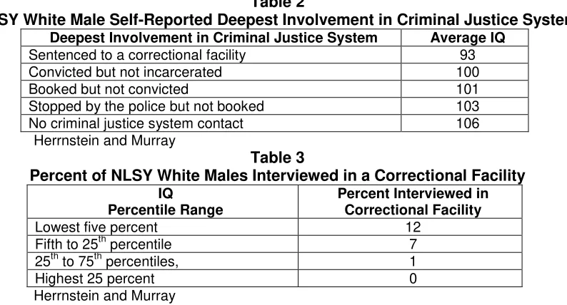
Table 2 shows the average IQ (AFQT) levels of white males in the NLSY by their self-reported

deepest involvement with the criminal justice system (Herrnstein and Murray). As an observed

measure of criminal involvement, the NLSY data also reveal the percentage of white males who

ever had an NLSY interview conducted in a correctional facility, by IQ percentiles, as shown in

Table 3 (Herrnstein and Murray). In addition to the NLSY data, the authors cite research from

Britain, Sweden, Denmark, and New Zealand, and conclude that the research as a whole

indicates that incarcerated offenders have an average IQ of about 92, eight points below the

Table 2

NLSY White Male Self-Reported Deepest Involvement in Criminal Justice System

Deepest Involvement in Criminal Justice System Average IQ

Sentenced to a correctional facility 93

Convicted but not incarcerated 100

Booked but not convicted 101

Stopped by the police but not booked 103

No criminal justice system contact 106

Herrnstein and Murray

Table 3

Percent of NLSY White Males Interviewed in a Correctional Facility

IQ

Percentile Range

Percent Interviewed in Correctional Facility

Lowest five percent 12

Fifth to 25th percentile 7

25th to 75th percentiles, 1

Highest 25 percent 0

Herrnstein and Murray

By focusing exclusively on white males, the data in Tables 2 and 3 remove any confounding due

to racial or gender bias relating to IQ tests and/or to law enforcement. Herrnstein and Murray

also found that both self-reported and observed measures of criminality among white males were

more strongly associated with IQ than with family socioeconomic status.

“In the case of the self-report data, higher socioeconomic status was associated with higher

reported crime after controlling for IQ. In the case of incarceration, the role of

socioeconomic background was close to nil after controlling for IQ, and statistically

insignificant. By either measure of crime, a low IQ was a significant risk factor” (Herrnstein

and Murray).

Herrnstein and Murray also examined confounding due to family demographics, by comparing white males from intact families “consisting of the biological mother and father” with white males

from a “broken” home.

“Although family setting had an impact on crime, it did not explain away the predictive

power of IQ. For example, a young man from a broken family and an average IQ and

socioeconomic background had a 4 percent chance of having been interviewed in jail.

background to the 2d centile instead, and the odds rise only from 4 to 5 percent.) The

same conclusions apply to the measure of self-reported crime” (Herrnstein and Murray).

As shown in Table 4, Herrnstein and Murray also report a strong association between IQ and the

incidence of unwed births among young white women in the NLSY.

Table 4

Unwed Births Among White Females in the NLSY

IQ Percentile Range

Percent of White Females That Have Unwed Births

Percent of White Female First Births That Are Unwed Births

Lowest five percent 32 42

Fifth to 25th percentile 17 23

25th to 75th percentiles 8 13

75th to 95th percentiles 4 7

Highest five percent 2 7

Herrnstein and Murray

Herrnstein and Murray found that socioeconomic status affects unwed birth rates, but did not

explain the predictive power of IQ.

“Higher social status reduces the chances of an illegitimate first baby from about 19 percent

for a woman who came from a very low status family to about 8 percent for a woman from a

very high status family, given that the woman has average intelligence. Let us compare

that 11 percentage point swing with the effect of an equivalent shift in intelligence (given

average socioeconomic background). The odds of having an illegitimate first child drop

from 34 percent for a [woman in the lowest 5 percent of IQ] to about 4 percent for a [woman

in the highest 5 percent of IQ], a swing of 30 percentage points independent of any effect of socioeconomic status” (Herrnstein and Murray).

The role of family demographics was also found to have less influence than IQ on unwed births: “Let us consider a white woman of average intelligence and average socioeconomic

background. The odds that her first child would be born out of wedlock were:

10 percent if she was living with both biological parents.

25 percent if she was living with her mother (with or without a live-in boyfriend).

Consider the case of a young woman at risk, having lived with an unmarried biological

mother at age 14. Given average socioeconomic background and an average IQ, the

probability that her first baby would be born out of wedlock was 25 percent. If she had an

IQ at the 98th centile (an IQ of 130 or above), the probability plunged to 8 percent. If she had an IQ at the 2d centile (an IQ of 70 or below), the probability soared to 55 percent.

High socioeconomic status offered weak protection against illegitimacy once IQ had been taken into account.”

Herrnstein and Murray caution that:

“Despite the relationship of low IQ to criminality, the great majority of people with low

cognitive ability are law abiding.”

They also state that

“the increase in crime over the past thirty years (like the increases in illegitimacy and

welfare) cannot be attributed to changes in intelligence but rather must be blamed on other factors, which may have put people of low cognitive ability at greater risk than before.”

It is certainly true that most people with low cognitive ability are law abiding, and most women

with low cognitive ability do not become pregnant outside of marriage, but this does not mean

that temporal changes in crime and unwed pregnancies are necessarily unrelated to changes in cognitive abilities. The NLSY data suggest that cognitive ability may affect an individual’s

foresight and comprehension of the long-term consequences of crime and unwed pregnancy.

The important role of many other factors means that IQ is a dubious marker for any individual’s

propensity to commit violent crimes or become pregnant outside of marriage, but IQ may affect

illustrated in Table 5 by estimating the potential effect on violent crime per 100,000 population if

the lowest three deciles of the IQ distribution each increased by six points.

Table 5

Illustration of Potential Effect on Crime Rates

Due to a Six Point Upward Shift in IQ for Lowest 30 Percent of the IQ Distribution

IQ Decile Population Violent

Crimes

Median IQ

New IQ New Violent

Crimes

First 10,000 950 74 80 700

Second 10,000 700 84 90 400

Third 10,000 400 90 96 100

4th– 8th 50,000 500 102 102 500

9th and 10th 20,000 0 122 122 0

Violent Crime per 100,000 Population 2,550 1,700

The second column of Table 5 shows the population distribution by IQ decile, assuming a total

population of 100,000. The third column shows the number of violent crimes by IQ decile if we

assume (for the purpose of this illustration) that the percent of NLSY white males interviewed in

jail is representative of the violent crime rate associated with different segments of the IQ

distribution. For example, Table 3 showed that 12 percent of NLSY white males in the lowest

five percent of IQ were interviewed in jail, and 7 percent of those in the 5th to 25th percentiles were interviewed in jail. Table 5 reflects an average of these percentages and shows that 9.5

percent of those in the lowest decile of IQ commit a violent crime. The next line shows that 7

percent of those in the second decile of IQ commit a violent crime. Table 3 also showed that 1

percent of NLSY white males in the 25th to 75th percentiles of IQ were interviewed in jail, so Table 5 reflects an average of 1 and 7 and shows that four percent of those in the third decile of IQ

commit a violent crime. The last two columns of Table 5 show that a six-point increase in IQ

could substantially reduce the number of violent crimes produced by each of the lowest three

deciles of IQ, again based on the NLSY data in Table 3. Furthermore, the last row in Table 5

illustrates how this upward shift in the lowest three IQ deciles could reduce the overall crime rate

per 100,000 population by about one third.

The choice of a six-point increase in IQ for the illustration in Table 5 was not arbitrary. Data from

9.5 ug/dl from 1976 through 1991 (Pirkle et al.). An almost identical decline, from 24 to 9.7 ug/dl

was reported for the average blood lead of non-Hispanic black children from low-income families

living in central cities with populations of 1 million or more (Pirkle et al.). Screening data from

New York and Chicago show that blood lead for black children at age two in these cities began

falling before the beginning of NHANES II, from about 36 to 24 ug/dl from 1970 through 1976

(US Environmental Protection Agency). Therefore, the blood lead levels of poor urban children

in general may have declined by about 26 ug/dl from the peak use of gasoline lead in the early 1970s through the virtual elimination of lead in gasoline after 1987. At Schwartz’s estimate of

.232 IQ points lost per one ug/dl change in childhood blood lead above 15 ug/dl, a drop of 26

ug/dl in blood lead could increase IQ by six full points.

The change in the 75th percentile of blood lead would likely affect the 25th percentile of IQ more than other parts of the IQ distribution because of the inverse relationship between childhood

blood lead and IQ, and because other variables that affect IQ are correlated with blood lead.

Table 3 showed that NLSY white males below the 25th percentile of cognitive ability (an IQ of 90) were about 7 times more likely to be interviewed in a correctional facility than white males in the

50th percentile (an IQ of 100). Table 4 showed that NLSY white females below the 25th percentile of IQ were about twice as likely to have unwed births as white females in the 50th percentile. Therefore, an increase of six IQ points for those at or below the 25th percentile of the IQ

distribution could substantially affect the rate at which this subset of the population might engage

in violent crime or become pregnant out of wedlock.

Throughout the last several decades, the social problems of violent crime and unwed

pregnancies have been disproportionately associated with teenagers and young adults in poor

urban areas. As explained above, average blood lead for poor children in urban areas probably

relatively little change in paint lead exposure from older housing. Therefore, temporal data on

gasoline lead consumption might serve as a rough indicator for temporal changes in blood lead

for poor urban children from 1940 to 1987. If childhood lead exposure affects IQ, and IQ affects

population rates for crime and unwed pregnancy, then changes in crime and unwed pregnancy

rates from about 1960 to the late 1990s could reflect changes in IQ associated with temporal

trends in gasoline lead consumption from 1940 through the early 1980s.

DATA AND METHODS

Norm comparisons for the Cognitive Abilities Test (Thorndike and Hagan) were examined to

gauge the effects of the blood lead decline between NHANES II and III. The Cognitive Abilities

Test (CogAT) has evolved over more than forty years with its predecessor, the Lorge-Thorndike

Intelligence Tests. The CogAT is standardized jointly with the Iowa Tests of Basic Skills® and the standardization sample is selected to represent the national student population with respect to

ability and achievement, ethnic diversity and gender. Sample cells, including both public and

nonpublic schools, are selected on the basis of school district size, region of the country, and

socioeconomic characteristics, resulting in weighted student distributions that closely

approximate the total national student population (Thorndike and Hagan).

The CogAT Multilevel Edition is given to children in grades 3 through 12. It includes verbal,

quantitative, and nonverbal batteries, and reports norm comparisons for each of these three

subscales. Each of these three batteries are made up of three separate tests:

 Verbal Battery: Verbal classification, sentence completion, and verbal analogies

 Quantitative Battery: Quantitative relations, number series, and equation building

 Nonverbal Battery: Figure classification, figure analogies, and figure analysis

The verbal and quantitative batteries require individuals to use verbal and quantitative concepts

problems that have not been directly taught in school (Thorndike and Hagan). The nonverbal

battery uses neither words nor numbers, and is more comparable to the culture-reduced tests for

which Flynn has reported the higher rate of increase in IQ over time.

Norm comparisons are done when the CogAT is updated, establishing a new standard based on

a new representative national sample of school age children. The CogAT Form 3 test was first

used in 1977, the Form 4 update was introduced in 1984, and the Form 5 update was introduced

in 1992. When the CogAT switched from Form 4 to Form 5 in 1992, both tests were

administered to 3,119 students in 23 schools in 10 school districts, providing norm comparisons

for the 1992 students relative to both the 1992 and the 1984 population standards.

“Lower scores on Form 5 indicate that the 1992 norm is ‘easier’ than the 1984-85 norm at

that score level orthat the age group on which the norms are based had higher ability in

1992 than in 1984-85” (Thorndike and Hagan, emphasis added).

In other words, if the same students in 1992 had higher scores relative to the old 1984 population

norm, and lower scores relative to the new 1992 norm, then this indicates that the population

cognitive ability increased between 1984 and 1992.

Average blood lead levels for children under six in the United States declined by 75 percent

between NHANES II (1976-1980) and NHANES III Phase 1 (1988-1991) (Pirkle et al.). The nine-

and ten-year-olds taking the CogAT test in 1984 would have been under age six during the

NHANES II period. The nine- and ten-year-olds taking the CogAT test in 1992 would have been

under age six in the years during and just prior to the NHANES III Phase 1 survey period. This

analysis compares the decline in childhood blood lead between NHANES II and III with the 1992

CogAT norm comparisons (relative to 1984) for children ages 9 and 10, in order to assess

The 1992 CogAT norm comparison for children ages 12 to 16, and the 1984 norm comparison

(relative to 1977) for children ages 9 to 16 are also examined to determine whether long-term IQ

gains reported by Flynn are evident across all age groups and both time periods. The analysis

also considers whether any deviations from the Flynn trend might be explained by variations in

childhood lead exposure.

Regression Analyses

All of the regression analyses described below compare temporal changes in lead exposure

rates with subsequent changes in population rates for crime and unwed pregnancies. For each

regression analysis, the lag (number of years between lead exposure and associated change in

crime and unwed pregnancy) with the best regression “fit” (highest R2

and lowest p-value for

lead) is compared with the median and mode age of violent criminals and women who have

unwed pregnancies. If IQ losses are associated with lead exposure in the first years of life, and if

crime and unwed pregnancy are associated with IQ, then the best-fit lag for each regression

should be approximately equal to the median and mode age criminals and women with unwed

pregnancies.

It should be noted that the best-fit lags for gasoline lead exposure relative to unwed pregnancy

and crime should include a lag of about one year from the time of tetraethyl lead consumption by

refineries to the age when childhood blood lead would be most affected. The average time for

refinery storage, gasoline refining, and shipment to gasoline stations was approximately six months from the time when tetraethyl lead was “consumed” (purchased) by refineries until it was

available for retail sale in gasoline. During the years when lead was used extensively in

gasoline, blood lead levels were also most highly correlated with gasoline lead consumption in

the previous two months (Schwartz and Pitcher). Also, the median and mode ages for unwed

months. For example, unwed pregnancies for women age 19 will include a distribution of women

from one day after their 19th birthday to one day before their 20th birthday. Therefore, a best-fit lag of 20 years for unwed pregnancies to women age 19 would be consistent with lead exposure

during the first year of life.

Gasoline Lead Exposure

Data on annual US consumption of lead in gasoline from 1941 through 1987 were obtained from

the US Geological Survey. As discussed below, these gasoline lead data were used in

regression analyses of subsequent trends in violent crime rates and unwed pregnancy rates.

Both of these dependent variables are measured in terms of population rates (e.g., violent crime

per 100,000 population). Therefore, annual consumption of lead in gasoline (tons of tetraethyl

lead consumed by refiners) was divided by total population (for the same year) to estimate

temporal changes in population lead exposure rates, as a proxy for temporal changes in blood

lead levels. Dividing tons of lead consumed each year by total population for the same year

accounts for the growth and geographic dispersion of the national population between 1941 and

1987, which would reduce the lead exposure per person associated with any given level of total

lead consumption in gasoline.

Violent Crime

Multiple regression analysis was used to assess the relationship between changes in gasoline

lead exposure and changes in violent crimes per 100,000 population, based on the crime rates

for murder, rape, robbery, aggravated assault, and all violent crime reported in each year from

1960 through 1998 (US Department of Justice). Lags of 15 to 28 years were tested for gasoline

lead exposure (consumption per thousand population) and the best fit lag structure (highest R2

and lowest p-value for lead) was compared with the median and mode age of those arrested for

population in high-crime age brackets (ages 15-19, and 20-24), and the teen unemployment rate

(ages 15-19) were tested as covariates (US Bureau of Labor Statistics; US Department of

Commerce).

Comparing the best fit lag structure for reported crime with the age of those arrested assumes

that the age distribution for violent crime arrests is representative of the age distribution for all

reported crime, where total arrests over this time period account for about one-third of all violent

crimes reported. Median and mode ages for all violent crime are heavily weighted by robbery

and aggravated assault, which account for 38 percent and 54 percent of violent crime,

respectively.

Gasoline and White Lead Exposure and Long Term Trends in the Murder Rate

Regression analysis was also used to assess the relationship between changes in gasoline and

white lead (in paint) exposure from 1876 through 1987 and subsequent changes in the murder

rate from 1900 to 1998 (National Centers for Health Statistics). Lags of 15 to 28 years were

tested for lead exposure (consumption per thousand population) and the best fit lag structure

was compared with the median and mode age of those arrested for murder between 1960 and

1997. The unemployment rate was also tested as a covariate in this regression.

White lead data for 1914 through 1978 were available from the US Geological Survey. For 1876

through 1913 the consumption of white lead in paint was estimated as a percentage of total

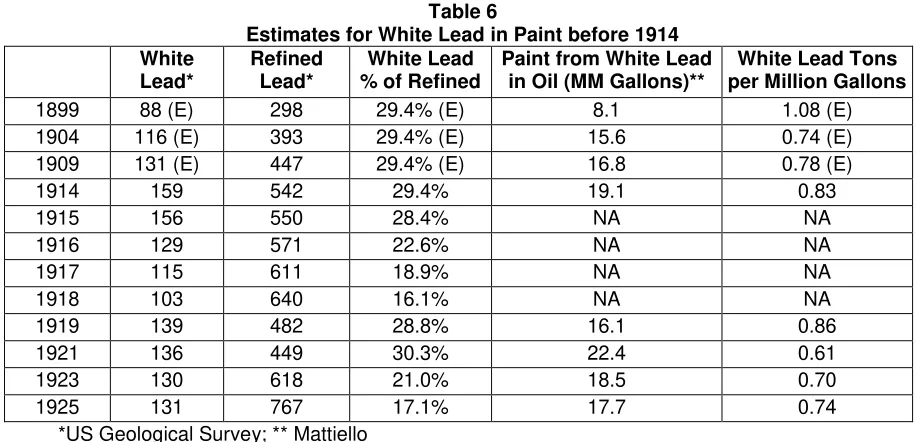
refined lead production. Table 6 shows that white lead consumption accounted for 29.4 percent

of refined lead production in 1914, and accounted for about 29 percent of refined lead production

in 1915, 1919, and 1921. White lead accounted for a much smaller share of refined lead in 1917

and 1918, but housing starts were also much lower in these two years. After 1921, the white

Therefore, this analysis assumes that white lead consumption accounted for approximately 29.4

percent of refined lead production in years prior to 1914. As a second check for this assumption,

Table 6 also shows available data on consumption of paint made from white lead in oil (Mattiello)

and shows the tons of white lead consumed per million gallons of white lead paint. This ratio

falls between .61 and .86 for years with reported data on white lead and white lead paint

consumption. The estimated white lead consumption per reported white lead paint consumption

in 1909 and 1904 are within this range, and the ratio for 1899 is just above this range.

Table 6

Estimates for White Lead in Paint before 1914 White

Lead*

Refined Lead*

White Lead % of Refined

Paint from White Lead in Oil (MM Gallons)**

White Lead Tons per Million Gallons

1899 88 (E) 298 29.4% (E) 8.1 1.08 (E)

1904 116 (E) 393 29.4% (E) 15.6 0.74 (E)

1909 131 (E) 447 29.4% (E) 16.8 0.78 (E)

1914 159 542 29.4% 19.1 0.83

1915 156 550 28.4% NA NA

1916 129 571 22.6% NA NA

1917 115 611 18.9% NA NA

1918 103 640 16.1% NA NA

1919 139 482 28.8% 16.1 0.86

1921 136 449 30.3% 22.4 0.61

1923 130 618 21.0% 18.5 0.70

1925 131 767 17.1% 17.7 0.74

*US Geological Survey; ** Mattiello

Teenage Abortions and Unwed Births

The disproportionate concentration of unwed mothers in the bottom 20 percent of the NLSY

suggests that temporal trends in unwed pregnancy may reflect trends in cognitive ability. The

time period associated with gasoline lead exposure, however, includes data from the 1950s, long

before the Roe v. Wade decision in 1973 made abortion widely available. This analysis assumes

that any cognitive deficiency associated with unwed pregnancy is associated with conception

and not with the decision to carry a child to term. Therefore, the analysis combines data on

abortion rates and unwed birth rates to create trend data for unwed pregnancies. Multiple

regression analysis was used to assess the relationship between changes in gasoline lead and

Abortion rate data were available for women ages 20-24, 18-19, and 15-17, for 1972 through

1996 (Alan Guttmacher Institute). For 1969 through 1971, data on abortion rates for all women

were used to estimate the rates for these specific age brackets (Koonin et al.). The analysis

reflects only unwed birth data for years prior to 1969 because no reliable data are available for

abortions in these years. Data on unwed birth rates were available for each age bracket over

age 15 for 1955 through 1997 (Centers for Disease Control and Prevention, 1995 and June

1998).

The abortion rate for each year was added to the unwed birth rate for the following year to create

the unwed pregnancy rate for each age bracket. The one-year lag for births recognizes that

most abortions are in the first trimester while gestation to birth is nine months. Combining

abortion and birth rates in this analysis also partially controls for the potentially important

confounding variable of changes in abortion law.

The abortion rate data report the number of abortions per thousand women in each age bracket,

whereas the unwed birth rate data report unwed births per thousand unmarried women in each

age bracket. This analysis simply adds the two rates together, because the abortion rate data for

unmarried women in specific age brackets were not available. The abortion rate data are only a

factor in years after 1968, however, and only a significant factor in years after 1973, when the

married percentage of young women was already quite low. In 1970, only four percent of

females age 15-17 and 22 percent of females age 18-19 were married. By 1979, only 16 percent

of women age 18-19 were married. Therefore, abortion rates per 1000 teenage females should

also approximate the abortion rate for unmarried teenagers. The abortion rate for women in the

20-24 age bracket will understate the abortion rate for unmarried women in this age bracket,

early twenties were married. The percent of never-married women ages 20-24 rose from 36

percent in 1970 to 50 percent in 1980 to 67 percent in 1993 (US Dept of Health and Human

Services), but married females (of all ages) account for only about 22 percent of all abortions

(Centers for Disease Control and Prevention).

Lags of 12 to 24 years were tested for gasoline lead per thousand population and the best fit lag

structure was compared with the median and mode age of unwed pregnancies in each age

bracket. The regression analysis of these data also includes a dummy variable for years after

the Roe v. Wade decision.

Abortion rate and birth rate data were also available for girls under the age of 15 for 1972

through 1997, where the population denominator used to calculate each rate is the number of

girls age 14 (Alan Guttmacher Institute). Other sources provide unwed birth rates for girls under

15 where the population denominator is the number of girls ages 10-14. This denominator

provides relatively little birth rate variation to support a regression analysis, and may obscure

trends in the age 14 population likely to dominate the under 15 abortion and birth rate data.

Also, only a very small percent of girls under age 15 were married after 1972. Therefore, the

regression analysis for girls under age 15 uses the overall birth and abortion rates for this age

bracket from 1972 through 1997, without any dummy variable for Roe v. Wade.

Covariates

The dependent variables in this analysis are measured as population rates (crime and unwed

pregnancy rates) or in other relative terms (IQ relative to population standards), as are the lead

exposure variables (gasoline and paint lead per thousand population). Therefore, potential

To evaluate potentially confounding factors affecting CogAT IQ norm comparisons, available

data were collected on temporal trends in maternal education levels, economic status, and family

demographics. Temporal trend data were available for the percentage of mothers with less than

12 years or more than 16 years education. Trends in economic status were measured by the

percentage of children living below the poverty level and below 200 percent of the poverty level.

Trends in family demographics were measured by the percentage of children living with their

mothers only. As noted above, the regression analyses for violent crime were also tested with

dummy variables for the teen and/or overall unemployment rate and the percentage of the

population in younger age brackets associated with crime.

RESULTS

Table 7 shows the change in each quartile of the blood lead distribution between NHANES II and

NHANES III Phase 1 for children under age six, and the estimated change in IQ that would result

from published estimates of the IQ to blood lead slope. The 13.1 ug/dl decline in the 25th percentile of childhood blood lead would result in an increase of 3.04 IQ points based on the

slope estimate by Schwartz (.232) for blood lead above 15 ug/dl. The 11.3 ug/dl decline in

median blood lead would result in an increase of 3.65 IQ points at the slope estimate by

Schwartz (.323) for blood lead below 15 ug/dl. The 9.8 ug/dl decline in the 25th percentile would increase IQ by 3.17 points at the Schwartz slope estimate (.323), and would increase IQ by 5.19

points at the slope estimate reported by Dudek and Merecz (.53) for blood lead at 10 ug/dl.

Table 7

Expected IQ Change due to Blood Lead Decline between NHANES II and III

NHANES II (1976-80) 1

NHANES III Phase 1 (1988-91) 1

Change (ug/dL)

IQ points per ug/dL

Expected IQ change

25th Percentile 12.0 2.2 9.8 .3232

.5303

3.17 5.19

Median 15.0 3.7 11.3 .3232 3.65

75th Percentile 19.0 5.9 13.1 .2322 3.04

1. Pirkle et al. 2. Schwartz

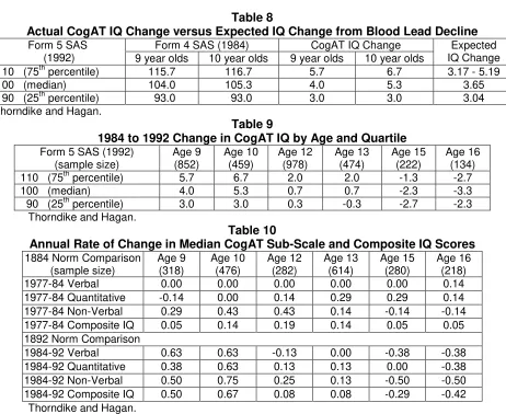
Table 8 compares the predicted change in IQ (from Table 7) with the 1992 CogAT norm

comparisons (relative to 1984) for 9 and 10 year olds with 1992 Standard Age Scores (SAS) of

110 (25th percentile), 100 (median), and 90 (75th percentile). Children ages 9 and 10 at each of these quartiles of the 1992 distribution scored substantially higher against the 1984 norm. Table

9, however, shows that the 1992 norm comparison found little change in IQ for children ages 12

and 13, and children ages 15 and 16 had substantially lower scores against the 1984 norm.

Table 10 shows the annual rate of change in CogAT subscale and composite IQ scores for

different age groups, for both the 1992 norm comparison (relative to 1984) and the 1984 norm

comparison (relative to 1977).

Table 8

Actual CogAT IQ Change versus Expected IQ Change from Blood Lead Decline

Form 5 SAS (1992)

Form 4 SAS (1984) CogAT IQ Change Expected

IQ Change

9 year olds 10 year olds 9 year olds 10 year olds

110 (75th percentile) 115.7 116.7 5.7 6.7 3.17 - 5.19

100 (median) 104.0 105.3 4.0 5.3 3.65

90 (25th percentile) 93.0 93.0 3.0 3.0 3.04

Thorndike and Hagan.

Table 9

1984 to 1992 Change in CogAT IQ by Age and Quartile

Form 5 SAS (1992) (sample size)

Age 9 (852)

Age 10 (459)

Age 12 (978)

Age 13 (474)

Age 15 (222)

Age 16 (134)

110 (75th percentile) 5.7 6.7 2.0 2.0 -1.3 -2.7

100 (median) 4.0 5.3 0.7 0.7 -2.3 -3.3

90 (25th percentile) 3.0 3.0 0.3 -0.3 -2.7 -2.3

Thorndike and Hagan.

Table 10

Annual Rate of Change in Median CogAT Sub-Scale and Composite IQ Scores

1884 Norm Comparison (sample size)

Age 9 (318)

Age 10 (476)

Age 12 (282)

Age 13 (614)

Age 15 (280)

Age 16 (218)

1977-84 Verbal 0.00 0.00 0.00 0.00 0.00 0.14

1977-84 Quantitative -0.14 0.00 0.14 0.29 0.29 0.14

1977-84 Non-Verbal 0.29 0.43 0.43 0.14 -0.14 -0.14

1977-84 Composite IQ 0.05 0.14 0.19 0.14 0.05 0.05

1892 Norm Comparison

1984-92 Verbal 0.63 0.63 -0.13 0.00 -0.38 -0.38

1984-92 Quantitative 0.38 0.63 0.13 0.13 0.00 -0.38

1984-92 Non-Verbal 0.50 0.75 0.25 0.13 -0.50 -0.50

1984-92 Composite IQ 0.50 0.67 0.08 0.08 -0.29 -0.42

Thorndike and Hagan.

Figure 2 presents temporal trend data for confounding variables that might have affected the

only and the percentage of children living in poverty both increased from 1970 to 1990, and there

was no significant change in the percentage of children living below 200 percent of the poverty

level. The percentage of mother’s with less than 12 years of education declined between 1970

and 1990, and the percentage of mothers with more than 16 years of education increased.

US Department of Health and Human Services: Trends in the Well-Being of America’s Children and Youth: 1996

US Department of Health and Human Services: Health, United States, 1995.

Violent Crime and Unwed Teen Pregnancy

Table 11 shows the regression results for the best fit lag structures associating lead exposure

with unwed pregnancy and violent crime. Table 12 compares the best-fit lag structure (highest

R2 and lowest p-value for lead) for each of these regressions with the median and mode ages of

unwed pregnant teens in each age bracket and individuals arrested in each violent crime

category. Figures 3 through 12 show a time series comparison of lead exposure per thousand

population versus the best-fit lags for each of the unwed pregnancy and violent crime categories.

Table 11

Regression Results for Unwed Pregnancy and Violent Crime

Dependent Variable

Independent

Variable Coefficient

Standard

Error p-Value R2

Teen Pregnancy Under Age 15

Intercept 8.45 0.97 .0000

.58

Lead, 15-year lag 4.97 0.89 .0000

Unwed Pregnancy Ages 15-17

Intercept -1.01 2.30 .6634

.96

Lead, 17-year lag 26.28 2.99 .0000

Roe v. Wade 22.78 1.76 .0000

Unwed Pregnancy Intercept -1.97 5.93 .7417

Figure 2

Temporal Trends in IQ Covariates (26,27)

Ages 18-19 Lead, 20-year lag 60.99 8.63 .0000 .94

Roe v. Wade 38.86 5.39 .0000

Unwed Pregnancy Ages 20-24

Intercept -2.37 5.68 .6793

.90

Lead, 24-year lag 96.14 5.88 .0000

Murder (1960-1998)

Intercept 3.40 0.62 .0000

.60

Lead, 18-year lag 4.74 0.62 .0000

Murder (1900-1998)

Intercept 527.81 725.13 .7279

.46

Lead, 21-year lag 5.98 0.66 .0000

Assault

Intercept -24.08 19.00 .2139

.89

Lead, 23-year lag 327.41 19.29 .0000

Rape

Intercept -9.73 4.32 .0306

.87

Lead, 21-year lag 29.90 2.33 .0000

Teen Unemployment 0.63 0.28 .0316

Robbery

Intercept -62.41 33.95 .0742

.79

Lead, 19-year lag 181.36 19.31 .0000

Teen Unemployment 4.45 2.30 .0603

All Violent Crime

Intercept -581.42 600.04 .3398

.90

Lead, 23-year lag 4683.36 324.21 .0000

Teen Unemployment 81.15 39.03 .0457

Table 12

Comparison of Best-Fit Lags with

Median and Mode Ages of Affected Populations

Dependent Variable Best-Fit

Lag

Age of Unwed Women and Arrests*

Mode Median

Teen Pregnancy under Age 15 15 14 14

Unwed Pregnancy Ages 15-17 17 17 17

Unwed Pregnancy Ages 18-19 20 19 19

Unwed Pregnancy Ages 20-24 24 21-23 21-23

Murder (1960-98) 18 18 – 23 23 - 29

Murder (1900-98) 21 18 – 23 23 - 29

Assault 23 18 – 24 25 - 28

Rape 21 18 – 21 22 –27

Robbery 19 17 – 18 19 - 22

All Violent Crime 23 18 – 21 22 - 26

Figure 3

Gasoline Lead Versus Teen Pregnancies: Under 15 Years Old

0 0.3 0.6 0.9 1.2 1.5 1941 :195 6 1944 :195 9 1947 :196 2 1950 :196 5 1953 :196 8 1956 :197 1 1959 :197 4 1962 :197 7 1965 :198 0 1968 :198 3 1971 :198 6 1974 :198 9 1977 :199 2 1980 :199 5 1983 :199 8 1986 :200 1

Lead Year: Conception Year (15 year lag)

T o n s o f G a s o li n e L e a d p e r T h o u s a n d Po p u la ti o n 0 2 4 6 8 10 12 14 16 Pre g n a n ci e s U n d e r A g e 1 5 p e r 1 ,0 0 0 W o m e n U n d e r A g e 1 5 Gasoline Lead Conceptions Figure 4

Gasoline Lead Versus Unwed Pregnancies: Ages 15-17

0 0.3 0.6 0.9 1.2 1.5 1941 :195 8 1944 :196 1 1947 :196 4 1950 :196 7 1953 :197 0 1956 :197 3 1959 :197 6 1962 :197 9 1965 :198 2 1968 :198 5 1971 :198 8 1974 :199 1 1977 :199 4 1980 :199 7 1983 :200 0 1986 :200 3

Lead Year: Conception Year (17 year lag)

Figure 5

Gasoline Lead Versus Unwed Pregnancies: Ages 18-19

0 0.3 0.6 0.9 1.2 1.5 1941 : 196

1

1944 : 196

4

1947 : 196

7

1950 : 197

0

1953 : 197

3

1956 : 197

6

1959 : 197

9

1962 : 198

2

1965 : 198

5

1968 : 198

8

1971 : 199

1

1974 : 199

4

1977 : 199

7

1980 : 200

0

1983 : 200

3

1986 : 200

6

Lead Year: Conception Year (20 year lag)

Figure 6

Gasoline Lead Versus Unwed Pregnancies: Ages 20-24

0 0.3 0.6 0.9 1.2 1.5 1941 : 196

5

1944 : 196

8

1947 : 197

1

1950 : 197

4

1953 : 197

7

1956 : 198

0

1959 : 198

3

1962 : 198

6

1965 : 198

9

1968 : 199

2

1971 : 199

5

1974 : 199

8

1977 : 200

1

1980 : 200

4

1983 : 200

7

1986 : 201

0

Lead Year: Conception Year (24 year lag)

T o n s o f G a s o lin e L e a d p e r T h o u s a n d P o p u la tio n 0 20 40 60 80 100 120 140 U n w e d P re g n a n c ie s : A g e s 2 0 -2 4 p e r 1 ,0 0 0 W o m e n A g e s 2 0 -2 4 Gasoline Lead Conceptions Figure 7

Gasoline Lead Versus Rape

0 0.3 0.6 0.9 1.2 1.5 1941 :196 2 1944 :196 5 1947 :196 8 1950 :197 1 1953 :197 4 1956 :197 7 1959 :198 0 1962 :198 3 1965 :198 6 1968 :198 9 1971 :199 2 1974 :199 5 1977 :199 8 1980 :200 1 1983 :200 4 1986 :200 7

Lead Year: Rape Year (21 year lag)

P ag e 36 F ig u re 9 G a s o lin e L e a d Ve rs u s A g g ra v a te d A s s a u lt

0 0.3 0.6 0.9 1.2 1.5 19 41_:1 96₄ 19₄₄ :1 96₇ 19₄₇ :1 97₀ 19 50_:1 97₃ 19₅₃ :1 97₆ 19₅₆ :1 97₉ 19 59_:1 98₂ 19 62_:1 98₅ 19₆₅ :1 98₈ 19₆₈ :1 99₁ 19 71_:1 99₄ 19 74_:1 99₇ 19₇₇ :2 00₀ 19 80_:2 00₃ 19 83_:2 00₆ 19₈₆ :2 00₉ L e a d Y e a r: A s s a u lt Y e a r (2 3 y e a r la g )

Tons of Gasoline Lead per Thousand Population

0 50 100 150 200 250 300 350 400 450 500

Aggravated Assaults per 100,000 Inhabitants

G a s o lin e L e a d A g g ra v a te d A s s a u lt Fig u re 8 G a s o lin e L e a d Ve rs u s R o b b e ry

0 0.3 0.6 0.9 1.2 1.5

19₄₁ :19 60 19 44 :19 63 19₄₇ :19 66 19₅₀ :19 69 19 53 :19 72 19₅₆ :19 75 19₅₉ :19 78 19 62 :19 81 19₆₅ :19₈₄ 19₆₈ :19 87 19 71 :19 90 19 74 :19₉₃ 19₇₇ :19 96 19 80 :19 99 19₈₃ :20₀₂ 19₈₆ :20 05 L e a d Y e a r: R o b b e ry Y e a r (1 9 y e a r la g )

Tons of Gasoline Lead per Thousand Population

0 50 100 150 200 250 300

Robberies per 100,000 Inhabitants

Figure 10

Gasoline Lead Versus Murder

0 0.3 0.6 0.9 1.2 1.5 1941 :195 9 1944 :196 2 1947 :196 5 1950 :196 8 1953 :197 1 1956 :197 4 1959 :197 7 1962 :198 0 1965 :198 3 1968 :198 6 1971 :198 9 1974 :199 2 1977 :199 5 1980 :199 8 1983 :200 1 1986 :200 4

Lead Year: Murder Year (18 year lag)

T o n s o f G a s o li n e L e a d p e r T h o u s a n d Po p u la ti o n 0 2 4 6 8 10 12 M u rd e rs p e r 1 0 0 ,0 0 0 I n h a b it a n ts Gasoline Lead Murder Figure 11

Gasoline Lead Versus Violent Crime

0 0.3 0.6 0.9 1.2 1.5 1941 :196 4 1944 :196 7 1947 :197 0 1950 :197 3 1953 :197 6 1956 :197 9 1959 :198 2 1962 :198 5 1965 :198 8 1968 :199 1 1971 :199 4 1974 :199 7 1977 :200 0 1980 :200 3 1983 :200 6 1986 :200 9

Lead Year: Crime Year (23 year lag)