BASIC BIOMEDICAL
RESEARCH
-Full Papers
Effects of White Matter Microstructure on Phase
and Susceptibility Maps
Samuel Wharton and Richard Bowtell*
Purpose:To investigate the effects on quantitative susceptibility mapping (QSM) and susceptibility tensor imaging (STI) of the fre-quency variation produced by the microstructure of white matter (WM).
Methods:The frequency offsets in a WM tissue sample that are not explained by the effect of bulk isotropic or anisotropic mag-netic susceptibility, but rather result from the local microstructure, were characterized for the first time. QSM and STI were then applied to simulated frequency maps that were calculated using a digitized whole-brain, WM model formed from anatomical and dif-fusion tensor imaging data acquired from a volunteer. In this model, the magnitudes of the frequency contributions due to ani-sotropy and microstructure were derived from the results of the tissue experiments.
Results: The simulations suggest that the frequency contribu-tion of microstructure is much larger than that due to bulk effects of anisotropic magnetic susceptibility. In QSM, the micro-structure contribution introduced artificial WM heterogeneity. For the STI processing, the microstructure contribution caused the susceptibility anisotropy to be significantly overestimated.
Conclusion:Microstructure-related phase offsets in WM yield artifacts in the calculated susceptibility maps. If susceptibility mapping is to become a robust MRI technique, further research should be carried out to reduce the confounding effects of microstructure-related frequency contributions. Magn Reson Med 73:1258–1269, 2015.VC 2014 Wiley Periodicals, Inc.
Key words:Quantitative susceptibility mapping; phase imag-ing; microstructure; white matter; anisotropy; gradient echo MRI
INTRODUCTION
Phase images of the human brain acquired at high-field strengths using gradient echo (GE) MRI show exquisite tis-sue contrast (1–4). In most studies involving GE phase imaging, it is assumed that the dominant source of phase contrast is the variation in isotropic magnetic susceptibility across different tissues (5). This assumption has led to the
development of a plethora of sophisticated techniques for inverting phase measurements to yield three-dimensional (3D) maps of the isotropic magnetic susceptibility (6–12). These “quantitative susceptibility mapping” (QSM) meth-ods take advantage of the simple, Fourier relationship con-necting the underlying distribution of isotropic magnetic susceptibility to the induced dipolar magnetic fields whose effect can be measured in phase images (13,14). Recently, however, several research groups have described additional mechanisms that could give rise to phase contrast in GE images: (i) exchange processes (15); (ii) nuclear magnetic resonance (NMR)-invisible microstructure (16); (iii) aniso-tropic magnetic susceptibility (17,18). Despite an increasing effort to quantify the contributions of each of these contrast mechanisms to phase measurements (19–23), the effect that these contributions have on susceptibility maps, calculated using QSM methods that assume isotropic magnetic sus-ceptibility is the only cause of phase variation, has not been characterized. Only by understanding the impact of the additional phase contrast mechanisms on susceptibility mapping can the true value of QSM and other related methods be fully appreciated.
There are many potential applications of QSM due to the sensitivity of susceptibility maps to a range of endogenous biomarkers such as myelin (24,25), calcification (26), and iron content (8,27). A recent postmortem study showed that the measured isotropic susceptibility correlates well with iron content in deep gray matter (GM) structures (28), but the correlation between iron and susceptibility in white matter (WM) is weak. One explanation for the weak correla-tion in WM is the confounding contribucorrela-tion of other phase contrast mechanisms. In 2008, Zhong et al. (15) suggested that chemical exchange between water molecules and pro-teins could induce a local shift in the resonant frequency that affects the phase difference measured between GM and WM. In 2009, He and Yablonskiy (16) proposed that biased sampling of the magnetic field on the microscopic scale, due to the presence of NMR-invisible oriented microstruc-ture, could lead to local frequency offsets that do not reflect the local magnetic susceptibility, while Marques et al. (29) showed that isotropic susceptibility could not fully explain WM phase contrast in an ex vivo murine brain. In 2010, Lee et al. (18) used measurements on fixed, postmortem tis-sue samples to show that the magnetic susceptibility of WM has a measurable anisotropy. Around the same time, Liu (17) showed that the full anisotropic magnetic suscepti-bility tensor can be reconstructed by solving the relevant inverse problem, provided that measurements of the field perturbation with the anisotropic susceptibility distribution oriented at a sufficient range of different orientations to the main magnetic field are available. This “susceptibility Sir Peter Mansfield Magnetic Resonance Centre, School of Physics and
Astronomy, University of Nottingham, University Park, Nottingham, United Kingdom.
*Correspondence to: Richard Bowtell, Sir Peter Mansfield Magnetic Reso-nance Centre, School of Physics and Astronomy, University of Nottingham, University Park, Nottingham NG7 2RD, United Kingdom. E-mail: Richard. [email protected]
Additional Supporting Information may be found in the online version of this article.
Received 16 September 2013; revised 23 January 2014; accepted 3 February 2014
DOI 10.1002/mrm.25189
Published online 11 March 2014 in Wiley Online Library (wileyonlinelibrary. com).
Magnetic Resonance in Medicine 73:1258–1269 (2015)
tensor imaging” (STI) method has been applied to phase images acquired at multiple orientations to the field from postmortem mouse brain (17), and more recently from the human brain in vivo (30).
Recent studies have suggested that the source of the ani-sotropic susceptibility of WM is the myelin sheath (19,30– 32). This is composed of multiple lipid bilayers in which the lipid chains are radially oriented with respect to the approximately cylindrical sheath. The magnetic suscepti-bility in the myelin sheath is consequently described by a cylindrical symmetric tensor in which the principal axis is radially oriented. This geometry means that average mag-netic susceptibility in a voxel containing multiple aligned nerve fibers is anisotropic because of the different average magnetic properties perpendicular and parallel to the fibers, but more interestingly the radial anisotropy in the myelin sheath also produces average frequency offsets of different polarity in the nerve sheath and lumen, whose magnitudes depends on the fiber geometry and orientation to the applied B0-field (19). As a result of the low water content of myelin and the rapid T2*-decay of the myelin water signal (33), the GE phase is more sensitive to the average frequency offsets inside the nerve lumens and in extraaxonal regions than to the offset in the myelin sheath. This gives rise to local frequency=phase offsets which are sensitive to the local WM microstructure (19,20,34).
The frequency contribution of microstructure was explored in a recent study by Luo et al. (22). These authors recorded frequency data from a rat optic nerve sample at multiple orientations to the main magnetic field and showed that there was a significant mismatch between measured frequency values and expected values based on a simple isotropic susceptibility model. Due to the experimental design utilized by Luo et al., it was not possible for them to estimate the anisotropic susceptibil-ity of the WM sample. Here, we build upon this previous work and use a somewhat similar experimental setup to characterize the isotropic and anisotropic susceptibility and microstructural effects in a WM tissue sample.
In this study, we investigate the effects of susceptibility anisotropy and WM microstructure on QSM data. First, the isotropic and anisotropic magnetic susceptibility of a fresh sample of postmortem WM with known fiber orientation was quantified by comparing the measured external field variation with the sample at multiple orientations to the main magnetic field to field simulations. By subtracting the simulated WM frequency maps from the measured frequency maps, maps of the residual frequency offsets were formed. Inspection of the fiber-orientation dependency of these resid-ual WM frequency offsets allowed the microstructure contri-bution to be characterized and separated from the unknown exchange contribution. Simulations were then carried out to investigate the effect of frequency offsets due to anisotropy and microstructure on QSM-based calculations of isotropic magnetic susceptibility. In addition, the artifacts caused by microstructure in STI processing were also investigated.
METHODS
White Matter Sample Preparation
Optic nerve forms an ideal structure for investigating phase offsets due to WM (22) because it forms a compact
cylindri-cal structure containing many nerve fibers that are aligned with the axis of the optic nerve. Here, a section of optic nerve of around 0.4-cm diameter was harvested from a recently euthanized 60 kg pig and trimmed to a length of approxi-mately 2 cm. The nerve section was embedded in agar (1.5% agarose gel made from 1% saline solution) contained in a Perspex sphere of 10-cm diameter. Imaging was carried out about 4 hours after the sample had been harvested.
Image Acquisition
Images were acquired on a Philips Achieva 7T scanner (Philips Medical Systems, Best, the Netherlands) using a 32-channel receiver head coil. A dual-echo, 3D, spoiled GE sequence was used to image the spherical tissue phantom with parameters: repetition time (TR)¼ 28 ms; echo time (TE)1 ¼ 7 ms; TE2 ¼ 20 ms; field of view (FOV)¼112112 70 mm3; flip-angle¼ 11o; scan time
¼15 min; isotropic resolution¼ 0.5 mm; unipolar read-out gradients. The tissue phantom was imaged with the optic nerve section oriented at 10 different angles to the B0-field, This resulted in 10 data sets in which the angle, u, between the nerve axis andB0,varied between 0and 90 in approximately even steps of 10. The total
scan-ning time was approximately 200 min. The first two image data sets were acquired with the nerve parallel (u¼ 0) and then perpendicular (u¼ 90) to B
0,while the order of subsequent acquisition was randomized in order to reduce any systematic errors due to tissue degradation over the course of the experiment.
A single healthy human subject of 28 years of age was also imaged at 7T (with informed consent and local ethical approval) using the same GE sequence as was used in the phantom experiments (see parameters above), but with a coarser isotropic resolution of 1 mm and at a single orien-tation. In addition, diffusion tensor imaging (DTI) data was acquired (sequence parameters: TE¼57 ms; TR¼8.6 s; FOV¼224224 104 mm3, in-plane resolution¼2 mm; slice thickness¼2 mm; scan time¼7 min; 32 diffu-sion gradient directions, b-value¼1000 s mm-2) and T1-weighted anatomical images (sequence parameters: TE¼
3.7 ms; TR¼8 ms; inversion time [TI]¼960 ms; long-TR
¼2.8s; turbo field echo (TFE) factor¼205; flip angle¼8o; FOV¼ 256 256 160 mm3; isotropic resolution ¼ 1 mm) of the same subject were acquired at 3T.
Image Processing
The phase data from each echo were unwrapped using a fast 3D method (35). Frequency maps were formed by taking the difference of the unwrapped phase values associated with the first and second echoes and then scaling the result by the TE-difference (DTE ¼13ms). Similarly,R
2 maps were formed from the dual-echo data
by dividing the difference in the natural logarithm of the magnitude data associated with each TE by DTE. The magnitude images associated with the second echo of each of the 10 different data sets were coregistered using a rigid body transform in FMRIB’s Linear Image Registry Tool (36) to a common sample space, in which the nerve fibers in the optic nerve section were aligned with thez -axis. The resulting rotation matrices were then applied to the associated frequency andR
maps were spatially filtered to remove unwanted back-ground fields using the sophisticated harmonic artifact reduction for phase data (SHARP) method (8). The DTI data were processed using FSL dtifit (37) to yield maps of the fractional anisotropy (FA), and of the eigenvectors describing the fiber orientations.
Calculation of Susceptibility From External Field
In standard susceptometry experiments, the known form of the external field perturbation due to a sample of spe-cific geometry (e.g., an infinite cylinder perpendicular to B0) is compared to measured field data in order to calcu-late the relative isotropic magnetic susceptibility offset of the sample relative to the reference medium in which it is embedded (38). As shown by Lee et al. (18), this methodology can be extended to allow for calculation of the anisotropic magnetic susceptibility of a small fixed WM tissue sample. This approach is advantageous because by focusing on the external field perturbation it eliminates any sensitivity to exchange or microstructure, which only produce signal changes within the sample. In this study, we adopt a similar approach for calculating susceptibility based on measurement of the field varia-tion induced outside the fresh tissue sample.
The simulated frequency map, fsim, due to a sample
embedded in a reference medium can be written as
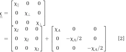
fsim¼xIgDBIþxAgDBA [1]
where xI and xA are scalar values describing the
iso-tropic and anisoiso-tropic components of a cylindrically symmetric susceptibility tensor (19),x, representing the
magnetic properties of the sample relative to the sur-rounding medium such that
x ¼
xjj 0 0
0 x? 0
0 0 x?
2 6 6 4 3 7 7 5 ¼
xI 0 0
0 xI 0
0 0 xI
2 6 6 4 3 7 7 5þ
xA 0 0
0 xA=2 0
0 0 xA=2
2 6 6 4 3 7 7 5 [2]
where xjj and x?are the magnetic susceptibility of the
sample parallel and perpendicular to the principal axis of the cylindrically symmetric susceptibility tensor. DBIand DBA in Equation [1] represent the field
perturba-tions per unit of isotropic and anisotropic magnetic sus-ceptibility, and are given by:
DBI ¼B0IFTfFTðMÞ ð1=3-cos2ukÞg [3]
DBA¼
B0
4 IFT
FTð3Msin 2ucosfÞ ðsin 2ukcosfkÞ=2
þFTð3Msin 2usinfÞ ðsin 2uksinfkÞ=2
þFTMð1þ3 cos 2uÞ ðcos2u
k1=3Þ
8 > > > < > > > : 9 > > > = > > > ; [4]
Here, uk and fk are spherical polar coordinates in
k-space, with thez-axis aligned with the direction ofB0,
u, and f are spherical polar coordinates describing the direction of the principal axis of the susceptibility tensor (defined as thex-axis in Eq. [2]) relative to theB0 direc-tion and FT (IFT) denotes a 3D (inverse) Fourier trans-form. The shape of the sample is represented by the digitized mask function,M, which takes a value of 1 in voxels lying within the sample and a value of 0 in voxels in the surrounding reference medium. Equation [3] is the standard Fourier representation of the field perturbation due to a 3D distribution of isotropic magnetic suscepti-bility (13,14). The derivation of the Fourier expression in Eq. [4], which can be used to calculate the field due to a zero-trace, cylindrically symmetric susceptibility tensor is described in our previous work (19,39). For this approach to be valid, the sample must have homogenous magnetic properties: That is, the values ofxI andxA, as well as the
[image:3.612.91.303.466.554.2]direction of the principal axis of the susceptibility tensor, must be uniform over the entire sample. The sample used in this study should satisfy these conditions because the direction of the nerve fibers, and the extent to which these nerve fibers are myelinated, is expected to be fairly uniform over a short section of optic nerve.
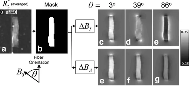
Figure 1 shows the steps used to simulate the fre-quency map due to the optic nerve sample. A 3D mask of the WM sample (see Fig. 1b),M, was drawn based on aR
2 map (Fig. 1a) formed by averaging theR2 data from
all sampling orientations. By substituting the sample mask into Eq. [3] and Eq. [4], the isotropic and aniso-tropic field perturbations maps were separately simu-lated for each of the 10 sampling orientations. As part of these calculations, the spherical polar coordinates in Eq. [3] and Eq. [4] had to be recalculated based on the direc-tion of B0 for each sampling orientation. Representative slices of the simulated DBI and DBA field maps are
shown in Figure 1c to 1h for three different orientations. Least-squares fitting of the simulated frequency values in the region outside the mask to experimental measure-ments for all sample orientations was then used to esti-mate the values of xI and xA in the WM sample. The simulated frequency maps were spatially filtered using SHARP in an identical manner to the measured fre-quency data before the fitting was carried out. Only vox-els external to the sample mask were included to avoid the confounding local effects of exchange and micro-structure. The external region was defined by dilating the sample mask by 8 voxels in all dimensions followed by subtraction of the original sample mask dilated by 1 voxel. Also, to avoid including erroneous field values due to the presence of air-bubbles in the agarose gel, only voxels with R
2 less than 15 s1 were included in
the fitting procedure, which was carried out using the “lscov” function in MATLAB 7.5.0 (MathWorks, MA, U.S.A.). This utilizes matrix inversion based on orthogo-nal decomposition. As this was a matrix inversion-based procedure, it was not necessary to define a fitting range, and the fitted values should yield a global minimum in the least-squares residual.
Measuring residual frequency values
resulting simulated frequency maps from the measured frequency maps, a map of the residual frequency offset, fR, was formed at each sampling orientation. The fR
-maps represent the measured frequency offsets that are poorly explained by the bulk isotropic and anisotropic susceptibility effects described by Eqs. [3] and [4]; there-fore, they are likely to be dominated by contributions from the exchange and microstructure mechanisms local to the WM sample. To investigate this hypothesis, thefR
offset inside the optic nerve sample was measured by averaging over an ROI defined by eroding the mask, M, by 1 voxel. This was repeated for all sampling orienta-tions to yield 10 averagefRmeasurements.
The residual frequency,fR, is expected to vary withuas:
fR¼Asin2uþb [5]
where A characterizes the amplitude of the variation in fR on rotating the sample, andbis au-independent offset.
The form of Eq. [5] is based on the assumption that the amplitude of the microscopic field variations due to myelinated nerve fibers, which underlie the microstruc-ture contrast mechanism, varies as sin2u (16,19,31,34).
The measured fR-values were fitted to Eq. [5] to yield estimates ofAand b. As exchange processes are insensi-tive to fiber orientation, A is expected to be solely dependent on microstructure effects. In contrast, b is likely to contain contributions from both exchange and microstructure (19).
Simulating whole brain frequency maps
To investigate the effect of frequency offsets due to microstructure on QSM and STI, the frequency varia-tions produced by a digitized model of the human brain were calculated. To generate the model, FMRIB’s Auto-mated Segmentation Tool (40) was first used to segment the T1-weighted anatomical brain image acquired from a single healthy subject, yielding digitized masks of WM and non-WM tissue (cerebrospinal fluid [CSF] and GM). As the focus of this study is the effect of WM microstruc-ture on QSM and STI, the values of xI and xA in CSF
and cortical GM were set to zero. The xI and xA values
used in the WM regions were based on the results of the optic nerve experiments. The estimates ofxA and the
fit-ted microstructure-relafit-ted amplitude parameter, A, are absolute measures and are likely to manifest in human WM with similar values to those measured in the por-cine optic nerve sample. However, the estimates of xI
and the u-independent residual frequency offset, b, are relative measures that depend on the isotropic magnetic susceptibility and any exchange-related frequency offset in the media surrounding the WM. For the tissue phan-tom, the reference medium is agarose gel, but in the human brain, WM is mostly surrounded by GM. As there is insufficient data in the literature to form a robust esti-mate of the exchange-based frequency offset in GM rela-tive to WM, a single u-independent residual frequency offset was not included in the simulations. In contrast, sufficient literature now exists to suggest that WM has a diamagnetic isotropic susceptibility offset of the order of
0.05 ppm relative to GM (8,19,24). The simulations were, therefore, carried out with the value of xI in WM set to0.05 ppm relative to that in non-WM.
In addition to WM and cortical GM, iron-rich deep GM structures in the basal ganglia region can make large con-tributions to frequency maps acquired in vivo (4,5,7,8,10,11). In an effort to simulate these additional frequency offsets, masks of several deep GM regions were hand-drawn on the magnitude data associated with the second echo of the GE data set to yield 3D binary masks that could be populated with susceptibility values. The chosen structures were the globus pallidus (GP), putamen (PU), caudate nucleus (CN), thalamus (TH), and pulvinar part of the thalamus (PV). For each region, the xI value
relative to the surrounding WM was based on recent liter-ature (7,8,41): GP ¼ 0.15 ppm, PU ¼ 0.05 ppm; CN ¼
0.05 ppm; TH ¼ 0.00 ppm; PV ¼ 0.03 ppm. Only iso-tropic susceptibility effects were considered because these iron-rich structures are not thought to exhibit strong ani-sotropy- or microstructure-related effects.
[image:4.612.145.471.76.224.2]The frequency variation, fI, due to the isotropic sus-ceptibility of the WM and deep GM structures in the FIG. 1. Steps followed in generating simulated field maps. The averageR
2map (average over all 10 sample orientations) (a) was used
brain model, was calculated using Eq. [3], with the WM and deep GM masks, multiplied by their respective xI
-values, taking the place ofM. To calculate the frequency variation due to the anisotropic susceptibility of WM, it is necessary to know the average fiber direction in each voxel, which dictates the direction of the principal axis of the susceptibility tensor. This information was derived from the DTI data and then used to evaluate the values of h and u, which characterize the average fiber orientation relative to the B0-field in each voxel. These values were fed into a modified version of Eq. [4], in which the maskMwas replaced by the WM mask multi-plied by a spatially varying value ofxA in order to calcu-late the frequency variation, fA, produced by the anisotropic susceptibility of the WM in the brain model. We allowed the value ofxAto vary in order to reflect the variation of the coherence of fiber orientations in voxels in different WM regions. For example, the fiber orienta-tions are expected to be fairly uniform in a voxel in the corpus callosum (CC), but are likely to have a greater dis-persion in voxels located in cortical white matter. As the magnitude of the anisotropy of the susceptibility tensor in a WM voxel is expected to be linked to the dispersion of fiber orientations, we modulated the magnitude ofxA
used in the simulations based on the FA measured from the DTI data. The FA values were normalized by divid-ing by a scaldivid-ing factor 0.59 based on a literature value for the in vivo FA of the human optic nerve tissue (42). To simplify the simulations, FAnorm was set to zero in
the segmented deep GM structures. The resultingFAnorm
values were multiplied by the xA value estimated from
the optic nerve experiments to yield a spatially varying xA map, in which the local magnitude depends on the
local FA estimated from the DTI experiment.
A spatially varying microstructure-related frequency offset,fM, was also calculated using
fM ¼Aðsin2u2=3ÞFAnormþC [6]
where A is the amplitude calculated from the fR-values
measured in the optic nerve, u is the angle between B0 and the fiber orientation, which was derived from the DTI data, andCis au-independent frequency offset. In a similar manner to the formation of thexA-map,FAnormis
included in Eq. [6] to generate a more realistic distribu-tion of the magnitude of the microstructure offset. The factor of2=3 was included in Eq. [6] to ensure that the average offM over a random distribution of fiber
orienta-tions is equal to zero. By definingfM in this manner, the
average effect of fM is more easily separable from the
unknown,u-independent frequency offset represented by C. C is included in Eq. [6] to model local exchange-induced,u-independent frequency offsets in WM (15), as well as u-independent WM frequency shifts due to microstructure (19,20,23,34). Previous work by our group (19) and others (15,21,43) has suggested that there are exchange-related frequency offsets on the order of 0.01ppm in WM relative to GM, which at 7T corresponds to a frequency offset of 3Hz. To investigate the effects of including a range of u-independent WM-GM offsets, frequency maps were simulated with C set to 3Hz, 0 Hz, andþ3Hz. For consistency with the data from the in
vivo experiments, where no frequency information is available outside of the brain, the simulated frequency maps were masked, using the mask produced by apply-ing FMRIB’s Brain Extraction Tool (44) to the T1-weighted anatomical data.
Investigating Artifacts in QSM
In this study, QSM was carried out using the thresholded k-space division (TKD) method (9,45). This method was chosen due to its speed and simplicity. To assess the effect of the frequency offsets due to anisotropy and microstructure on the calculated susceptibility maps, TKD-based QSM was applied to three different frequency maps: (i) a frequency map due to purely isotropic suscep-tibility offsets,fI; (ii) a frequency map containing isotropic
and anisotropic contributions,fIþfA; and (iii) a frequency
map containing susceptibility and microstructure related contributions,fIþfAþfM. In these simulations,C (in Eq.
[6]) was set to zero (fMðC¼0Þ). The TKD kernel threshold
was set equal to 0.07, which corresponds to a truncation value of 14 in the reciprocal units proposed by Shmueli et al. (9). This value was chosen through trial and error as a good compromise between contrast and artefact-related noise (9). In an additional experiment, the fully relaxed TKD kernel proposed in recent work (45) was also applied to thefIþfAþfMðC¼0Þ data set. As part of the TKD
proc-essing, a global correction factor was applied to compen-sate for the underestimation of susceptibility values due to kernel truncation (45). Difference from truth (DFT) maps were formed by subtracting the xI map (including
WM and deep GM offsets) used in the simulations from the calculated susceptibility maps.
Investigating Artifacts in Susceptibility Tensor Imaging
The effects of microstructure-related frequency offsets on STI were also investigated. fI,fA, and fMðC¼0Þ data were
simulated, as described above, but for 16 different orien-tations ofB0with respect to the sample. These directions were chosen so that the tips of the B0 vectors approxi-mately were spread evenly over a hemispherical surface. This is equivalent to rotating the sample in the field of the scanner in order to properly condition the ill-posed inversion problem underpinning STI (17). In a similar manner to the QSM experiments, STI was separately applied tofIþfA data andfIþfAþfMðC¼0Þ data. The STI
data processing was carried out according to Liu (17), with a limit of 30 iterations imposed upon the conjugate gradient minimization algorithm. All QSM and STI proc-essing was carried out in MATLAB using a 64-bit Linux system with a 2 GHz dual core AMD processor and 8 GB of RAM. The eigenvalues, (x1;x2;x3), and eigenvectors of the resulting susceptibility tensors were calculated at each voxel (17). The reconstructed isotropic and aniso-tropic susceptibility values are then given by
xI ¼ ðx1þx2þx3Þ=3 [8]
xA¼x1xI [8]
with x1, represents the estimated fiber direction. DFT maps were formed by subtracting the true xI and xA
maps from the reconstructed susceptibility maps based on the fIþfA and fIþfAþfMðC¼0Þ data. DFT maps were
also formed for the reconstructed V1 data by voxelwise
calculation of the magnitude of the angle between the reconstructed V1 vector and the direction of the VDTI
vector, used to simulate the fiber orientation.
[image:6.612.63.298.72.253.2]RESULTS
Figure 2 shows the results of the tissue phantom experi-ments. The best-fitting values forxI andxA, based on the external frequency variation inf (1st row in Fig. 2), were found to be 0.08152 6 0.00006 ppm and 0.01128 6 0.00009 ppm, where the quoted errors are the estimated standard errors in the least-squares fitting procedure and take into account the large number of voxels that were sampled. The correlation between DBI and DBA was
fairly low (R¼ 0.318), suggesting that the fitting proce-dure was reasonably robust. Maps of the simulated fre-quency, fsim, generated by substituting the fitted xI and xA values into Eq. [1] are also shown in Figure 2 (2nd row), along with the maps of the variation of the residual frequency offset,fR¼f fsim (3rd row in Fig. 2). ThefR
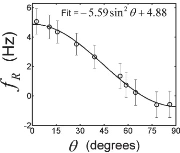
values inside the optic nerve are significant and positive for small u values, decreasing in magnitude as u increases toward 90. Figure 3 shows the variation with
u of the average value offR inside the optic nerve. The
curve described in Eq. [5] provides an excellent fit to the measured, average fR-values, yielding coefficient values
ofA5 5.596 0.12 Hz andb 54.88 6 0.07 Hz. The fit
was also carried out using onlyDBI (i.e., ignoring
anisot-ropy), which yielded axI value of0.08369860.00006
ppm and also produced average residual frequency off-sets that were well modeled by Eq. [5] with coefficient values A5 6.53 6 0.12 Hz and b 5 5.97 6 0.07 Hz. The results of an F-test suggested that, after taking into account the increased number of fitting parameters, the incorporation of xA significantly improved the fit (P <
0.001). The importance of including a xA component is further demonstrated in Suppl. Figure 1, which shows a comparison of the residual frequency offsets in the exter-nal agarose compartment for the two different forward models.
Figure 4 shows representative axial slices at the level of the optic radiations drawn from the data sets that were used in calculating the whole brain frequency maps. Figures 4a and 4d show xI and xA maps, respec-tively. ThexA-map was formed by multiplying theFAnorm
map (Fig. 4b) by the xA-value measured in the optic nerve (0.011 ppm). The principal axis of the susceptibil-ity tensor in each voxel was aligned with the principal axis of the diffusion tensor, defined by unit vector,VDTI
(Fig. 4c).
Figure 5 shows calculated frequency maps for the same axial slice shown in Figure 4. For comparison, the corresponding slice of the frequency map measured in vivo at 7T, finvivo, is also displayed (Fig. 5h). The fA
maps (Fig. 5b) show much greater heterogeneity in WM compared with the fI data (Fig. 5a), with offsets that
reflect the underlying orientation of the susceptibility tensor (see Fig. 4c). Arrows highlighting the internal cap-sule (yellow arrow), where the local WM fiber orienta-tion is parallel to B0, and the splenium (red arrow), where the local WM fiber orientation is perpendicular to B0, are shown in all images. Comparison of Figures 5a and 5b indicates that the frequency offsets produced by the anisotropic susceptibility (61 Hz) are significantly smaller than those produced by the isotropic susceptibil-ity (66 Hz). This is a consequence of the relatively small magnitude ofxA, which took a maximum value of 0.017
ppm compared to WMxI-value of 0.05 ppm. The posi-tive isotropic susceptibility of the deep GM structures FIG. 2. Results of the tissue phantom experiments. Coregistered
frequency maps (f) are shown for all 10 fiber orientations. The dipolar nature of the external field perturbation due to the optic nerve section and its rotation as the direction of B0 changes is evident from the measured frequency maps. The corresponding simulated frequency maps (fsim), based on a best fit to the
exter-nal frequency variations in f, are also shown. The residual fre-quency maps (fR) are generated by subtractingfsimfromf at each
orientation. The residual frequency offsets in the agarose gel sur-rounding the sample are small, suggesting that the measured external field variations are well characterized by the simulation. Also, a subtle line can be seen in thefRmaps showing the layer
of gel that was allowed to cool and harden to support the sample.
FIG. 3. Plot of the average residual frequency (fR) values inside
[image:6.612.342.522.553.706.2]introduces negative offsets in the surrounding WM in this axial slice through thefI-map, with particularly
neg-ative offsets associated with the internal capsule region (yellow arrow in Fig. 5a). ThefMðC¼0Þmap shows similar
heterogeneity in WM to the fA map, but the variations
are much larger, with frequency offsets in the range of 64 Hz. Figure 5d shows the composite fIþfA map and
Figure 5e to 5g shows composite maps formed by
includ-ing the microstructure-related frequency offset with three different C-values: C ¼ 3 Hz (fIþfAþfMðC¼3Þ);C ¼ 0
Hz (fIþfAþfMðC¼0Þ);C ¼3 Hz (fIþfAþfMðC¼3Þ).
[image:7.612.148.470.73.198.2]Compar-ison of these maps with Figure 5h indicates that the composite maps that incorporates the effect of micro-structure (Fig. 5e–5g) are generally more similar to the measured frequency map. In particular, they exhibit neg-ative frequency offsets in the splenium and optic FIG. 4. Representative axial slices at the level of the optic radiations of the data sets used to carry out whole brain frequency simula-tions.(a)Isotropic susceptibility map,xI, based on a segmented white matter image from a T1-weightted anatomical image. The deep
GM regions included in the isotropic model are also labeled: GP¼globus pallidus; PU¼putamen; CN¼caudate nucleus; TH¼ thala-mus; PV¼pulvinar part of the thalamus.(b)DTI-based FA map divided by estimated FA in optic nerve (0.59) to yield a normalized FA-map,FAnorm, which should be a good indicator of fiber anisotropy.(c)Colour-coded fiber-orientation map (red¼left-right, green¼
ante-rior–posterior, blue¼foot–head) based on the principal eigenvectors (VDTI) extracted from a DTI dataset. Fiber orientation information
was used in calculatingfAand fM. (d)Map of the anisotropic susceptibility, formed by multiplying the normalized FA map (b) by the
experimentally measured values of the anisotropic susceptibility of WM in the optic nerve (xA¼0.0113 ppm).
FIG. 5. Representative axial slices of simulated frequency data.(a)Simulated frequency map due to the isotropic magnetic susceptibility distribution,fI.(b)Simulated frequency map due to the anisotropic magnetic susceptibility distribution,fA.(c)Simulated frequency map
due to microstructure,fMðC¼0Þ.(d)Composite frequency map including frequency shifts due to isotropic and anisotropic magnetic
sus-ceptibility,fIþfA. Composite frequency map including frequency shifts due to isotropic and anisotropic magnetic susceptibility, as well
as microstructure with three different u-independent offsets (see C in Eq. [6]): (e) composite frequency map with C ¼ þ3 Hz, fIþfAþfMðC¼3Þ;(f)frequency map withC¼0 Hz,fIþfAþfMðC¼0Þ;(g)frequency map withC¼ 3 Hz. For comparison, an in vivo
fre-quency map,finvivo, acquired at 7T is also shown (h). The arrows in all images highlight the frequency contrast in the splenium (red
[image:7.612.145.471.408.658.2]radiations that better match the observedfinvivofrequency
behavior compared to the rather low contrast of the fI þfAimage (see red arrows). Of the three composite maps
that include the effect of microstructure, the highest level of agreement between simulations and measured values is observed for the negative C-value (fIþfAþfMðC¼3Þin Fig. 5g).
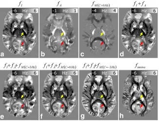
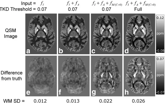
Figure 6 shows the results of the QSM calculations for the same axial slices as used in Fig. 4 and Fig. 5. The standard deviation (SD) of thexI-values in WM was
cal-culated for each dataset to provide an indication of the error in the calculated susceptibility maps; and the val-ues are listed in Figure 6. The susceptibility map calcu-lated from the fI-data (Fig. 6a) exhibits fairly
homogenous diamagnetic WM contrast (SD ¼ 0.012 ppm), and the associated DFT image (Fig. 6e) shows there are only small differences that result from the replacement of data by constant values in a small region of k-space in the TKD method. The susceptibility map calculated fromfIþfA (Fig. 6b) has a similar appearance
to the map derived from fI alone, but it exhibits a
slightly increased level of artefactualxI-variation in WM
(SD ¼ 0.013 ppm). The susceptibility map calculated fromfIþfAþfMðC¼0Þ using a TKD threshold of 0.07 (Fig.
6c) shows increased heterogeneity in WM (SD ¼ 0.022 ppm) relative to the maps produced from thefIþfA orfI
data. The associated DFT image (Fig. 6g) clearly shows that thefMðC¼0Þfrequency offsets (Fig. 5c) propagate into
the final QSM image as artefacts. From a qualitative per-spective, the susceptibility map calculated from fIþfA þfMðC¼0Þ using a fully relaxed TKD kernel (Fig. 6d)
appears to show reduced artefact levels and clearer boundaries relative to the map calculated from the same data using a TKD threshold of 0.07 (Fig. 6c). However, this qualitative improvement comes at the cost of a gen-eral increase in WM heterogeneity (SD ¼ 0.026 ppm),
also clearly shown in the associated DFT image (Fig. 6h). For comparison, the standard deviations of the frequency values in WM for fI, fA, and fMðC¼0Þ (see Fig. 5) were
found to be 3.14 Hz=0.011 ppm, 0.34 Hz=0.001 ppm, and 1.02 Hz=0.003 ppm, respectively.
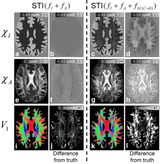
Figure 7 shows the results of the investigation of the effect of frequency offsets due to microstructure on STI. The left-hand and right-hand sides of Figure 7 show the results of applying the STI processing to the compositefI þfA and fIþfAþfMðC¼0Þ data. The representative axial
slices shown here lie at the level of the CC. The recon-structed xI (Fig. 7a), xA (Fig. 7e), and V1 (Fig. 7i) maps
calculated from the fIþfA frequency data are generally
in excellent agreement with the ground truth maps (Fig. 4), as evidenced by the low associated DFT values (Figs. 7b, 7f, and 7j). Despite this general agreement, some small errors inherent to the STI processing can be seen in the DFT image associated with the xA-map (Fig. 7f).
To probe these discrepancies further, an ROI was drawn in the CC. The average value of xA in this region of the
model used in the simulations was found to be 0.0116 0.003 ppm. Here, the error is the standard deviation over the ROI, which reflects the spatial variation ofxA in the model due to variation of theFAnormterm used in its
cal-culation (see Eq. [6] in simulating whole brain frequency maps in Methods). The average value of xA in the CC
ROI applied to the map derived from thefIþfA data was
0.01360.004 ppm, which is a factor of 1.18 times larger than the ground truth. The mean angle between the V1
vectors calculated from thefIþfAdata and theVDTI
vec-tors, which defined the direction of the principal axis of the susceptibility tensor in the model data, was 18617o in WM. In contrast to thefIþfA results, the xI, xA, and
V1 maps calculated from thefIþfAþfMðC¼0Þdata, which
[image:8.612.145.470.73.277.2]include the effect of microstructure (Fig. 7, right-hand side) show considerable errors when compared to the FIG. 6. Representative slices showing the results of the QSM calculations. The figure shows susceptibility maps produced by applying TKD-based QSM with a truncation threshold of 0.07 tofI(A),fIþfA(B), andfIþfAþfMðC¼0Þ(C) data. The susceptibility map generated
by applying the fully relaxed TKD method to thefIþfAþfMðC¼0Þ data is also shown(d). Difference from truth (DFT) images, generated
by subtracting the isotropic susceptibility map used in the model (see Fig. 4a) from each calculated susceptibility map, are also shown
original model data, as evidenced by the large offsets in the DFT images. In particular, the large positive offsets in the DFT image associated with the reconstructedxA map
(Fig. 7h) suggest that the anisotropy in WM is strongly overestimated in these data. This is also apparent from the average value ofxA in the CC ROI, which is 0.0306 0.010 ppm, that is, a factor of 2.8 times larger than the value in the model data. The generally positive offset in WM regions of the DFT image associated with the recon-structed xI map (Fig. 7d) also suggests that STI based on the fIþfAþfMðC¼0Þ data underestimates the diamagnetic
isotropic susceptibility of WM. The mean angle between the V1 vectors calculated from the fIþfAþfMðC¼0Þ data
and the VDTI vectors was larger than for thefIþfA data,
taking an average value of 28623oin WM voxels.
DISCUSSION
The fitted xA value of 0.011 ppm in the optic nerve experiments corresponds to an overall susceptibility ani-sotropy of Dx¼xjj-x?¼3xA=2¼0.017 ppm. This is larger than the Dx ¼ 0.012 ppm value estimated by Lee et al. (18), who applied a similar approach to a fixed, postmortem human CC sample. The discrepancy could be due to fixation effects because, unlike Lee et al.’s sam-ple, our sample was not fixed; but the discrepancy could also be due to differences in tissue degradation. Our sample was scanned only 4 hours after harvesting, while the time between harvesting and fixation for a human sample is likely to be significantly longer. The xI value
[image:9.612.58.386.76.412.2]of 0.082 ppm measured here suggests that WM is dia-magnetic relative to agarose gel, and this value is similar to the0.116 ppm value measured by Luo et al. (22) in a rat optic nerve using a similar approach, but with forma-lin as the reference medium. These results add to the growing body of evidence suggesting that WM is diamag-netic relative to water. The average residual frequency inside the optic nerve sample varied by 5.59 Hz as the nerve orientation was rotated from parallel to perpendic-ular to the field, showing a sin2u dependence on the angle of the nerve to the field that is consistent with the predicted effect of WM microstructure (16,19,31). Using a forward model that only incorporated bulk isotropic susceptibility, Luo et al. (22) also measured a similar orientation-dependent frequency offset that, after conver-sion into Hz at 7 T and adopting the sign conventions used in our work, would yield approximate coefficients ofA ¼ 6.7 Hz andb ¼ 4.5 Hz in Eq. [5]. These values are of the same sign and of a similar magnitude to the microstructure-related offsets measured here using a purely isotropic model (A ¼ 6.53, b ¼ 5.97 Hz). Dis-crepancies between the two estimates ofbmay be due to the different choice of reference media. Our reference medium was agarose gel, which may exhibit exchange effects that are not present in the water reference used by Luo et al. (22). However, the results of this study (see Suppl. Fig. 1) strongly suggest that an anisotropic com-ponent should be included in forward models used for simulating WM phase contrast.
FIG. 7. Representative slices showing the results of applying STI tofIþfA (left hand
side) andfIþfAþfMðC¼0Þ (right-hand side)
By considering the simulated frequency maps shown in Figure 5, we can draw several important inferences about the effects of anisotropy and microstructure on phase images acquired in vivo using GE MRI. First, the induced frequency offsets due to the macroscopic distri-bution of anisotropic magnetic susceptibility (fA61 Hz in Fig. 5b) are much smaller in magnitude than the fre-quency contribution due to microstructure (fMðC¼0Þ
64 Hz in Fig. 5c). Second, inclusion of a microstructure contribution yields simulated frequency maps (fIþfAþfM in Fig. 5) that are in better correspondence
with in vivo data (finvivo in Fig. 5h) than maps in which
this contribution is omitted (fIþfA in Fig. 5d). This
effect is especially apparent in the splenium (see red arrows in Fig. 5). The deep GM structures induced nega-tive frequency offsets in the internal capsule that appear to act against the strongly positive contrast yielded by the microstructure contribution (see yellow arrows in Fig. 5) to yield image contrast in closer agreement with the in vivo map,finvivo. The composite map incorporating
microstructure with a negative u-independent frequency offset, C ¼ 3 Hz (Fig. 5g), yielded image contrast in closest agreement with the experimental data. This result suggests that a positive exchange contribution in WM relative to GM, as reported in recent studies (19,21,43), is unlikely to be a dominant source of contrast for in vivo frequency maps at the TE values and field strength used in this study. A generally negative offset is consist-ent with the predictions of the hollow cylinder fiber model presented in our previous work (19), which sug-gests that the radial anisotropy of the myelin sheath will induce a negative offset in the axonal compartment that reaches a maximum magnitude when the fiber orienta-tion is perpendicular to B0. It is likely that the level of agreement between simulated and measured frequency data could be improved upon by using a more sophisti-cated model of WM. In this work, FA maps are used to indicate the coherence of fiber distributions in WM vox-els, but a better approach might be to use diffusion spec-troscopy imaging (DSI). Also, information on axonal density and myelin content, which is known to vary over the different WM regions of the brain, could be incorporated into the model. Despite these limitations, the simulations do strongly suggest that microstructure effects must be included in any accurate modeling of fre-quency contrast in WM. To simplify the QSM and STI experiments, the value of C was set equal to zero (fMðC¼0Þ). Consequently, further work also needs to be
carried out to investigate the artifacts induced in suscep-tibility maps by non-zero u-independent WM frequency offsets.
The results of the QSM calculations demonstrate the potentially confounding influence of microstructure, and to a lesser extent anisotropy, on the measurement of iso-tropic susceptibility values in vivo. The inclusion of fre-quency contrast due to anisotropy only slightly increased the measured WM heterogeneity in the recon-structed susceptibility map (see fIþfA results in Fig. 6)
relative to that observed in the susceptibility map based on frequency contrast due to a purely isotropic suscepti-bility distribution (seefI results in Fig. 6). However, the
inclusion of the frequency contribution from
microstruc-ture caused a dramatic increase in WM heterogeneity in the calculated susceptibility map, as evidenced by the doubling of the measured SD of the WM susceptibility (see fIþfAþfMðC¼0Þ results in Fig. 6). The spatial
varia-tion of the induced heterogeneity due to microstructure is closely linked to the underlying fiber orientation. More sophisticated inversion methods that incorporate edge priors and noise reduction strategies (12,46) may reduce this unwanted heterogeneity, but are unlikely to remove it completely. Also, many of the structures exhibiting large microstructure effects, such as the sple-nium and optic radiation, can appear in the edge-based priors used by these algorithms, and therefore may be particularly difficult to remove. These results suggest that care should be taken when inferring the relative abundance of iron and myelin from QSM measurements in WM.
In contrast to QSM, STI processing appropriately accounts for the frequency variation, fA, due to
voxel-scale anisotropic susceptibility. The accuracy of the STI inversion methodology is clearly demonstrated by the faithful reconstruction of xI, xA, and V1 maps from the
“ideal”fIþfA frequency data as shown in Figure 7
(left-hand side). However, the results based on the fIþfA þfMðC¼0Þ data (Fig. 7, right-hand side) suggest that the
inclusion of a frequency contribution from microstruc-ture, which is not accounted for in STI processing, can induce significant errors in the calculatedxI,xA, andV1
maps. Most striking, inclusion of thefMðC¼0Þcontribution
causes significant overestimation ofxA-values in all WM
regions: In the CC region, the average reconstructed xA value was measured to be almost a factor of three times larger than the value used in the model. An implication of this result is that much of the anisotropy measured in WM in previous in vivo STI studies could potentially be due to the effect of microstructure.
CONCLUSION
a volunteer. The results of the simulations suggest that the frequency contribution of microstructure is much larger than that due to bulk effects of anisotropic mag-netic susceptibility. The application of QSM and STI data processing to the simulated frequency maps showed that microstructure-related offsets yield artifacts in the calculated susceptibility maps. In the QSM processing, the microstructure contribution introduced artificial WM heterogeneity in the reconstructed isotropic susceptibil-ity map. For the STI processing, the microstructure con-tribution caused the susceptibility anisotropy to be significantly overestimated. These findings indicate that further research should be carried out to reduce the founding effects of microstructure-related frequency con-tributions in susceptibility mapping, but also provide further evidence that the effect of microstructure on phase images in itself potentially provides a useful new source of contrast.
ACKNOWLEDGEMENT
This research was supported by Medical Research Coun-cil Programme Grant G0901321 and Engineering and Physical Sciences Research Council Fellowship Grant EP=I026924=1 (to S.W.).
REFERENCES
1. Haacke EM, Xu YB, Cheng YCN, Reichenbach JR. Susceptibility weighted imaging (SWI). Magn Reson Med 2004;52:612–618. 2. Hammond KE, Lupo JM, Xu D, et al. Development of a robust method
for generating 7.0 T multichannel phase images of the brain with application to normal volunteers and patients with neurological dis-eases. Neuroimage 2008;39:1682–1692.
3. Fukunga M, Li T-Q, van Gelderen P, et al. Layer-specific variation of iron content in cerebral cortex as a source of MRI contrast. Proc Natl Acad Sci USA 2010;107:3834–3839.
4. Duyn JH, van Gelderen P, Li TQ, de Zwart JA, Koretsky AP, Fukunaga, M. High-field MRI of brain cortical substructure based on signal phase. Proc Natl Acad Sci USA 2007;104:11796–11801. 5. Sch€afer A, Wharton S, Gowland P, Bowtell R. Using magnetic field
simulation to study susceptibility-related phase contrast in gradient echo MRI. Neuroimage 2009;48:126–137.
6. Liu T, Spincemaille P, de Rochefort L, Kressler B, Wang Y. Calcula-tion of susceptibility through multiple orientaCalcula-tion sampling (COS-MOS): a method for conditioning the inverse problem from measured magnetic field map to susceptibility source image in MRI. Magn Reson Med 2009;61:196–204.
7. Wharton SJ, Bowtell R. Whole brain susceptibility mapping at high field: a comparison of multiple and single orientation methods. Neu-roimage 2010;53:515–525.
8. Schweser F, Deistung A, Lehr BW, Reichenbach JR. Quantitative imaging of intrinsic magnetic tissue properties using MRI signal phase: an approach to in vivo brain iron metabolism? Neuroimage 2010;54:2789–2807.
9. Shmueli K, de Zwart JA, van Gelderen P, Li T, Dodd SJ, Duyn JH. Magnetic susceptibility mapping of brain tissue in vivo using MRI phase data. Magn Reson Med 2009;62:1510–1522.
10. de Rochefort L, Liu T, Kressler B, et al. Quantitative susceptibility map reconstruction from MR phase data using bayesian regulariza-tion: validation and application to brain imaging. Magn Reson Med 2010;63:194–206.
11. Liu J, Liu T, de Rochefort L, et al. Morphology enabled dipole inver-sion for quantitative susceptibility mapping using structural consis-tency between the magnitude image and the susceptibility map. Neuroimage 2012;59:2560–2568.
12. Schweser F, Sommer K, Deistung A, Reichenbach JR. Quantitative susceptibility mapping for investigating subtle susceptibility varia-tions in the human brain. Neuroimage 2012;62:2083–2100.
13. Marques JP, Bowtell R. Application of a fourier-based method for rapid calculation of field inhomogeneity due to spatial variation of magnetic susceptibility. Concepts Magn Reson Part B Magn Reson Eng 2005;25B:65–78.
14. Salomir R, De Senneville BD, Moonen CTW. A fast calculation method for magnetic field inhomogeneity due to an arbitrary distribu-tion of bulk susceptibility. Concepts Magn Reson Part B Magn Reson Eng 2003;19B:26–34.
15. Zhong K, Leupold J, von Elverfeldt D, Speck O. Themolecular basis for gray and white matter contrast in phase imaging. Neuroimage 2008;40:1561–1566.
16. He X, Yablonskiy DA. Biophysical mechanisms of phase contrast in gradient echo MRI. Proc Natl Acad Sci USA 2009;106:13558–13563. 17. Liu C. Susceptibility tensor imaging. Magn Reson Med 2010;63:1471–
1477.
18. Lee J, Shmueli K, Fukunga M, et al. Sensitivity of MRI resonance fre-quency to the orientation of brain tissue microstructure. Proc Natl Acad Sci USA 2010;107:5130–5135.
19. Wharton S, Bowtell R. Fiber orientation-dependent white matter con-trast in gradient echo MRI. Proc Natl Acad Sci USA 2012;109:18559– 18564.
20. Sati P, van Gelderen P, Silva AC, et al. Micro-compartment specific T2* relaxation in the brain. Neuroimage 2013;77:268–278.
21. Shmueli K, Dodd SJ, Li T-Q, Duyn JH. The contribution of chemical exchange to MRI frequency shifts in brain tissue. Magn Reson Med 2010;65:35–43.
22. Luo J, He X, Yablonskiy DA. Magnetic susceptibility induced white matter MR signal frequency shifts—experimental comparison between Lorentzian sphere and generalized Lorentzian approaches. Magn Reson Med 2014;71:1251–1263.
23. Chen WC, Foxley S, Miller KL. Detecting microstructural properties of white matter based on compartmentalization of magnetic suscepti-bility. Neuroimage 2013;70:1–9.
24. Lee J, Shmueli K, Kang B-T, et al. The contribution of myelin to mag-netic susceptibility-weighted contrasts in high-field MRI of the brain. Neuroimage 2011;59:3967–3975.
25. Li C, Li W, Johnson GA, Wu B High-field (9.4 T) MRI of brain dys-myelination by quantitative mapping of magnetic susceptibility. Neu-roimage 2011;56:930–938.
26. Deistung A, Schweser F, Wiestler B, et al. Quantitative susceptibility mapping differentiates between blood depositions and calcifications in patients with glioblastoma. PLoS ONE 2013;8:e57924.
27. Wharton S, Sch€afer A, Bowtell R. Susceptibility mapping in the human brain using threshold based k-space division. Magn Reson Med 2010;63:1292–1304.
28. Langkammer C, Schweser F, Krebs N, et al. Quantitative susceptibil-ity mapping (QSM) as a means to measure brain iron? A post mortem validation study. Neuroimage 2012;62:1593–1599.
29. Marques JP, Maddage R, Mlynarik V, Gruetter R. On the origin of the MR image phase contrast: an in vivo MR microscopy study of the rat brain at 14.1T. Neuroimage 2009;46:345–352.
30. Li W, Wu B, Avram AV, Liu C. Magnetic susceptibility anisotropy of human brain in vivo and its molecular underpinnings. Neuroimage 2012;59:2088–2097.
31. Sukstanskii AL, Yablonskiy DA. On the role of neuronal magnetic susceptibility and structure symmetry on gradient echo MR signal formation. Magn Reson Med 2014;71:345–353.
32. Lodygensky GA, Marques JP, Maddage R, et al. In vivo assessment of myelination by phase imaging at high magnetic field. Neuroimage 2012;59:1979–1987.
33. Laule C, Vavasour IM, Moore GRW, et al. Water content and myelin water fraction in multiple sclerosis. J Neurol 2004;251:284– 293.
34. Wharton S, Bowtell R. Gradient echo based fiber orientation mapping using R2* and frequency difference measurements. Neuroimage 2013; 83:1011–1023.
35. Abdul-Rahman HS, Gdeisat MA, Burton DA, Lalor MJ, Lilley F, Moore CJ. Fast and robust three-dimensional best path phase unwrap-ping algorithm. Appl Opt 2007;46:6623–6635.
36. Jenkinson M, Smith S. A global optimisation method for robust affine registration of brain images. Med Image Anal 2001;5:143–156. 37. Behrens TEJ, Woolrich MW, Jenkinson M, et al. Characterization and
38. Weisskoff RM, Kiihne S. MRI susceptometry: image-based measure-ment of absolute susceptibility of MR contrast agents and human blood. Megn Reson Med 1992;24:375–383.
39. Wharton S, Bowtell R. A simplified approach for anisotropic suscep-tibility map calculation. In Proceedings of the 19th Annual Meeting of ISMRM, Montreal, Canada. 2011. p. 5294.
40. Zhang Y, Brady M, Smith S. Segmentation of brain MR images through a hidden Markov random field model and the expectation-maximization algorithm. IEEE Trans Med Imaging 2001; 20:45–57.
41. Al-Radaideh AM, Wharton SJ, Lim S-Y, et al. Increased iron accumu-lation occurs in the earliest stages of demyelinating disease: an ultra-high field susceptibility mapping study in Clinically Isolated Syn-drome. Mult Scler 2013;19:896–903.
42. Wang MY, Qi PH, Shi DP. Diffusion tensor imaging of the optic nerve in subacute anterior ischemic optic neuropathy at 3T. Am J Neurora-diol 2011;32:1188–1194.
43. Luo J, He X, d’Avignon DA, Ackerman JJH, Yablonskiy DA. Protein-induced water 1H MR frequency shifts: contributions from magnetic susceptibility and exchange effects. J Magn Reson 2009;202:102–108. 44. Smith SM. Fast robust automated brain extraction. Hum Brain Mapp
2002;17:143–155.
45. Schweser F, Deistung A, Sommer K, Reichenbach JR. Toward online reconstruction of quantitative susceptibility maps: superfast dipole inversion. Magn Reson Med 2012;69:1581–1593.