Finite Element Method for a Kind of Two Dimensional Space Fractional Diffusion Equation with Its Implementation

(1)

http://dx.doi.org/10.4236/ajcm.2015.52012

How to cite this paper: Duan, B.P., Zheng, Z.S. and Cao, W. (2015) Finite Element Method for a Kind of Two-Dimensional Space-Fractional Diffusion Equation with Its Implementation. American Journal of Computational Mathematics, 5, 135-157. http://dx.doi.org/10.4236/ajcm.2015.52012

Finite Element Method for a Kind of

Two-Dimensional Space-Fractional Diffusion

Equation with Its Implementation

Beiping Duan, Zhoushun Zheng

*

, Wen Cao

School of Mathematics and Statistics, Central South University, Changsha, China Email: *[email protected]

Received 6 May 2015; accepted 5 June 2015; published 10 June 2015

This work is licensed under the Creative Commons Attribution International License (CC BY).

http://creativecommons.org/licenses/by/4.0/

Abstract

In this article, we consider a two-dimensional symmetric space-fractional diffusion equation in which the space fractional derivatives are defined in Riesz potential sense. The well-posed feature is guaranteed by energy inequality. To solve the diffusion equation, a fully discrete form is estab-lished by employing Crank-Nicolson technique in time and Galerkin finite element method in space. The stability and convergence are proved and the stiffness matrix is given analytically. Three numerical examples are given to confirm our theoretical analysis in which we find that even with the same initial condition, the classical and fractional diffusion equations perform differently but tend to be uniform diffusion at last.

Keywords

Galerkin Finite Element Method, Symmetric Space-Fractional Diffusion Equation, Stability, Convergence, Implementation

1. Introduction

Fractional convection-diffusion equations are generalizations of classical convection-diffusion equations, which have come to be applied in Physics [1]-[4], hydrology [5] [6] and many other fields. As it is difficult to get the analytic solutions of these equations, numerical approaches to different type of fractional convection-diffusion equations are proposed in recent years. Tadjeran et al.[7] considered one-dimensional space-fractional diffusion equation with variable coefficient by fractional Crank-Nicholson method based on the shifted Grünwald formula, and obtained an unconditional stable second-order accurate numerical approximation by extrapolation. Later,

(2)

Tadjeran and Meerschaert [8] utilized the classical alternating directions implicit (ADI) approach with a Crank- Nicholson discretization and a Richardson extrapolation to solve two-dimensional space-fractional diffusion equation, and proved it is unconditional stable second-order accurate. Sousa [9] derived an implicit second-order accurate numerical method which used a spline approximation for space-fractional diffusion equation and the consistency and stability were examined. A space-time spectral method for time fractional diffusion equation was developed by Li and Xu [10], in which the convergence was proven and priori error estimate was given. Xu [11] proposed a discontinuous Galerkin method for one-dimensional convection-subdiffusion equations with fractional Laplace operator and derived stability analysis and optimal convergence rate. Jin et al. [12] gave a full discretization scheme for multi-term time-fractional diffusion equation by using finite difference method in time and finite element method in space, and discussed its stability and error estimate.

The symmetric space-fractional convection-diffusion equation (including both left and right derivatives) was firstly proposed by Chaves [13] to investigate the mechanism of super-diffusion and was later generalized by Benson et al. [14] [15]. It is a powerful approach for a description of transport dynamics in complex systems governed by anomalous diffusion. Zhang [16] et al. considered one-dimensional symmetric space-fractional partial differential equations with Galerkin finite element method in space and a backward difference technique in time, and the stability and convergency were proven. Sousa [17] derived a second order numerical method for one-dimensional symmetric space-fractional convection-diffusion equation and studied its convergence.

Recently, numerical methods for multi-dimensional problems of fractional differential equational are studied. For example, in [18], a semi-alternating direction method for a 2-D fractional reaction diffusion equation are proposed to solve FitzHugh-Nagumo model on an approximate irregular domain. In [19], Crank-Nicolson ADI spectral method is presented to approximate the two-dimensional Riesz space fractional nonlinear reaction- diffusion equation. In [20] [21], Wang and Du proposed fast finite difference methods to compute three-dimensional space-fractional diffusion equations, which reduce the computational cost a lot.

In this paper, we consider the following two-dimensional symmetric space-fractional diffusion equation (SSFDE)

(

, ,

)

(

, ,

)

(

, ,

)

₍

₎

, ,

u x y t u x y t u x y t

a f x y t

t x y

α α

 

∂ ∂ ∂

 

= _ + _+

∂ _ _∂ _∂ _ (1)

where 1< ≤α 2, a>0 is a constant, u x y t

(

, ,

)

x α

α

∂

∂ and

(

, ,

)

u x y t

y α

α

∂

∂ are Riesz fractional derivatives defined as follows

(

)

(

)

(

)

(

)

1

, 1 π

2 cos , ,

2

, , , ,

x L x R

n n

D D n n

u x y t

x

u x y t n n N

x

α α

α

α α

α

− + − < <

 _ _



∂ ₌ _ _



∂ _{ ∂}

 = ∈

∂ 

(

)

(

)

(

)

(

)

1

, 1

π 2 cos , ,

2

, , , ,

y L y R

n

D D n n

u x y t

y

u x y t n n N

y

α α

α

α α

α

− + − < <

 _ _



∂ ₌ _ _



∂ _{ ∂}

 = ∈

∂ 

Remark: In this paper, the default fractional derivative is Riemann-Liouville derivative.

(3)

2. Two-Dimensional Fractional Derivative Spaces

Ervin and Roop [22] had given the definitions of one-dimensional fractional derivative spaces, and later were generalized to

R

d via fractional directional integral and derivative in [23]. Here we present some definitions and theorems needed in this paper.

Definition 2.1 (Directional Integral [23]). Let

µ >

0

, θ∈

[

0, 2π

)

be given. The µth order fractional integral in the direction of θ is given by

(

)

_{( )}

1

(

)

0 1

, : cos , sin d

Dθµu x y _µ ξµ u x ξ θ y ξ θ ξ

∞

− ₌ − ₋ ₋

Γ

∫

(2)

Definition 2.2 ([23]). Let n∈N, θ∈

[

0, 2π

)

be given. The nth order derivative in the direction of θ is given by

( )

, : cos sin

( )

,

(

[

cos , sin

]

)

( )

, .

n

n t n

D u x y u x y u x y

x y

θ

 ∂ ∂ 

=_ + _ = ⋅∇

∂ ∂

  (3)

Definition 2.3 (Directional Derivative [23]). Let

µ >

0

, θ∈

[

0, 2π

)

be given. Let n be the smallest integer then

µ >

0

,

n

− ≤ <

1 µ

n

, and define σ = −n µ. Then the µth order directional derivative in the direction of

θ is defined by

( )

, : n

( )

, .

D u x y_θµ =D D u x y_θ _θ−σ (4) Definition 2.4 ([23]). Let

µ >

0

, θ∈

[

0, 2π

)

be given. Define the semi-norm

( ) 2( )

,

: L

J L

u µ D u

θ

µ θ

Ω = Ω

and norm

( )

(

2( ) ( )

)

, ,

1 2

2 2

:=

L L

J L J

u µ u u µ

θ Ω Ω + θ Ω (5)

and let J_Lµ_,_θ

( )

Ω denote the closure of C₀∞

( )

Ω with respect to _{( )} ,

L

Jµ_θ Ω

⋅

Definition 2.5 ([23]). Let

µ >

0

, µ ≠ −n 1 2, n∈N, θ∈

[

0, 2π

)

be given as before. Define the semi-norm

( )

(

)

2_{( )}

,

1 2 π

: ,

S

J _L

u µ D u D u

θ

µ µ

θ θ +

Ω = _Ω

and norm

( )

(

2( ) ( )

)

, ,

1 2

2 2

:

S S

J L J

u µ u u µ

θ Ω = Ω + θ Ω (6)

and let J_Sµ_,_θ

( )

Ω with respect to _{( )} ,

S

Jµθ Ω

⋅

Theorem 2.1 ([23]). Let

µ >

0

, µ ≠ −n 1 2, n∈N, θ∈

[

0, 2π

)

be given. Then the spaces J_Lµ_,_θ

( )

Ω and

( )

,

S

Jµ_θ Ω are equal, with equivalent semi-norms and norms.

Theorem 2.2 ([23]). For u∈C₀∞

( )

Ω Ω ⊂ ℜ, 2, we have

(

)

(

D u x y,

)

(

i 1cos i 2sin

) (

uˆ 1, 2

)

,

µ µ

θ = ω θ+ ω θ ω ω

 (7)

Definition 2.6 ([23]). Let Ω ⊂ ℜ2 and

µ >

0

. Define the semi-norm

( ): ˆ 2

_{( )}

2

H _L

u µ u

µ

Ω = ω _ℜ

and norm

( )

(

2( ) ( )

)

1 2

2 2

:

H L H

(4)

where uˆ denotes the Fourier tansform of u with variable ω=

[

ω ω₁, ₂

]

. Also let H₀µ

( )

Ω with respect to ⋅ .

In the following, a semi-norm is defined by integral _{( )}

,

2

L

Jµ_θ Ω

⋅ with respect to the probability measure

( )

d

M θ . And

(

)

(

)

2π 2

0 sin M d C

µ

θ

θ ψ

− ≥

∫

(9) holds independent of the value of ψ∈ −

[

π 2, π 2

]

.

Remark: The condition holds if M

( )

dθ is atomic with at least two atoms, θ θ_i, _j, such that θ_i ≠θ_j+π. In this case, (9) reduces to [23]

(

)

(

)

(

) (

)

2π 2 2

0

1

sin sin

n

i i

i

M d P µ

µ

θ

θ ψ

θ θ

θ ψ

=

− =

∑

= +

∫

which is positive for all such ψ if and only if θ_i ≠θ_j+π for some i and j. Definition 2.7 ([23]) For

µ >

0

, define the semi-norm

( )

(

_, ( )

( )

)

1 2 2π 2

0

: d

M L

J J

u µ u µ M

θ θ

Ω =

∫

Ω

and norm

( )

(

2( ) ( )

)

1 2

2 2

:

M M

J L J

u µ _Ω = u _Ω +u µ _Ω (10) and let J_Mµ

( )

Ω with respect to _{( )}

M

Jµ Ω

⋅ .

Theorem 2.3 ([23]). Let M satisfy (9). Then the spaces Hµ

( )

Ω and J_Mµ

( )

Ω are equivalent with equivalent semi-norms and norms.

Theorem 2.4 (Fractional Poincarà Friedrichs Inequality [23]). For u∈J_Mµ

( )

Ω , we have

( ) ( ).

M M

J J

u µ _Ω ≤γ u µ _Ω (11)

The definitions and theorems above are basic frame of multi-dimensional fractional derivative spaces. In terms of Equation (1), we let M be atomic with atoms

{

θ₁=0,θ₂=π 2

}

or

{

θ₁=π,θ₂=3π 2

}

, then the semi- norm and norm of J_Mµ

( )

Ω can be defined in the following way:

Definition 2.8 Let

µ

>

0

, define the semi-norm

( )

(

2( ) 2( )

)

1 2

2 2

M x L y L

J L L

u µ _Ω D uµ D uµ

Ω Ω

= + (12) or

( )

(

2( ) 2( )

)

1 2

2 2

M x R y R

J L L

u µ _Ω D uµ D uµ

Ω Ω

= + (13) and norm

( )

(

2( ) ( )

)

1 2

2 2

.

M M

J L J

u µ _Ω = u _Ω + u µ _Ω (14) It is easy to derive that (12) is equivalent to (13) with using theorem 2.1 and Parseval equality.

Lemma 2.1 (The relationship between R-L and Caputo fractional order derivatives [24]). Assume that the derivatives f( )k

( ) (

t , k=1, 2,,n

)

are continuous in the closed interval

[ ]

a t, and

n

− ≤ <

1 p

n

, then

( )

1

(

₍

)

_{) ( )}

0

, 1

k p n

p C p k

a t a t

k

t a

D f t D f t f a

k p

− −

=

−

= +

Γ + −

∑

(15)

where C p

(5)

( )

₍

1

_{) (}

)

1 ( )

_{( )}

d .

t n n C p

aD f tt _a t f

n

τ

τ τ τ

α

− −

= −

Γ −

∫

So when f( )k

( )

a =0 for k=0,1,,n−1, the two kinds of derivates is equivalent, i.e.

( )

.

p C p

aD f tt = aD f tt (16)

And if f( )k

( )

b =0 for

k

=

0,1,



,

n

−

1

, there have _tD f t_bp

( )

=C_tD f t_bp

( )

. Lemma 2.2 ([24]). If

( )

p q

( )

,

f t ∈H + a b and m− ≤ <1 p m n, − ≤ <1 q n, then

( )

(

)

( )

1

( )

(

₍

)

₎

1

. 1

p j n

p q p q q j a t a t a t a t

t a j

t a

D D f t D f t D f t

p j

− − −

+ −

= =

−

 

= − _ _

Γ − −

∑

(17)

So, if f( )k

( )

a =0 for k=0,1,,n−1, associating with Lemma 2.1 and the definition of Caputo fractional derivative, it is easy to obtain that

( )

(

)

( )

1

( )

(

₍

)

₎

( )

1

. 1

p j n

p q p q C q j p q

a t a t a t a t a t

t a j

t a

D D f t D f t D f t D f t

p j

− − −

+ − +

= =

−

 

= − _ _ =

Γ − −

∑

(18)

Lemma 2.3 (Adjoint Property). The left and right Riemann-Liouville fractional integral operator are adjoints in the sense L2, i.e., for all p>0,

(

)

2_{( )}

(

)

2_{( )}

( )

2

, ,

, , , , , .

p p

a x x b

L a b L a b

D− f g = f D− g ∀f g∈L a b (19)

Theorem 2.5 Let m− ≤ <1 p m, n− ≤ <1 q n, and if f( )k

( )

a =0 for k=0,1,,n−1, g( )i

( )

b =0 for

0,1, , 1

i=  m− , then

(

,

)

2_{( )}_, =

(

,

)

2_{( )}_, .

p q q p

aDt f g _{L a b} aD ft tD gb _{L a b}

+

(20)

Proof. Let σ =m−p, combining Lemma 2.2 and Lemma 2.3 we have

(

)

_{( )}

(

)

_{( )}

(

)

_{( )}

( )

(

)

_{( )}

(

( )

)

( )

(

)

_{( )}

2 2 2

2 2

2

, , ,

, ,

,

, , ,

, ,

,

p q p q m q

a t a t a t a t a t

L a b L a b L a b

m m

q q

a t a t a t t b

L a b L a b

q C p a t t b

L a b

D f g D D f g D D D f g

D D f D g D f D D g

D f D g

σ

σ σ

+ −

− −

= =

= − = −

=

From Lemma 2.1, we know if g( )i

( )

b =0 for i=0,1,,m−1, then C p p

tD gb =tD gb . So we have

(

,

)

2_{( )}_,

(

,

)

2_{( )}_,

p q q p

aDt f g _{L a b} aD ft tD gb _{L a b}

+ ₌

(21) For convenience, we denote

( )

_* 2

₍

1

₎

(

) (

)

. 2 cos π 2 x L x R y L y R

u D D D D u

α _α _α _α _α

α  

−∆ = _ + + + _ (22)

then Equation (1) can be written in the following form

(

)

( )

(

)

(

)

(

)

(

)

( )

2 *

, , , , , ,

, , 0, , , 0 ,

u x y t a u x y t f x y t

t

u x y t u x y x y

α

ϕ

∂Ω

∂

 _{+ −∆} ₌

∂ 

 ₌ ₌



(23)

where α∈

(

1, 2 ,

]

a>0, Ω ∈ℜ2 is an open convex subset.

To derive the variational form of (23), we introduce two properties of

( )

−∆* α2 firstly.

(6)

( )

(

_* 2

)

(

)

(

)

1 2 ˆ 1, 2

v v

α _α _α

ω ω ω ω

−∆ = +

 (24)

where vˆ

(

ω ω

₁, ₂

)

denotes the Fourier Transform of v,

(

)

( 1 2 )

_{( )}

2

1 2

ˆ , e i x i y , d d .

v ω ω =

∫∫

_ℜ − ω +ω v x y x y (25)

Proof. In view of Theorem 2.1, we can derive the Fourier Transform

(

) (

)

(

)

( ) (

) ( ) (

)

(

)

(

)

( ) ( )

(

)

(

( ) ( )

)

₍

₎

(

)

(

)

(

)

(

)

(

)

(

)

1 1 1 2 2 2

1 1 2 2 1 2

ln arg arg ln arg arg

1 2

π 2 π 2

1 2 1 2

ˆ ,

ˆ

e e e e e e ,

ˆ

e e ,

ˆ

2 cos π 2 ,

x L x R y L y R

i i i i i i i i i i

D D D D v

i i i i v

v

α α α α

α ω α ω α ω α ω α ω α ω

α α α α

α α

ω ω ω ω ω ω

ω ω

ω ω ω ω

α ω ω ω ω

− −

−

 + + + 

 

= + − + + −

 

=_ + + + _

= + +

= +



Therefore, we have

( )

(

_* 2

)

(

)

(

)

1 2 ˆ 1, 2 .

v v

α _ω α _ω α _{ω ω}

−∆ = +



Remark: Here, we use

( )

−∆* α2 to make difference from the fractional Laplace operator

( )

−∆ α2, which defined as [25] [26] and its Fourier Transform is ωαvˆ

(

ω ω₁, ₂

)

, where ω =

(

ω ω₁, ₂

)

.

Property 2 If u x y t

(

, ,

)

_∂Ω=0, v x y t

(

, ,

)

_∂Ω =0, then

( )

2

₍

₎

* _{d d} 1 2 2 2 2 _{d d}

2 cos π 2 L R R L

uv x y u v u v x y

α _α _α _α _α

α

Ω −∆ = Ω∇ ∇ + ∇ ∇

∫∫

(26)

where

). , ( = ),

, (

= /2 /2 /2 /2 /2

/2 α α α α α

α

R y R x R L

y L x

L D D ∇ D D

∇

In fact, when α=2, the formula is the classical Green formula.

Proof. Using Theorem 2.5 and taking notice that α/ 2∈(0,1) and u ∂Ω = 0, v∂Ω = 0, we have

( )

(

)

(

) (

)

(

)

(

) (

)

(

)

2 *

2 2 2 2 2 2 2 2

2 2 2 2

d d

1

d d 2 cos π 2

1

d d 2 cos π 2

1

d d 2 cos π 2

x L x R y L y R

x L x R y L y R x R x L y R y L

L R R L

uv x y

D D D D uv x y

D u D v D u D v D u D v D u D v x y

u v u v x y

α

α α α α

α α α α α α α α

α α α α

α

Ω

−∆

 

= _ + + + _

 

= _ + + + _

= ∇ ∇ + ∇ ∇

∫∫

3. Variational Formulation

In order to derive the variational form of (23), we assume u is a sufficiently smooth solution of (23), and multiply by arbitrary v∈H₀α2

( )

Ω to obtain

( )

_* 2

( )

d d d d

u t v a u t v x y f t v x y

t

α

Ω Ω

∂ ₊ _−∆ ₌

∂

∫∫

(27)

The weak formulation of the equation is to find the 2

( )

0

(7)

( )

(

)

(

( )

_* 2

( )

)

(

( )

)

₂

( )

0

, , , , .

u t v a u t v f t v v H

t

α _α

∂ ₊ _−∆ ₌ _{∀ ∈} _Ω

∂ (28)

With using property 2, the above formula could be written as

( )

(

_,

)

₍

₎

2 2 2 2 _{d d}

(

( )

_,

)

_.

2 cos π 2 L R R L

a

u t v u v u v x y f t v

t

α α α α

α Ω

∂ ₊ _∇ _∇ _{+ ∇} _∇ ₌

∂

∫∫

Thus we define the associated bilinear form B H: ₀α2

( )

Ω ×H₀α2

( )

Ω → ℜ as

( )

_,

₍

₎

2 2 2 2 _{d d}

2 cos π 2 L R R L

a

B u v α u α v α u α v x y

α Ω

=

_∫∫

∇ ∇ + ∇ ∇ (29) Theorem 3.1 The form B

( )

⋅ ⋅, defined by (29) is continuous and coercive.

Proof. According to the definition of B u v

(

,

)

,

( )

₍

₎

(

)

(

)

2 2 2 2

2 2 / 2 / 2 2 2 2 2

, d d

2 cos π 2

d d 2 cos π 2

L R R L

a

B u v u v u v x y

a

D u D v D u D v D u D v D u D v x y

α α α α

α

Ω

= ∇ ∇ + ∇ ∇

≤ + + +

∫∫

Using Cauchy-Schwarz inequality we can obtain

( )

(

)

(

( ) ( ) ( ) ( )

)

(

)

(

( ) ( )

)

(

( ) ( )

)

( ) ( )

(

)

(

( ) ( )

)

2 2 2 2

,

2 cos π 2

x L _L x R _L y L _L y R _L

x R _L x L _L y R _L y L _L

x L _L y L _L x R _L y R _L

x R _L y R _L x L _L y L _L

a

B u v D u D v D u D v

D u D v D u D v

a

D u D u D v D v

α α α α

α

Ω Ω Ω Ω

≤ +

+ +



≤ _ + +



+ + + _

Associating the definition of the semi-norm of J_Mα2

( )

Ω and using Young’s inequality it follows

( )

,

₍

₎

(

2_{( )} 2_{( )} 2_{( )} 2_{( )}

)

cos π 2 JM JM JM JM

a

B u v u α v α u α v α

α Ω Ω Ω Ω

≤ ⋅ + ⋅

So we have

( )

₍

₎

2_{( )} 2_{( )}

₍

₎

2_{( )} 2_{( )}

2 2

,

cos π 2 JM JM cos π 2 JM JM

a a

B u v u α v α u α v α

α Ω Ω α Ω Ω

≤ ⋅ ≤ ⋅

Combining the equivalence of JM2

( )

α _Ω

and Hα2

( )

Ω , we have

( )

₍

₎

2_{( )} 2_{( )}

0 0

1 2

, ,

cos π 2 H H

a

B u v γ u α v α

α Ω Ω

≤

i.e., the form B

( )

⋅ ⋅, is continuous on Hα₀ 2

( )

Ω ×H₀α2

( )

Ω . Replacing v with u in (29), we have

( )

₍

₎

(

)

(

)

(

)

(

)

2( ) 2 ( )

,0 ,π 2

2 2 2 2 2 2 2 2

2 2 2 2

2 2

, d d

2 cos π 2

d d cos π 2

cos π 2 S S

x L x R y L y R

J J

a

B u u D u D u D u D u D u D u D u D u x y

a

D u D u D u D u x y

a

u α u α

α α α α

α

Ω

Ω Ω

= + + +

= +

 

= _ + _

(8)

According to the equivalence of J_Lµ_,θ

( )

Ω and JS,

( )

µ

θ Ω , and combining Theorem 2.4 we can obtain

( )

₍

₎

2_{( )}

0

2 2

, ,

cos π 2 H

ac

B u u γ u α

α Ω

≥ (30)

i.e., the form B

( )

⋅ ⋅, is coercive on H0 2

( )

H0 2

( )

α _{Ω ×} α _Ω _.

Theorem 3.2 (Energy Inequality). If 2

(

2

( )

)

0 0, ,

u∈L T Hα Ω , 2

(

2

( )

)

0, ,

u

L T L

t

∂ _∈ _Ω

∂ ,

( )

2 0

u ∈L Ω and

( )

2

T

f ∈L Q , where QT =

(

0,T

)

× Ω. Then, we can obtain the energy estimate

( )

2_{( )}

( )

2_{( )}

(

)

( )

2_{( )}

2 2 2

2 0 cos π 2

0 d .

2

t

L L L

u t u f s s

ac

α

γ

Ω ≤ Ω +

∫

Ω (31) i.e. the solution of (23) is well posed.

Proof. Multiply the first formula of (23) by u and integrate both sides of the equation in Ω, then we have

( ) ( )

,

(

( ) ( )

,

)

(

( ) ( )

,

)

u t u t B u t u t f t u t

t

∂

 _{ +} ₌

_∂ 

 

As the coercivity of the form B

( )

⋅ ⋅, and Young’s inequality, we obtain

( )

_{( )}

₍

₎

( )

_{( )}

( )

_{( )}

( )

_{( )}

( )

_{( )}

( )

_{( )}

2 2

0

2

2 2 2

0

2

2 2

2 2 2 2

1 d

2 d cos π 2

1 1

2 2 2 2

L H

L L L H

ac

u t u t

t

f t u t f t u t

α

γ

α

ε

Ω Ω

Ω Ω Ω Ω

+

≤ + ≤ +

Take

(

)

2 2 cos π 2

ac

γ

ε

α

= and integrating over

( )

0,t , t∈

(

0,T

]

to the above inequality we get

( )

2_{( )}

( )

2_{( )}

(

)

( )

2_{( )}

2 2 2

2 0 cos π 2

0 d

2

t

L L L

u t u f s s

ac

α

γ

Ω ≤ Ω +

∫

Ω

Corollary. The solution of variational formulation (28) exists and is unique.

Proof. The existence can be derived directly from Theorem 3.6 with Lax-Milgram theorem and Theorem 3.7

ensure the uniqueness.

4. Crank-Nicolson-Galerkin Finite Element Fully Discrete System

Let S_h denote a uniform of partition of Ω, with grid parameter h, and G=

{

K K∈S_h

}

. V_h denote the continuous functions on G. We define the finite dimensional subspace

( )

{

}

: : ,

k

h K k h

X = v∈C G v ∈P K ∀ ∈K S

with the piecewise polynomials P_k of order k k

(

∈N

)

or less then k. Taking a uniform mesh for the time variable t and let

(

)

1 2

1 2 , _n , 0,1, ,

n

t n

τ

t n

τ

n N

− = − = = 

where τ >0 being the time step, and T =t_N =Nτ. Then by the Galerkin finite element method and Crank- Nicolson technique, (23) is transformed into the following problem: find 2

( )

0

n k

h h h

u ∈V =Hα Ω X such that

(

1

) (

(

1

)

1 2 0

0, 1

, 2 , , ,

n n n n

h h h h h h h h h

n

h h

u u v B u u v f t v v V

u u

τ

− −

−

    

− + + = ∀ ∈

    

 _ _ _ _

    

 ₌ 

(9)

hold for each n=1, 2,,N, where u_0,_h∈V_h is a suitable approximation of initial data u₀.

Theorem 4.1 For f∈L Q2

( )

_T and u₀∈L2

( )

Ω , the fully discrete scheme (32) has a unique solution

n h h u ∈V .

Proof. Assume that

( ) ( )

, ,

( )

,

2

B u v′ = u v +τ B u v . Then the first formula of (32) can be written as

(

) (

1

)

(

1

)

1 2

, , ,

2

, , .

n n n

h h h h h h

h h h

n

B u v u v B u v

f t v v V

τ

− −

−

′ = −

   

+ _ _ _ _ ∀ ∈

 

(33)

In view of Theorem 4.1, we have

(

) (

)

(

)

_{( )} ( )

(

)

( ) ( )

(

)

( ) ( )

2 2

0 0

2 2

0 0

, , ,

2

cos π 2

1

cos π 2

n n n n

h h h h h h h L h L

H H

n

h H h H

B u v u v B u v u v

a

u v

a

u v

α α

τ

α

τ

α

Ω Ω

′ = + ≤

+ ⋅

 

≤ +_ _

 

and

(

) (

)

(

)

_{( )}

₍

₎

_{( )}

(

)

( )

2 2

0

2 0

2 2

2

, , ,

2 2 cos π 2

min 1,

2 cos π 2

n n n n n n n n

h h h h h h h _L h _H

n h _H

a

B u u u u B u u u u

a

u

α

τ

α

τ

α

Ω Ω

Ω

′ = + = +

 

≥ _ _

 

Therefore, the bilinear B′ ⋅ ⋅

( )

, form is continuous over V_h×V_h and coercive over V_h. Furthermore,

(

)

(

)

(

) (

)

(

)

2( )

₍

₎

2( ) 2( )

0

1 1

1 2

1 1 2 _{2 ( )}

, , ,

2

1 cos π 2

n n n h h h h h

n

n L h H h L h L

f t v B u v u v

a

f t v α u v

τ τ

α

− −

−

− Ω Ω Ω Ω

− +

 

≤ ⋅ +_ + _ ⋅

 

i.e., the right side of (33) is continuous. According to Lax-Milgram theorem, the fully discrete approximating system (32) has unique solution n

h h u ∈V .

Theorem 4.2 (Energy Inequality). If f t

( )

∈L Q2

( )

_T then the fully discrete approximating system (32) is unconditionally stable and n

h

u satisfies

( ) ( ) _{[ ]}

( )

2( )

2 2

0

0, sup

n

h _L h _L _L

t T

u u T f t

Ω

Ω ≤ Ω + _∈ (34)

Proof. Taking n n1

h h h

v =u +u − in (32), noticing the coercivity of the bilinear form B

( )

⋅ ⋅, and employing Hölder inequality, we have

( ) ( )

( )

(

( ) ( )

)

2 2 2

2

2 2

2

2 2

1 1

1 2

1 1

2

n n n n

h h h h

L L n L

L

n n

h _L h _L

n L

u u f t u u

f t u u

τ

− −

Ω Ω − Ω

Ω

−

Ω Ω

− Ω

 

− ≤ __ __ +

 

 

≤ _ _ +

 

(10)

( ) ( ) ( ) ( ) ( ) ( ) ( ) ( ) ( ) _{[ ]}

( )

( ) 2 2 2 2 2 2 2 2 2 2 1 1 2 2 1 1 1 2

2 _{( )} 2

0

1 1 1

1 2

2 _{( )} 2 2

0

0, sup

n n

h _L h _L

n L n h _L n n L L h _L n n

L L L

h _L _L

t T

u u f t

u f t f t

u f t f t f t

u T f t

τ

−

Ω Ω −

Ω

−

Ω − − −

Ω Ω

Ω − − −

Ω Ω Ω

Ω Ω _∈   ≤ + _ _    _ _ _ _    ≤ + _ _ _ + _ _ _        _ _ _ _ _{ }    ≤ ≤ + _ _ _ + _ _ + +  _{ } _         ≤ +  

So the result is valid.

Lemma 4.1 (Approximation Property [27]) Let u∈Hr

( )

Ω , 0≤ ≤ +r k 1, 0≤ ≤s r, then there exists a constant CΩ depending only on Ω such that

( ) ( )

,

k r s

r

h Hs H

u−P uα Ω ≤C hΩ − u Ω (35)

where k_, :

( )

k

h h

P_α Hα Ω →X is a projection operator.

Theorem 4.3 (Convergence). Assume that α ≤ ≤ +2 r k 1, f ∈L Q2

( )

T , 0

( )

r

u ∈H Ω , and u satisfies

( )

(

)

2 _{0, ,} r t

u ∈L T H Ω , 2

(

_{0, ,}

( )

)

tt

u ∈L T Hα Ω , 2

(

_{0, ,} 2

( )

)

ttt

u ∈L T L Ω Then h

n

u satisfies

( )

_{( )} _{( )}

(

( )

_{( )}

( )

_{( )}

)

( )

_{( )} 2 2 0 2 2 0 0 0 0 2 2 * d d n r r n n t n r

h n _L h _L n _H _t t _H

t t

ttt L tt

t t

L

u u t u u Ch u t u t

Cτ u t α u t t

Ω Ω Ω Ω Ω _Ω − ≤ − + +   ′ + _ + −∆ _  

∫

(36)

Proof. Let

( )

, ,

( )

n n n k k n n

h n h h h n

e =u −u t =u −P u_α +P u u t_α − =ε +η

where P_αk_,_h is the elliptic projection operator from 2

( )

0

Hα Ω into V_h which is defined as follows for each

h v :

( )

(

( )

)

(

)

, , , , , .

k k

h h h h v

P_α v ∈V B P_α v v =B v v (37)

Define 1 n n n t

ε

τ

− −

∂ = , then

(

)

(

)

( )

(

)

(

)

(

( )

)

(

)

(

)

(

( )

)

(

( )

)

1 1

, , , 1

1

, , , 1

, 2 ,

, 2 , , 2 ,

n n n

t h h

n k n k n k

t h h n h h h n h h n h

n n n k k k

t h h h h h t h n h h n h n h

v B v

u P u t v B u P u t u P u t v

u v B u u v P u t v B P u t P u t v

α α α

ε ε ε −

− − − − ∂ + + = ∂ − + − + − = ∂ + + − ∂ − +

Looking back to the first formula of (32), we can derive

(

)

(

)

( )

(

)

(

( )

)

1

1 , , , 1

2

, 2 ,

, , 2 ,

n n n

t h h

k k k

h t h n h h n h n h

n

v B v

f t v P u t_α v B P u t_α P u t_α v

ε ε ε −

− − ∂ + +     =_ _ _ _− ∂ − +     Noting that

1 1 1

2 2 2

, , ,

t h h h

n n n

u t v B u t v f t v

(11)

holds for 2 0

v Hα

∀ ∈ , and with using (37), we can obtain

(

)

(

)

( )

(

)

(

( ) ( )

)

( )

(

( ) ( )

)

(

)

1

1 , 1 1

2 2

1 , 1 1

2 2

,

, 2 ,

, , 2 ,

, 2 ,

n n n

t h h

k

t h t h n h n n h

n n

k

t t h n t n t n h n n h

n n

k

h t

v B v

u t v P u t v B u t u t u t v

u t P u t u t u t v B u t u t u t v

P I u t

α

ε ε ε −

− − − − − − ∂ + +         =_ _ _ _− ∂ + _ _ _− + _                 =_ _ _− ∂ + ∂ − ∂ _+ _ _ _− + _        

= − − ∂

( )

1 1

(

( ) ( )

1

)

2 2

, 2 ,

n t n t h n n h

n n

u t u t v B u t u t u t₋ v

− −           + ∂_ − _ __ + _ _ _− + _  _ _ __  _ _ _ _   Taking 1 2 n n h

v ε ε

− +

= , noting B u v

( )

, =a

∫∫

_Ω

( )

−∆* α2uv x yd d and combining Cauchy-Schwarz inequality, we can obtain

( ) ( )

(

)

(

)

( )

(

)

( ) ( )

(

)

(

)

(

)

( )

_{( )}

( )

( ) ( )

( )

2 2 2 2 2 2 2 1 1 , 1 2 1 1 1 2 1 , 1 2 2 * 1 2 1 , 2 2

2 , 2

1 2

2

n n k n n

h t n t n t

L L n

n n

n

k n n

h t n t n t

L

L n

L

n

P I u t u t u t

B u t u t u t

P I u t u t u t

a

u t

α

ε ε ε ε

τ

ε ε

− −

Ω Ω −

− − − − Ω Ω − Ω −    − ≤ − ∂ + ∂_ − _ __ +         + _ _ _− + + _      _ _ __    ≤ _ − ∂ + ∂_ − _ __ _⋅ +        + −∆

(

( ) ( )

)

( )

(

)

_{( )}

(

)

( )

_{( )}

( )

(

( ) ( )

)

( )

(

( )

)

2 2 2 2 2 2 1 1 , 1 2 2 * 1

1 1 _{2 ( )}

2 2 1 2 2 n n n n L L k

h t n t n t

L n

L

n n

n n _L _L

n

L

u t u t

P I u t u t u t

a u t u t u t

α α ε ε ε ε − − _Ω Ω Ω − Ω −

− _Ω _Ω

− Ω     − + ⋅ +  _ _   _ _     _ _ __  ≤ _ − ∂ + ∂_ − _ __           _ + −∆ _ _ _− + _ _ +     _

So we have

( ) ( )

(

)

( )

(

( ) ( )

)

( )

2 2 2

2 2 1 , 1 2 2 * 1 1 2 2

n n k

h t n t n t

L L L n

L

n n

n

L

P I u t u t u t

a u t u t u t

α

ε ε − τ

Ω Ω Ω −

Ω − − Ω  _ _ __  − ≤ − ∂ + ∂_ − _ __           _ + −∆ _ _ _− + _      _

In the following we will estimate the three parts of the above inequality respectively. The first part

(

,

)

( )

2_{( )}

k

h t n L

P_α I u t

Ω

− ∂ satisfies

(

)

( )

_{( )}

( )

_{( )}

( )

_{( )}

( )

( ) 2 2 1 1

, , 1

1 1 d d r n n r r n n

k k r

h t n h t n t n t n

L H

L

r r

t t

t t _H

t t

H

P I u t P u t u t C h u t

C h C h

u t s u t t

α α

τ

−

τ

−

(12)

The second part

( )

2

1 2

t n t

n L

u t u t

− Ω

 

∂ − _ _

  satisfies

( )

( ) ( ) 1 2 2

1 1 1

2 ₂

2

2 2

1 1 1

2 2 2

1

d d d

2 8

n n n

n n

n

t

t t

t n t n t n ttt t n ttt t ttt L

L _L

u t u t t t u t t t t u t t τ u t

τ

−

− ₋ − Ω

− − −

Ω _Ω

     

∂ − _ _ = _ − _ + _ − _ ≤

 

∫

 

∫

 

∫

The

third part

( )

(

( ) ( )

)

( ) 2 2 * 1 1 2 2 n n n L

u t u t u t

α − − Ω     −∆ _ _ _− + _  

  satisfies

( )

(

( ) ( )

)

( )

( ) 2 2 2 2 * 1 1 2 2 2 * * 1 1 1 2 2 d d 2 n n n L

t_n t_n

tt tt

tn n tn L

L

u t u t u t

t t u t t u t t

α

α τ α

− −

Ω

−

− − Ω

Ω     −∆ _ _ _− + _     = −∆

_∫

− ⋅ ≤

_∫

−∆

Hence we can obtain a recursive inequality

( ) ( )

( )

( ) ( )

( )

_{( )} 2 2 1 2 2 1 1 1 1 2 2 2 * d d d 8 2 n r n n n n n t

n n r

t _H

t

L L

t t

ttt L tt

t t

L

C h u t t

a

u t α u t t

ε

τ

− − − − Ω Ω Ω Ω Ω − ≤ + + −∆

∫

Summing up from 1 to

n

then

( ) ( )

( )

( ) ( )

( )

_{( )} 2 2 0 2 2 0 0 0 1 2 2 2 * d d d 8 2 n r n n t n r t _H t L L t t

ttt L tt

t t

L

C h u t t

a

u t α u t t

ε

τ

Ω Ω Ω Ω Ω ≤ + + + −∆

∫

(38)

Take s=0 in (35), then we can obtain

( )

2 r

n r

n _H

L C h u t

η

_Ω ≤ Ω _Ω (39)

From (38) and (39), we can derive the following error estimate

( )

( ) ( ) ( )

( )

_{( )}

2 2 2 2

2 0 2 2 0 0 0 0 1 2 2 2 * d d d 8 2 n r r n n

n n n n

n h

L L L L

t

r r

h _L n _H _t t _H

t t

ttt L tt

t t

L

e u t u

u u C h u t C h u t t

a

u t α u t t

η ε

τ τ

Ω Ω Ω Ω

Ω _Ω _Ω

Ω Ω _Ω = − ≤ + ≤ − + + + + −∆

∫

(40)

Finally, the formula (40) leads to (36).

5. Computational Implementation

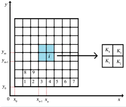
Since the fractional derivative is a non-local operator, the implementation of finite element method for fractional differential equations is very complex. The main problem is how to obtain the stiffness matrix. In [28], Roop investigated the computational aspects of the Galerkin approximating using continuous piecewise polynomial basis functions on a regular triangulation of the domain. In this section we give the computational details, in which the bilinear functions are chosen as the basis functions. The computational domain is Ω =

[ ] [ ]

a b, × c d, and the number of computational grid is N₁×N₂.

First of all, we consider the problem of finding the fractional derivative of each of the basis function 2

aDx i

(13)

[image:13.595.207.419.84.264.2]

Figure 1. Sketch for the element and node number.

1

2

3

4

1 1

0 0

1

1 2

2 2

0 0

2

1 2

3 3

0 0

3

1 2

4 4

0 0

4

1 2

1

1 1

4 1

1 1

4 1

1 1

4 1

1 1

4

i K

x x y y

l l

x x y y

l l

x x y y

l l

x x y y

l l

ψ ϕ

 −  − 

= = _ + _ + _

  

 −  − 

= =  −  + 

  

 −  − 

= = _ − _ − _

  

 −  − 

= =  +  − 

  

where

(

1 1

) (

2 2

) (

3 3

) (

4 4

)

0, 0 , 0, 0 , 0, 0 , 0, 0

x y x y x y x y are the centers of the blocks K K K K₁, ₂, ₃, ₄, and 1 1

2

n n

x x

l = − − ,

1 2

2

m m

y y

l = − − . Assume the coordinate of the ith node (seeFigure 1) is

(

xn,ym

)

, then we can derive

(

1

)

1

mod 1 , 1.

1

i n

n i N m

N

−

= − = +

− (41) If

(

x y,

)

∈K₁, we have

(

)

(

)

(

) (

)

1

1 2

2 2 0

1

1 2

1

1 2 ₀

1

1 2

1

1 d

4 1 2

1

4 2 2

n

x a x i a x _x

n

y y

D D x

l l

y y

x x

l l

α

α α

α

ψ ϕ ξ ξ

α

−

− −

 − 

= = − _ + _

Γ − _ _

 − 

= − _ + _

Γ − _ _

∫

If

(

x y,

)

∈K₂, taking notice that 1 2

0 0

y =y , we can get

(

)

(

)

(

) (

)

(

)

(

)

(

)

1 ₁

1 2

2 2 2 0

1 2

2

2 ₀

1 2

1

1 2 1 2

0

1

1 2

1

1 d

4 1 2

1

1 d

4 1 2

1

1 2

4 2 2

n

n n n _n

n

x a x i x x x x _x

x x

n n

y y

D D D x

l l

y y

x

l l

y y

x x x x

l l

α

α α α

α

α α

ψ ϕ ϕ ξ ξ

α

ξ ξ

α

− ₋

−

− −

−

 − 

= + = − _ + _

Γ − _ _

 − 

− − _ + _

Γ − _ _

 − _ _

= _{Γ −}  + _{ } − − − _

 