ARABIC NAMED ENTITY RECOGNITION IN CRIME DOCUMENTS

(1)

ISSN: 1992-8645 www.jatit.org E-ISSN: 1817-3195

125

SHORT-TERM TRAFFIC FLOW PREDICTION BY A

SUGENO FUZZY SYSTEM BASED ON GAUSSIAN

MIXTURE MODELS

1_{YANG WANG,} 2_{YANYAN CHEN}

1

Lecturer, Beijing Key Lab of Traffic Engineering, Beijing University of Technology, Beijing

2_{Prof., Beijing Key Lab of Traffic Engineering, Beijing University of Technology, Beijing}

E-mail: [email protected], [email protected]

ABSTRACT

The short-term traffic flow prediction is of great importance for traffic control and guidance. This paper presents an approach using a Sugeno fuzzy inference system whose input space is participated by a Gaussian mixture model and parameters are estimated by the least square estimation method. The proposed approach was evaluated on a benchmark problem of the Mackey-Glass time series and the collected traffic flow data via a comparison made with one of well-known methods. The experimental results indicate the proposed method is effective and competent.

Keywords: Short-term Prediction; Traffic Flow; Fuzzy Inference System (FIS); Gaussian Mixture Model

(GMM); Expectation Maximization (EM)

1. INTRODUCTION

In intelligent transportation systems (ITS), not only real time data of traffic flow is of great importance for traffic control and guidance, but also live and accurate traffic flow prediction can help to reduce unexpected malfunction in transportation. However, the road traffic system is a complex, open, and time-variant system which often exhibits highly randomness and uncertainty. This may well explain why accurate long-term prediction is not achievable and therefore much research efforts have been devoted to the short-term prediction (usually 2 to 15 minutes ahead). One primary methodology of the short-term traffic flow prediction is that the future state of the traffic system can be inferred from its previous states based on their correlation.

In literature, a wide spectrum of modeling methods has been adopted for the short-term traffic flow prediction, such as artificial neural network [1-2], regression model [3-4], Bayesian network [5], fuzzy logic system [6], and hybrid approach [7-8] etc.

Whenever the field knowledge is not available or incomplete to construct a model, the fuzzy inference system (FIS) is commonly one of the popular choices in that it is tolerant to noise, resistant to uncertainty, interpretable, easy to incorporate expert and field knowledge [9]. Two

types of FIS, namely Mamdani FIS [10] and Sugeno FIS [11] are widely accepted and applied to solve many real-world problems. Sugeno FIS is similar to Mamdani FIS in many aspects, but the output membership functions of Sugeno FIS are either linear or constant. As Sugeno FIS simplifies the defuzzification process, it is often adopted for the application that has a tight time constraint.

To construct a Sugeno-type fuzzy predictor mainly involves structure identification and parameter estimation, after determining the inputs. The clustering analysis is of great advantage as it not only defines the rules but also estimates the membership function parameters for the inputs

simultaneously. The clustering techniques

commonly used to build a Sugeno FIS are fuzzy c-means [12] and subtractive clustering methods [13]. After obtaining the rules from clustering results, the output from a typical Sugeno FIS is a weighted average of the output of each rule. And, the weights are normally estimated using the least square estimation technique [14].

(2)

126 estimation method. The next section is devoted to the detailed description of the algorithm developed to construct the fuzzy predictor. Following that, evaluation is presented before the paper is concluded.

2. CONSTRUCTION OF SUGENO FUZZY

PREDICTOR

2.1 Rule Base Identification

To create a Sugeno FIS, a Gaussian mixture model is firstly constructed by applying the Expectation Maximization (EM) algorithm to a set of the d-dimensional training data x = (x1, x2, …, xN) and then the mixture model is used to determine the rule base.

A mixture of K component Gaussians can be expressed as follow:

( )

(

)

(

)

∑

= − =     − − − π = ⋅ = K k k k T k k d k K k k k k w , ; f w f 1 1 1 2 1 exp ) 2 ( ) ( v x v x v x x Σ Σ Σ (1)

where f(x; vk, Σk) is the probability density function of kth component Gaussian with mean vector vk and covariance matrix Σk , and its weight wk satisfies

1

=

∑

= K k k

w

and

∀

i

:

w

_k

≥

0

(2)

To determine the parameter vector θ_{(i.e., w}_k_{, v}_k_,

and Σk for each component) for a Gaussian mixture model by EM, an unobserved latent variable y is added and this latent variable determines the component from which the observed data x originates. Thus, the log-likelihood function can be formulated as follow:

(

)

∑

(

)

= = N i i i f , ; L 1 ; , ln

ln θ _x _y _x _y θ (3)

The EM algorithm fits a mixture model to a set of training data by alternately performing between Expectation step and Maximization step.

Suppose the current step is at t step.

Expectation step: Firstly, the conditional

distribution of y given x under the current estimate of the parameters θ(t)_{is determined by Bayes}

theorem; ( )

(

)

(

( )

)

( )

(

)

∑

=

_K k t i i t i i t i i

|

,

k

f

|

,

k

f

,

|

k

f

1

θ

x

y

θ

x

y

θ

x

y

( )

(

)

(

)

( )

(

)

(

)

∑

= − −     − − − π    ₋ ₋ ₋ π = _K k k i k T k i k d t k k i k T k i k d t k w w 1 1 1 2 1 exp 2 2 1 exp 2 v x v x v x v x Σ Σ Σ Σ (4)

Then, the expectation of the log-likelihood function can be calculated as follow:

( )

(

θ

|

θ

)

E

_y_xθ( )

ln

f

(

x

,

y

|

θ

)

Q

t , | t

=

( )

(

)

(

)

∑ ∑

= = = = K k N i i i t i

i k| , ln f , |

f 1 1 θ y x θ x y (5)

Maximization step: Update the parameters that maximize the expectation of the log-likelihood function obtained in Expectation step.

( )t

(

( )t

)

Q

θ

|

max

arg

1

=

+ (6)

wk, vk, and Σk for next step (i.e., t+1 step) is derived as follow:

( ) ( )

(

)

( )

(

)

∑ ∑

∑

= = = +

=

N i K k t i i N i t i i t k

k

f

k

f

w

1 1 1 1

,

|

,

|

θ

x

y

θ

x

y

(7) ( ) ( )

(

)

( )

(

)

∑

= = +

=

_N i t i i N i i t i i t k

k

f

k

f

1 1 1

,

|

,

|

θ

x

y

x

θ

x

y

v

(8) ( ) ( )

(

)

(

( )

)

(

( )

)

( )

(

)

∑

= = + + + = − − = = N i t i i N i T t k i t k i t i i t k k f k f 1 1 1 1 1 , | , | θ x y v x v x θ x y Σ (9)

(3)

127

2.2 Parameter Estimation

As Gaussian membership function is adopted for the premises of FIS, the clustering results can be directly used to determine the parameters for the membership functions. To obtain a weight for each rule, we use a well-known method, least square estimation [14].

3. EXPERIMENTS

To evaluate the proposed approach (GMM-FIS for short), a benchmark problem, the Mackey-Glass time series, and a time series recorded for the traffic flow of a road in Beijing on November 1, 2006, were used and a well known approach, here called FCM-FIS [13], was selected for comparison purpose. The performances of FCM-FIS and GMM-FIS at training and prediction stages were examined based on the statistical criteria, Mean Absolute Percentage Error (MAPE) [6] and Normalized Root Mean Square Error (NRMSE) [15], as expressed in Equation 10 and 11. While MAPE can give us an idea about the averaged absolute relative error, NRMSE is able to identify which one is better when comparison is involved.

%

100 )

(

)

(

)

(

1 MAPE

1

×

−

=

∑

=

N

i

y

i

y

i

y

~

N

(10)

2 1

2

))

(

)

(

1 NRMSE

σ

i

y

i

y

~

N

i

∑

=

−

=

(11)

where

y

(i

)

and

~

y

(i

)

indicate the ith true and estimated vales of N length time series respectively, and

σ

is the standard deviation of the true values.

In order to make a fair comparison, two prediction algorithms were performed with as same parameter settings as possible. Due to the random initialization for the two prediction approaches (i.e., the initial centers generated randomly by the FCM and GMM algorithms), each experiment was independently conducted for 100 times and the averaged mean values are reported in this section.

3.1 Mackey-Glass Time Series Prediction

The Mackey-Glass time series is commonly used as a benchmark to test model identification and prediction, as it exhibits chaotic characteristics when the time-delay

τ

_{is large enough (e.g.}

τ

_is

17 in our test) [14]. In the experiments presented in this sub-section, the first 500 data of the Mackey-Glass time series was selected as the training set

and the last 500 data as the testing data. Each data point in the training set consists of

6)} ( ), ( 6), -( 12), -( 18), -(

{ +

= x t x t xt x t x t

x (12)

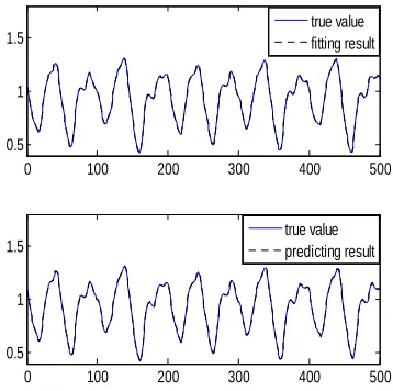
where the input space is constructed by the first four components and the last component forms the output. Fig. 1 and Fig. 2 show the results obtained by the two approaches (FCM-FIS and GMM-FIS) against to the actual Mackey-Glass time series during training and predicting stages, respectively. Note that the results typically generated for one run are illustrated in Fig. 1 and Fig. 2.

0 100 200 300 400 500

0.5 1

1.5 true value_{fitting result}

0 100 200 300 400 500

0.5 1

[image:3.612.332.511.253.431.2]

1.5 true value_{predicting result}

Fig. 1 Prediction Of The Mackey-Glass Time Series By FCM-FIS And The Solid And Dashed Lines Indicate The True And Estimated Values Respectively (The Upper For

Training And The Lower For Prediction)

From Fig. 1 and Fig. 2, it is evident that the values estimated by the two test algorithms are nearly identical to the true values of the Mackey-Glass time series, for both training and prediction. The invisible differences shown in Fig. 1 and Fig. 2 disclose litter information to us, the statistical results for the performances of the two algorithms over 100 independent runs are presented in Table 1 in a quantitative way.

It can be found from Table 1 that the MAPEs and NRMSEs for prediction are slightly smaller than those for training, implying adequate training samples have been supplied for the model

identification. Furthermore, the marginal

(4)

128

0 100 200 300 400 500

0.5 1 1.5

true value fitting result

0 100 200 300 400 500

0.5 1 1.5

true value predicting result

Fig. 2 Prediction Of The Mackey-Glass Time Series By GMM-FIS And The Solid And Dashed Lines Indicate The True And Estimated Values Respectively (The Upper For

[image:4.612.97.289.76.278.2]

Table 1. Comparison Of The Prediction Performance Using Mackey-Glass Time Series (Mapes And Nrmses

Were Averaged For 100 Times).

Criteria Algorithms Training Prediction

MAPE (100%)

FCM-FIS 0.5470 0.5342

GMM-FIS 0.5319 0.5188

NRMSE FCM-FIS 0.0303 0.0300

GMM-FIS 0.0278 0.0273

3.2 Traffic flow prediction

The prediction algorithm presented in this paper was further evaluated by using the traffic flow data collected and aggregated at intervals of 2 minutes duration for a road in Beijing on November 1st, 2006.

To eliminate the impact of the embedded noise, a de-noising process based on wavelet transform [16][17] was firstly performed by following the general procedures: 1) decomposition: compute the wavelet decomposition of the noisy data by applying a wavelet (‘db3’ in our case) to it at the specified level (2 decomposition levels); 2) detail

coefficients thresholding: select appropriate

threshold for each level and apply thresholding method (soft thresholding in our implementation) to remove the noises; 3) reconstruction: inverse wavelet transform of the threshold wavelet coefficients to generate clean data.

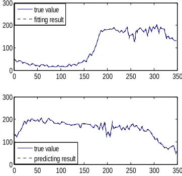
By using the first 350 data, the Sugeno FISs were constructed by the two algorithms with same settings, 2 inputs and 2 clusters. One-step-ahead

prediction was evaluated for the 350 data just beyond the first 350 data. Fig. 3 and Fig. 4 show the trained and predicted results by the two approaches against to the de-noised data.

0 50 100 150 200 250 300 350

0 100 200 300

0 50 100 150 200 250 300 350

0 100 200 300

Fig. 3 Prediction Of The Mackey-Glass Time Series By FCM-FIS And The Solid And Dashed Lines Indicate The True And Estimated Values Respectively (The Upper For

0 50 100 150 200 250 300 350

0 100 200 300

0 50 100 150 200 250 300 350

0 100 200 300

[image:4.612.328.510.156.333.2]

Fig. 4 Prediction Of The Mackey-Glass Time Series By GMM-FIS And The Solid And Dashed Lines Indicate The True And Estimated Values Respectively (The Upper For

[image:4.612.330.511.409.584.2]

(5)

129

Table 2. Comparison Of The Prediction Performance Using The Traffic Flow Collected For A Road In Beijing

On November 1st, 2006 (Mapes And Nrmses Were Averaged For 100 Times).

Criteria Algorithms Training Prediction

MAPE (100%)

FCM-FIS 2.3572 1.4541

GMM-FIS 2.3762 1.4751

NRMSE FCM-FIS 0.0392 0.0451

GMM-FIS 0.0395 0.0453

In Table 2, the MAPE values generated during the prediction stage are smaller than those during the training stages for both algorithms, but a revised case holds for NRMSEs. This may be caused by the relatively smaller true values for prediction than those for training, when calculating MAPE according to Equation 10. Nevertheless, the differences between training and prediction are inconsiderable, indicating the two algorithms performed reasonably well in terms of model generalization. As compared to those for training, a slightly higher NRMSEs obtained by the two algorithms for prediction implies that the over fitting problem is not significant. Finally, the negligible differences of MAPEs and NRMSEs obtained by FCM-FIS and GMM-FIS indicate that our approach is effective and competent.

4. CONCLUSIONS

This paper presented a prediction method based on a Sugeno FIS constructed by a Gaussian mixture model and the least square estimation technique. The evaluation was performed using the Mackey-Glass time series and the traffic flow recorded. The prediction results obtained by the two algorithms were compared. As compared to the well-known method used in this paper, the comparison results indicate that the prediction approach proposed in this paper is effective and competent. Finally, the authors gratefully acknowledge the financial support provided by Scientific Research Common Program of Beijing Municipal Commission of Education (KM201010005021) and the Scientific Research Foundation for the Returned Overseas Chinese Scholars, State Education Ministry (32004011201201).

REFRENCES:

[1] Y.S. Gu, Y.C. Li, J.C. Xu, and Y.P. Liu, “Novel Model based on Wavelet Transform and GA-Fuzzy Neural Network Applied to Short Time

Traffic Flow Prediction”, Information

Technology Journal, Vol. 10, No. 11, 2011, pp.

2105-2111.

[2] C.M. Zhu, C.P. Yan, X.L. Xu, and G.X. Wu, “Research on the Application of the Prediction of the Expressway Traffic Flow based on the Neural Network with Genetic Algorithm”,

Advanced Materials Research, Vol. 189, 2011,

pp. 4400-4.

[3] N. Zhang, Y.L. Zhang, and H.T. Lu, “Seasonal Autoregressive Integrated Moving Average and Support Vector Machine Models: Prediction of

Short-term Traffic Flow on Freeways”,

Transportation Research Record, Vol. 2215,

2011, pp. 85-92.

[4] J. Rice and E. van Zwet, “A Simple and Effective Method for Predicting Travel Times on Freeways”, IEEE Transactions on Intelligent

Transportation Systems, Vol. 5, No. 3, 2004, pp.

200-207.

[5] E. Castillo, J.M. Menendez, and S. Sanchez-Cambronero, “Predicting Traffic Flow using Bayesian Networks”, Transportation Research

Part B: Methodological, Vol. 42, No. 5, 2008,

pp. 482-509.

[6] Y.L. Zhang and Z.R. Ye, “Short-Term Traffic Flow Forecasting Using Fuzzy Logic System Methods”, Journal of Intelligent Transportation

Systems, Vol. 12, No. 3, 2008, pp. 102-112.

[7] M.C. Tan, S.C. Wong, J.M. Xu, Z.R. Guan, and P. Zhang, “An Aggregation Approach to

Short-term Traffic Flow Prediction”, IEEE

Transactions on Intelligent Transportation Systems, Vol. 10, No.1, 2009, pp. 60-69.

[8] C. Quek, M. Pasquier, and B.B.S. Lim, “POP-TRAFFIC: A Novel Fuzzy Neural Approach to Road Traffic Analysis and Prediction”, IEEE

Transactions on Intelligent Transportation Systems, Vol. 7, No. 2, 2006, pp. 133-146.

[9] Y. Wang, P. Beullens, H.H. Liu, D.J. Brown, T. Thornton, and R. Proud, “A Practical Intelligent Navigation System based on Travel Speed Prediction”, Proceedings of 11th International

IEEE Conference on Intelligent Transportation Systems, Beijing (China), October 12-15, 2008,

pp. 470-475.

[10] E.H. Mamdani and S. Assilian, “An Experiment in Linguistic Synthesis with a Fuzzy Logic Controller”, International Journal of

Man-Machine Studies, Vol. 7, No. 1, 1975, pp. 1-15.

[11] M. Sugeno, Industrial Applications of Fuzzy

Control, Elsevier, New York, 1985

(6)

130 Techniques for Fuzzy Model Identification”,

Fuzzy Sets and Systems, Vol. 106, No. 2, 1999,

pp. 179-188.

[13] P. Angelov, “An Approach for Fuzzy Rule-base

Adaptation using On-line Clustering”,

International Journal of Approximate Reasoning, Vol. 35, No. 3, 2004, pp. 275-289.

[14] G. Tsekouras, H. Sarimveis, E. Kavakli, and G.

Bafas, “A Hierarchical Fuzzy-clustering

Approach to Fuzzy Modeling”, Fuzzy Sets and

Systems, Vol. 150, No. 2, 2005, pp. 245-66.

[15] B. Hartmann, O. Banfer, O. Nelles, A. Sodja, L. Teslic, and I. Skrjanc, “Supervised Hierarchical Clustering in Fuzzy Model Identification”,

IEEE Transactions on Fuzzy Systems, Vol. 19,

No. 6, 2011, pp. 1163-76.

[16] M. Misiti, Y. Misiti, G. Oppenheim, and J.M. Poggi, Wavelets and their Applications, ISTE Publishing Knowledge, Hermes Lavoisier, 2007.

[17] D.L. Donoho, “De-Noising by

Soft-thresholding”, IEEE Transactions on

Information Theory, Vol. 41, No. 3, 1995, pp.