ISSN: 1992-8645 www.jatit.org E-ISSN: 1817-3195
MOTION TRAJECTORY PLANNING METHOD OF LANE
CHANGE FOR INTELLIGENT VEHICLE
1AIJUAN LI, 1SHUNMING LI, 1HUAN SHEN, 1XIAODONG MIAO, 2XIAO LI 1Energy and Power Engineering College, Nanjing University of Aeronautics and Astronautics, China
2
Department of Computer Engineering, Shandong College of Information Technology, China
ABSTRACT
The motion planning method of lane change for intelligent vehicle is an important component in the autonomous vehicle field. In order to make the intelligent vehicle drive on the urban environmental road smoothly when there is a barrier in the front, a new curvature-continuous obstacle avoidance trajectory planning method was introduced. The trajectory planning method based B-spline curves and the convex hull property of the B-spline curves is used. The effection of several nonholonomic constrained conditions is considered in this method. The nonholonomic constraints include obstacle avoidance constraint, curvature constraint, rotational speed constraint, speed constraint, state constraint and so on. The intelligent vehicle’s lane change reference trajectory is generated, the trajectory is collision-free and the curvature is continuous. The intelligent vehicle’s lane change simulation experiment was done to test the trajectory planning method. The result showed that the feasible trajectory can be generated by use of this article’s method. The curvature of the trajectory is continuous and every nonholonomic constraint condition was met.
Keywords: Intelligent Vehicle, Motion Trajectory Planning, Continuous Curvature, Lane Change, Β-spline
Curve
1
INTRODUCTIONThe intelligent vehicle is an important component of intelligent transportation system, the study of intelligent vehicle is becoming more and more important[1,2]. The dynamic trajectory planning technology is the precondition of the vehicle’s automatic control technology. The lane change motion trajectory planning technology of the vehicle is a key technology[3,4].
Many trajectory planning techniques for autonomous vehicles have been discussed in the literature. Among them, much of work on search algorithms provide computationally efficient way in discrete state spaces[5,6]. However, the resulting trajectories by such algorithms do not tend to be smooth and hence do not satisfy kinematic feasibility of the vehicle. Dubins trajectory is one of the most well-known methods to generate a smooth trajectory[7]. The trajectory has a drawback of discontinuity of curvature at the joint nodes connecting the lines and arcs. Tracking such trajectory requires a vehicle to stop and reposition in order to alter its steering angle. So curvature continuity is an important requirement for trajectory guidance applications. B-spline curve’s curvature is continuous and some trajectory planning techniques have been discussed based on B-spline curves[8,9].
Our trajectory planning algorithm is based on the B-spline curves and the convex hull property of the B-spline curves is used. The algorithm imposes obstacle avoidance constraint, curvature constraint, rotational speed constraint, speed constraint, state constraint such that the trajectory is curvature-continuous and the vehicle can track the planned trajectory collision-freely.
2
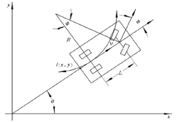
THE VEHICLE MODELThe simplified model of the autonomous vehicle can be expressed in the Fig. 1. Where idefines the
[image:1.612.322.513.600.722.2]position of the rear axle’s midpoint in an Euclidean reference frame. The vehicle’s front wheel is steering wheel and the rear wheel is driving wheel. The kinematics of a vehicle having axle base L can be described by a kinematic model satisfying as Eq. 1:
ISSN: 1992-8645 www.jatit.org E-ISSN: 1817-3195
cos 0
sin 0
0
0 1
x y
v k
k
θ θ
σ θ
= +
(1)
Where:
2
(1 ) tan , cos
k= L ϕ σ = =k ω L ϕ (2) Where θ means the orientation of the vehicle
relative to the x-axis and φ is the front wheel’s steering angle, R is the vehicle’s curvature radius, the inputs v and ω are the vehicle’s linear velocity at the point i and the steering angular velocity, respectively. The state vector is
q
=
[
x
,
y
,
θ
,
k
]
T. Furthermore, thecurvature and the curvature changerate are restricted according to:
max max
max max 2 max
1 tan
1 1
cos
k k
L
L L
ϕ
σ σ ω ω
ϕ
≤ =
≤ = ≤
(3)
3
MAKE SURE OF THE STARTINGPOSITION
The parameters of lane change driving when the vehicle running on the urban environmental road is shown as Fig. 2.
Fig.2 The Parameters Of Lane Change Driving
The lane change driving is mainly decided by three parameters: the parallel distance D between the starting and the ending positions, the arc of circumference A2 of radius R2 and the arc of
circumference A1 of radius R1. The relationship
equations is as follows:
(
)
(
)
1 2
1 2
sin 0
(1 cos )
R R D
R R y
θ θ
+ − =
+ − = ∆ (4)
Where θ and Δy are defined in Fig. 2, H is the lateral distance between the obstacle and the road side. Each value of the parameters [R1, R2, D] can determines a lane change driving.
The trajectory is a collision-free trajectory if the following condition is satisfied:
1 1max 2 [ 2 min, 2max]
R <R R ∈ R R (5)
2 2 2
1max
2 2 2
2 min
2 max 1
max 2
( )
2( )
1 cos
x y
y
C C L
R
P
d L H y
R
H y d
y
R R
θ
+ −
=
+ − − ∆
=
− ∆ − ∆
= −
−
(6)
Where d is the wide of the vehicle, L is the wheelbase, θmax is the maximum value of θ when the
trajectory is tangent to the point (Cx, Cy) and R1, R2> Rmin.
When R1=Rmin and R2=R2min, the distance D of
the collision-free trajectory is the minimum value:
(
)
2min 2 y min 2min y
D = ∆ R +R − ∆ (7)
When R1= Rmin and R2= R2max, the distance D of
the collision-free trajectory is the maximum value:
(
)
2max 2 y min 2max y
D = ∆ R +R − ∆ (8)
4
THE TRJECTORY PLANNING METHOD BASED B-SPLINE CURVE4.1 B-Spline Curve
A B-spline curve is a parametric curve whose curvature is continuous even at the joints between adjacent segments. This type of curves is specified by a set of points called control vertices. Let the control polygon be composed of control vertices [V0, V1, . . . , Vm], the curve will be composed of
m−2 segments. Thus, the ith curve segment is determined by four control vertices Vi+r, r =-2, -1, 0,
1. The coordinates of the point Qi,4(u) on the ith
curve segment are: 1
1 2
2
( ) ( , , )
i r i r
r
Q u b β β u V+
=−
=
∑
(9)Where 0≤u<1; i = 2, 3, ..., the weighting factors
br are scalar functions evaluated at any value of the
domain parameter u and on each shape parameter β1
and β2.
Previous works have experimentally shown that cubic splines represent the best choice. In that case,
ISSN: 1992-8645 www.jatit.org E-ISSN: 1817-3195
2,4
1,4
2 0,4
3 1,4
1 1 1 1
6 2 2 6
1
( ) 2 1
0 1
( ) 3 2
( ) 1 1 1 1
6 2 2 2
( )
1
0 0 0
6
b u
u b u
b u u
b u u
−
−
− −
−
= ×
−
(10)
One of the most significant property of the
B-spline curves is the convex hull. If the control vertices are over an arc of circumference and the distance δ between them is regular, an important consequence can be derived[10]. Let the vertices of
a B-spline segment be over an arc of the
circumference C of radius R (see Fig. 3). If the
Fig.3 Sketch Of Control Vertices Over An Arc Of Circumference
distance between them is δ, where δ≤(π/6)R, then the
B-spline segment is out of the circle C’ , whose radius R’ is:
3 cos
2
R R
R
δ
′ <
(11)
It can be experimentally tested that the curvature radius of the segment is upper bounded by R and lower bounded by R’. Therefore, if the value of the curvature radius of the segment has to be kept between R and R’, then δ should satisfy:
2 a cos 3
R R
R
δ < ′
(12)
This constraint also assures that the segment will be between both arcs of circumference.
4.2 Selection Of Δs
4.2.1 Collision-free constraint
According to the Fig.2, only the curve’s curvature radius is between the arc of R2 and the arc of Rc, the
trajectory meet the collision-free condition. Rc is the
minimum radius avoiding the collision of the vehicle’s right front and right behind. The value of
Rc is as follows:
(
)
2(
)
2x x
c x y
R = C −O + C −O (13) Where (Ox, Oy) is the centre of the arc A2. We
can see from the Fig. 3 and Eq. 4 that:
x 1 2
y 2
( )sin
y
O D R R
O R
θ
= = +
= − ∆ (14)
Then, according to Eq. 12 the trajectory is collision-free if the following sufficient condition is satisfied:
c 2
1
2 2
a cos 3
s
R R
R
δ ≤δ <
(15)
Due to the fact that R2minis the lowest value of R2,
the trajectoryis collision-free if the curvature radius is over R2min, according to Eq. 12, we can get:
2 2min
2
2 2
a cos 3
s
R R
R
δ ≤δ <
(16)
4.2.2 Bounded curvature
The curve radius’ value of an admissible trajectory has to be over the minimum radius Rmin of
the vehicle: R1≥Rmin, R2≥Rmin. Then, according to
the previous section the trajectory should meet this condition:
1 min
3
1
2 min
4
2 2
a cos 3
2 a cos 3
s
s
R R
R
R R
R
δ δ
δ δ
≤ <
≤ <
(17)
4.2.3 Steering velocity constraint
Although B-spline curves are
curvature-continuous trajectory, the curvature’s change should be smooth enough for a successful trajectory tracking. It can be experimentally illustrated that changes for lane change running. The changes of curvature can be approximated by the linear relations as Fig. 4. The curvature change need to meet the Eq. 18.
ISSN: 1992-8645 www.jatit.org E-ISSN: 1817-3195 1 0 3 2 5 4 1 1 1 1 2 2 2 2 3 3 3 3 3 s s s s s s d m k ds d m k ds d m k ds ρ ρ δ ρ ρ ρ δ ρ ρ δ
< = ⋅
+
< = ⋅
< = ⋅
(18)
If v = ds/dt represents the vehicle linear velocity, the curvature change velocity will satisfy:
1 0 3 2 5 4 1 2 3 t t t t t t d m v dt d m v dt d m v dt ρ ρ ρ < < < (19)
Where [t0, t1], [t2, t3], [t4, t5] represent the period
of time when the curvature is changing. On the other hand, the curvature change velocity due to the steering system is:
2 L cos ϕ ρ ϕ = ⋅
(20)
Ifφmaxis the maximum angular velocity of the steering system, only the curvature velocity change meets Eq. 21 along the curve, the steering mechanism could properly follow the curve.
max
3 m
k v
L
ρ ρ ρ ϕ
δ
⋅ ⋅ = ≤ = (21)
We can gain that the value ofδs satisfies the following constraints:
(
)
1 1
5
max
1 1 2
6 max 2 2 7 max 3 3 3 s s s
k v L
k v L
k v L
ρ δ δ ϕ ρ ρ δ δ ϕ ρ δ δ ϕ ⋅ ⋅ ≥ = ⋅ + ⋅ ≥ = ⋅ ⋅ ≥ = (22)
Where k1=6.6, k2=3.2 and k3=6.6 have been
experimentally gained.
4.2.4 Make sure the value of δs
In order to generate B-spline curve, the value of
δs can be accomplished from (15), (16), (17), (22):
5 6 7 vel s col
1 2 3 4
max( , , )
min( , , , )
δ δ δ δ δ δ
δ δ δ δ
= ≤ ≤
= (23)
The value δvel is chosen for practical reasons. Further evaluation assures that this selection
accomplishes the constraint condition δs≤δcol . Considering that (δ1, δ2, δ3, δ4) are mainly related to
geometrical constraints, while (δ5, δ6, δ7) depend on
the vehicle velocity and the velocity of the steering system. It could be possible to have δvel> δcol, in this
case, δs=δcol. We can see from the Eq. 22 that if the
constraint condition is met then the initial velocity
vinihave to change. The velocity’s upper bound is:
(
)
L k v v L k v v L k v v s s s ⋅ ⋅ ⋅ ⋅ = ≤ ⋅ + ⋅ ⋅ ⋅ = ≤ ⋅ ⋅ ⋅ ⋅ = ≤ 2 3 max 3 2 1 2 max 2 1 1 max 1 3 3 3 ρ δ φ ρ ρ δ φ ρ δ φ (24)We choose the vmax =min
(
v v v1, 2, 3)
as the new velocity. But the value of the velocity can not lower than the minimum velocity vlow, if v is bellow thisvalue, the vehicle has to perform a discontinuous curvature trajectory.
4.3 The Generation Of The Vertices
In order to generate feasible trajectory, not only the starting and ending points should belong to the
B-spline curve, but also the curve has to be tangent to the vehicle orientation. Auxiliary vertices are created at each extreme in order to achieve such conditions. If the first vertex is V0 and ρs, ρs are
the first and the second derivative vector specifications, respectively. Then three phantom vertices are given by:
1 0 s s
2 0 s
3 0 s s
1 3 1 6 1 3 V V V V V V ρ ρ ρ ρ ρ − − − = + + = − = − + (25)
If Vmis the last vertex, three more vertices are
defined: Vm+1, Vm+2 and Vm+3. The values are
determined by an equation similar to Eq. 25. In this paper the value ρs=0 has been used.
The trajectory planning problem is changed to the selection of δs. The value of δs is ensured through
ISSN: 1992-8645 www.jatit.org E-ISSN: 1817-3195
5
SIMULATION EXPERIMENTAL RESULTSAccording to the urban environmental road environment, the vehicle lane change driving simulation experiment was done to test this article’s method. A certain type of vehicle’s length and width is 4.199 m and 1.786 m, respectively, the axle base is 2.578 m., the maximum curvature is ρmax=0.165 m-1,
the maximum angle velocity isφmax=0.4 rad/s, the
initial velocity is vini=8 m/s, the minimum velocity is vlow=6 m/s. By means of using the trajectory
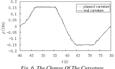
[image:5.612.97.294.271.406.2]planning method, the simulation experiment results of the vehicle lane change driving are shown in Fig. 5 and Fig. 6. Fig. 5 is
Fig.5 The Result Of The Vehicle Lane Change Driving Using This article’s method
Fig. 6 The Change Of The Curvature
theresult of the vehicle lane change driving using this article’s method. Fig. 6 is the change of the curvature.
In Fig.5 and Fig.6, a curvature-continuous reference trajectory is generated and the vehicle can follow the planned trajectory smoothly within the constraints. In this experiment, δcol=0.65 m and δvel=0.87 m. According to Section 4.2.4, the value of δs was chosen as δs=δcol=0.65 m. As a consequence
of not reducing the velocity, the steering system cannot follow appropriately the curvature change. Notice that a feasible driving would be obtained with
vmax=7.7 m/s, vmax>vlow. The maximum angle
velocity is φ=0.36 rad/s in this experiment, φ=0.36 rad/s<φmax=0.4 rad/s. Therefore, the driving was
successfully executed.
We can see from the experiment that the vehicle can follow the trajectory smoothly and collision-freely by using this article’s method.
6
CONCLUSIONSIn this paper a method of lane change for intelligent vehicle to generate curvature-continuous trajectory has been presented. The conclusions can be summarized as follows:
(1) The planned trajectory is
curvature-continuous by using the method. This property can ensure the vehicle to follow the planned trajectory smoothly.
(2) Several constraint conditions have been considered to assure the existence of collision-free admissible trajectory in the method. The vehicle can track the trajectory accurately.
(3) The simulation experiment results showed that this article’s method is reasonable and feasible. The vehicle can follow the trajectory smoothly and collision-freely.
REFRENCES:
[1] Β. Muller, J. Deutscher, S. Grodde, “Continuous Curvature Trajectory Design and Feedforward Control for Parking a Car”, IEEE Transactions on Control Systems Technology, Vol. 15, No. 3, 2007, pp. 541-553.
[2] H. Gharavi, K. V. Prasad, P. Ioannou, “Scanning Advanced Automobile Technology”, Proceedings of the IEEE, Vol. 95, No. 2, 2007, pp. 328-333.
[3] D. B. Ren, J. Y. Zhang, J. M. Zhang, et al, “Trajectory planning and yaw rate tracking control for lane changing of intelligent vehicle on curved road”, Science China (Technological Sciences), Vol. 54, No. 3, 2011, pp. 630-642. [4] G. Sébastien, V. Benoit, M. Saïd, et al,
“Maneuver-Based Trajectory Planning for Highly Autonomous Vehicles on Real Road with
Traffic and Driver Interaction”, IEEE
Transactions on Intelligent Transportation System, Vol. 11, No. 3, 2010, pp. 589-606. [5] A. Nash, K. Daniel, S. Koenig, et al, “Theta*:
Any-angle path planning on grids”, Proceedings of the IEEE, Vol. 95, No. 2, 2007, pp. 328-333. [6] L. Podsedkowski, J. Nowakowski, M. Idzikowski,
[image:5.612.99.288.399.513.2]ISSN: 1992-8645 www.jatit.org E-ISSN: 1817-3195
[7] F. Lamiraux. and J. -P. Laumond, “Smooth motion planning for car-like vehicles”, IEEE Transactions on Robotics and Automation, vol. 17, No. 4, 2001, pp. 498-502.
[8] Y. Liu, Y. L. Ma and T. Li, “Parallel Parking Path Generation Based on Bezier Curve Fitting”, Science & Technology Review, vol. 29, No. 11, 2011, pp. 59-61.