HIGH-DIMENSIONAL HIERARCHICAL OLAP : A PREFIX–
INDEX HIERARCHICAL CUBING APPROACH
1KONGFA HU, 2ZHE SHENG, 3LING CHEN
1 Prof., Department of Computer Science and Engineering, Yangzhou University, 225009,China 2 Master , Department of Computer Science and Engineering, Yangzhou University, 225009,China
3 Prof., Department of Computer Science and Engineering, Yangzhou University, 225009,China
E-mail: [email protected]
ABSTRACT
The pre-computation of data cubes is critical for improving the response time of OLAP(online analytical processing) systems and accelerating data mining tasks in large data warehouses. However, as the sizes of data warehouses grow, the time it takes to perform this pre-computation becomes a significant performance bottleneck. In a high dimensional OLAP, it might not be practical to build all these cuboids and their indices. In this paper, we propose a multi-dimensional hierarchical cubing algorithm, Prefix-index hierarchical cubing, based on an extension of the previous minimal cubing approach. This method partitions the high dimensional data cube into low dimensional cube segments. Such an approach permits a significant reduction of CPU and I/O overhead. Experimental results show that the proposed method is significantly more efficient than other existing cubing methods.
Keywords: Data cube, High dimensional OLAP, Prefix-Indexing cubing
1. INTRODUCTION
OLAP refers to the technologies that allow users to efficiently retrieve data from the data warehouse for decision support purposes [1]. A lot of research has been done in order to improve the OLAP query performance and to provide fast response times for queries on large data warehouses. A key issue to speed up the OLAP query processing is efficient indexing and materialization of data cubes [2,3,4]. Recently, many data cubing algorithms, such as BUC [5], H-cubing [6], quotient cubing [7], and star-cubing [8], have been proposed.
A key challenge for efficient data cubing is that, in large data warehouse applications, data usually has a high dimensionality (e.g. more than 100 dimensions) and each dimension has multiple hierarchy levels. Since data cube grows exponentially with the number of dimensions and number of hierarchy levels, it is generally too costly in both computation time and storage space to materialize a full high-dimensional data cube.Although some new algorithms, such as condensed cube [9], dwarf cube[10], or star cubes [8], can delay the explosion, they do not solve the fundamental problem[11]. The minimal cubing approach by Li and Han [11] can alleviate this problem, but it does not consider the dimension hierarchies and cannot efficiently handle OLAP
queries. In this paper, we develop an efficient cubing algorithm that supports dimension hierarchies for high-dimensional data cubes and answers OLAP queries efficiently.
The proposed cubing algorithm has the following salient features. 1) It supports not only high-dimensional data cubes but also hierarchical data cubes with multiple levels in a dimension. 2) The decomposition of the data cube space leads to significant reduction of processing and I/O overhead for many queries by restricting the number of cube segments to be processed for both the fact table and bitmap indices. 3) The prefix bitmap index is designed to support efficient OLAP by allowing fast look-up of relevant tuples. 4) The proposed cubing algorithm supports parallel I/O, parallel processing, and load balancing among disks and processors.
2. SHELL CUBE SEGMENTATION
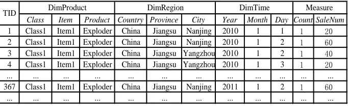
To illustrate the method ,a tiny warehouse, Table 1, is used as a running example.
For a cube of d dimensions, it will create 2d cuboids. If we consider the dimension hierarchies of each dimension, the cube will create
1
( 1)
d
i i
h
=
+
∏
cuboids (where hi is the number of hierarchy
Table 1 has three dimensions: DimProduct, DimRegion and DimTime. The DimProduct dimension has three hierarchies as (Class,Item,Product), the DimRegion dimension has three hierarchies as (Country,Province,City),and the DimTime dimension has three hierarchies as (Year,Month,Day). Therefore, this cube with three dimensions will generate in total
1
( 1) (3 1) (3 1) * (3 1) 64
d i i
h =
+ = + ∗ + + =
∏
cuboids suchas
[image:2.612.140.481.204.308.2]{(Product,City,Day),(Product,City,Month),(Product ,City,Year), (Product,City,All) ,..., (All,All,All)}. But in a high-dimensional warehouse, there is a substantial I/O overhead for accessing a fully materialized data cube.
Table 1. A Sample Warehouse
Class Item Product Country Province City Year Month Day Count SaleNum
1 Class1 Item1 Exploder China Jiangsu Nanjing 2010 1 1 1 20
2 Class1 Item1 Exploder China Jiangsu Nanjing 2010 1 2 1 60
3 Class1 Item1 Exploder China Jiangsu Yangzhou 2010 1 2 1 40
4 Class1 Item1 Exploder China Jiangsu Yangzhou 2010 1 3 1 20
... ... ... ... ... ... ... ... ... ... ... ...
367 Class1 Item1 Exploder China Jiangsu Nanjing 2011 1 2 1 60
... ... ... ... ... ... ... ... ... ... ... ...
Measure
TID DimProduct DimRegion DimTime
A partial solution which has been implemented in some commercial data warehouses is to compute a thin shell cube. For example, one might compute all the cuboids with 3 dimensions or less in a 30-dimension data cube. There are two disadvantages of this approach. First, it still needs to compute
1 30 2 30 3
30 C C
C + + = 4525 cuboids if there is no
hierarchies and it needs to compute
2h*(
1 30 2 30 3
30 C C
C + +
)=23*4525=36200 cuboids when each dimension has h=3 levels dimension hierarchies. Second, it does not support OLAP in a large portion of the high-dimensional cube space.
In this paper, we propose an orthogonal way to partition the cube space. We partition all the dimensions of a cube into subsets called the cube segments. For example, for a warehouse of 30 dimensions, D1, D2,...,D30, we first partition the 30
dimensions into 10 Cube segments of size 3: (D1,D2,D3), (D4,D5,D6),...,(D28,D29,D30). For each
cube segment, we compute its full data cube. For example, in Cube segment(D1,D2,D3),we compute
the eight cuboids:{(D1,D2,D3),(D1,D2,All),(D1,All,D3),(All,
D2,D3),
(D1,All,All),(All,D2,All),(All,All,D3),(All,All,All)}
. If we consider that each dimension of the 3-D cube (D1,D2,D3) has three hierarchy levels as
D1(L L L11, 12, 13),D2(L L L12, 22, 23), D3(L L L13, 32, 33), we will
compute 64 cuboids:{( 1 2 3 3, 3, 3
L L L ), ( L L L13, 23, 32 ) ,...,(All,All,All)}.
The benefit of this model can be seen by a simple calculation. For a cube of 30 dimensions without hierarchy, if we partition it into 10 segments, each with 3 dimensions, each segment will have 8
cuboids and there are only 8×10 = 80 cuboids to be computed. If each dimension has three hierarchy levels, then each segment will have 64 cuboids as shown above, and there are in total 64×10 = 640 cuboids to be computed. Comparing this to the 36200 cuboids needed by the shell cube technique, the savings in cubing time and space are significant.
Lemma 1. Given a warehouse of T tuples and d dimensions, the entire shell Cube segment will create
1
* /
f i f i
C d f
=
∑
=( 2f∗ d/ f ) cuboids and
needs O(T*
1
* /
f i f i
C d f
=
∑
)=O(T* ( 2f /d f
∗ ))
storage space, while the partial cube will create
∑
=
f
i i d
C
1 cuboids and needs O(T*
∑
=f
i i d C
1 ) storage
space, and the full cube will create 2d cuboids and needs O(|T|*2d) storage space.
Rational. In the shell Cube segment method, the cube partition into d/f cube segments. For each
cube segment will create 1
f
C
cuboids of1-dimension, 2
f
C cuboids of 2-dimension,..., f f
C cuboids of f-dimension and one cuboid(All,All, ...,All). Thus each cube segments will create
( 1 2
1 f
f f f
C +C + + C + ) =
1
f i f i
C
=
∑
cuboids. So the entire shell Cube segment will create1
* /
f i f i
C d f
=
∑
=( 2f ∗ d/ f) cuboids and needsO(T*
1
* /
f i f i
C d f
=
In partial cube, we select f dimensions from the d dimensions to create the partial cube . It will create
1
d
C
cuboids of 1-dimension, 2d
C cuboids of
2-dimension,...,
f d
C cuboids of f-dimension. Thus the f
partial cube will create
f d d
d C C
C1 + 2++
=∑= f i i d C 1
cuboids and needs O(T*∑=
f
i i d
C
1 ) storage space.
In full cube, for each dimension D, the dimension of its aggregate cuboids is D or All. For every dimension {D1,...,Dd}, the dimension of its
aggregate cuboids is chosen form the 2-values {Di,All}. So for the entire full cube, it will create
1 2
d
i=
∏
=2d cuboids and needs O(|T|*2d) storage space.Lemma 2. If we consider each dimension has h hierarchies, our prefix-index cubing method will create
1
( 1) * /
f
i i
h d f
=
+
∏
=( (h+1)f ∗ d/ f ) cuboids, while the minimal cubing method of Li’s and Han’s will create1 1 ( ) * / i i h f i j f h i j
C C d f
= =
∑ ∑
=( ( )
2 f+h *d/ f) cuboids.
Rational. In prefix-index cubing method, each dimension Di has hi hierarchies, the dimension
hierarchies of its aggregate cuboids is chosen form
the (hi+1)-values {
i h i i L L
L1, 2,, ,All}. So it will
create
1
( 1) * /
f
i i
h d f
=
+
∏
=( h
d f
f
/ ) 1
( + ∗ ) cuboids.
In the minimal cubing method, the cube partition
into
d/ f
cube segments. For each cube segmentswill create
∑
=f
i i f
C
1 cuboids for the f dimensions cube
segments. For each dimensions of these cube
segments have hi hierarchies and create
∑
= i i h j j h C 1dimensional hierarchy cuboids. So the entire
minimal cubing will create
1 1 ( ) * / i i h f i j f h i j
C C d f
= =
∑ ∑
=( ( )
2 f+h *d/ f) cuboids.
3. PREFIX BITMAP INDEXING
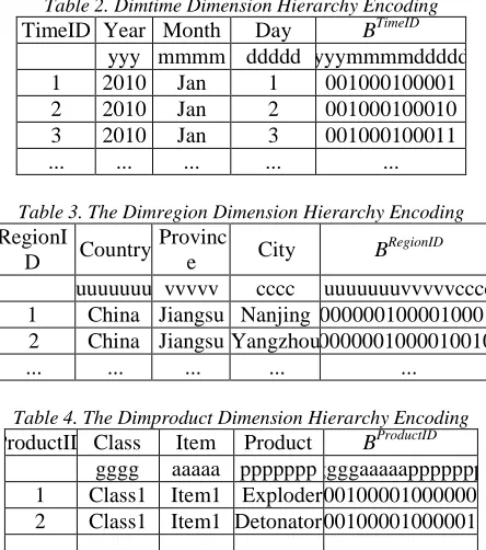
As we will see, our multi-dimensional fragmentation permits eliminating some bitmaps, thus improving storage and access overhead. We propose this novel hierarchical encoding on each
[image:3.612.311.533.183.434.2]dimension table. The encoding is implemented through the assignment of a special surrogate key on each dimension table tuple, called dimension hierarchical encoding.We can create the DimRegion,DimTime and DimProduct dimension hierarchy encoding shown in Table 2,Table3 and Table4.
Table 2. Dimtime Dimension Hierarchy Encoding TimeID Year Month Day BTimeID
yyy mmmm ddddd yyymmmmddddd
1 2010 Jan 1 001000100001
2 2010 Jan 2 001000100010
3 2010 Jan 3 001000100011
... ... ... ... ...
Table 3. The Dimregion Dimension Hierarchy Encoding RegionI
D Country Provinc
e City B
RegionID
uuuuuuu vvvvv cccc uuuuuuuvvvvvcccc 1 China Jiangsu Nanjing 0000001000010001 2 China Jiangsu Yangzhou 0000001000010010
... ... ... ... ...
Table 4. The Dimproduct Dimension Hierarchy Encoding ProductID Class Item Product BProductID
gggg aaaaa ppppppp ggggaaaaappppppp 1 Class1 Item1 Exploder 00100001000000 2 Class1 Item1 Detonator 00100001000001
... ... ... ... ...
Lemma 3. Our prefix-index cubing method needs O(T* (h+1)f ∗ d/ f)*log2m/8) storage space, while the minimal cubing method of Li’s and Han’s needs O(T*( ( )
2f h * /
d f
+
)*log10m ) storage space.
Rational. In prefix-index cubing method , the
member of each dimension needs
log2m
bitsdimension hierarchical encoding. So the storage space of prefix-index cubing method needs
O(T*( h
d f
f
/ ) 1
( + ∗ )*
log2m
/8) bytes. In theminimal cubing method , the member of each
dimension needs
log10m
integer indices. So thestorage space of the minimal cubing needs O(T*( ( )
2f+h *d/ f)log10m*) bytes.
To compute a data cube for this database with the measure avg() (obtained by sum()/count()), we need to have a tid-list for each cell: {tid1,..., tidn}. Because each tid is uniquely associated with a particular set of measure values, all future computations just need to fetch the measure values associated with the tuples in the list. In other words, by keeping an array of the ID-measures in memory for online processing, one can handle any complex measure computation.Table 8 shows what exactly should be kept, which is substantially smaller than the database itself.
Table 5. Dimproduct Dimension TID
BProductID TID List
0001000010000001 1-2-3-4-367
... ...
Table 6. Dimregion Dimension TID
BRegionID TID List
0000001000010001 1-2-367 0000001000010010 3-4
... ...
Table 7. Dimtime Dimension TID
BTimeID TID List
001000100001 1
001000100010 2-3
001000100011 4
... ...
Table 8. TID- Measure Array Of Table 2
tid Count SaleNum
1 1 20
2 1 60
3 1 40
4 1 20
... ... ...
4. PARALLEL HIERARCHICAL
AGGREGATION ALGORITHM
4.1 Parallel Construction of Shell Cube Segments
The data cube can be distributed across a set of parallel computers by parallel constructing the Cube segments. Therefore, for the end-user and other potential applications, we consider this data cube as one large virtual cube, which is distributed across a set of parallel computers, which manage the creation, updates and querying of the associated cube portions. To develop appropriate scheduling
mechanisms for these management tasks, we consider that the virtual cube is split into several smaller parts, called Cube segments. But a Cube segment could furthermore also be split into smaller segments and so on, till we achieve the level of chunks. They can then be assigned to parallel computers, having sequential or parallel computing power, which are responsible for their management. The algorithm for shell prefix cube segment parallel computation can be summarized as follows.
Algorithm 1 (Parallel computation of cube segments)
Input: A base cuboid BC of n dimensions:(D1; ...
;Dn).
Output: (1) A set of Cube segment partitions {P1;..., Pk} and their corresponding (local) Cube
segments {CS1; ... ; CSk}, where Pi represents
some set of dimension(s) and P1... Pk are all
the n dimensions, and (2) an ID measure array if the measure is not tuple-count such as {sum, avg}. { partition the set of dimensions :(D1; ... ;Dn) into a set
of k Cube segments {P1;..., Pk};
scan base cuboid BC once and do the following with parallel processing
{ insert each <tid, measure> into ID-measure array;
for each attribute value ai of each dimension Di
build an dimension hierarchy encoding index entry: <B: TID list>;}
parallel processing all segment partition Pi as
follows
build a local Cube segments CSi by intersecting
their corresponding tid-lists and computing their measures;}
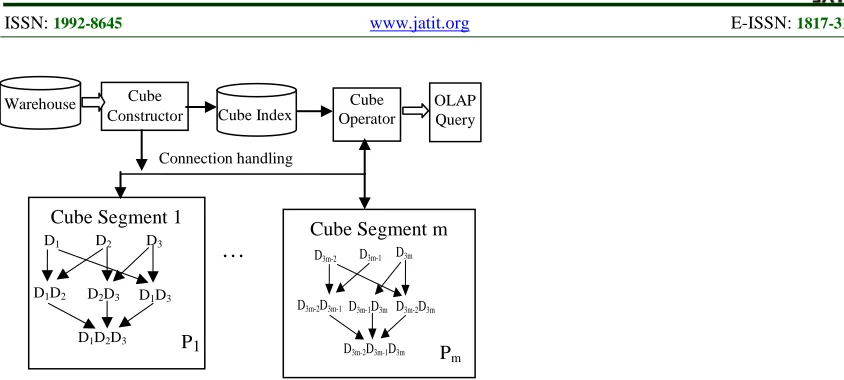
We can parallel construct the high dimensional cube with the Cube segments parallel construction. The system architecture of these shell Cube segment parallel construction is shown in Figure 1.
Fig. 1. The System Architecture of Parallel Construction of Shell Cube Segments
4.2 Efficient OLAP query handling
Based on the bitmap indexing, we can efficiently retrieve the matching hierarchy levels of each dimension, evaluate the set of query ranges for each dimension, and improve the efficiency of OLAP queries. A key property of our encoding is that it is a prefix indexing scheme that allows one to quickly retrieve a path prefix for each dimension.
The path prefix of the member i k
d
of the
hierarchy level i
j
L
is defined as
DMPrefixpath(DTree,
i k
d
)=
1
i j=
∪
DMPrefixpath(DTree,Parent( j k
d
))={
Ancestor( i k
d
)}, where Ancestor(d
ki ) is the allancestors of the member i k
d
according to its dimension hierarchy tree. The encoding prefix of
the member i k
d
is defined as Bprefix(B i k
d
, i m
L
−1)=
B i k
d
>>
∑
=j
m l (Bit
i l
L
), where m={1, ...,j}.
By using encoding prefix, we can register the dimension hierarchy encoding and its TID list for every dimension hierarchy for each dimension. For example, the dimension hierarchy encoding and its TID list associated with the dimension hierarchies
Month and Province are shown in Table 9, and so on.
For each fragment, we compute the complete data cube by intersecting the TID-lists in the dimension and its hierarchies in a bottom-up depths-first order in the cuboid lattice (as seen in [8]). For example, to compute the cell
{0001000010000001, 0000001000010001, 0010001}, we intersect the TID lists of BProductID
=0001000010000001, BRegionID
=0000001000010001, and Bprefix(BTimeID,Month)= 0010001 to get a new list of {1,2}. The algorithm of efficient OLAP query can be summarized as follows.
Table 9. Month hierarchy encoding Prefix AND its TID
BTimeID Bprefix(BTimeID,Month) TID List
001000100001 0010001 1-2-3-4
001000100010 001000100011
... ... ...
010000100001 0100001 367
... ... ...
Algorithm 2 (OLAP Query)
Input: A set of precomputed shell Cube Segments for partitions {P1,..., Pk}; an TID
measure array; and a OLAP query
Q<a1,...,an,M>.(The ai is attribute for the dimension
Ai and M is the measure of the query.)
Output: The computed measure
{ ascertain all Cube Segment CSi according as
the each dimension attribute of the query Q<a1,...,an,M>;
for each CSi
{ compare the CSi with query
Q<a1,...,an,M> using the Lattice and find
the all dimension Di of CSi∩{a1,...,an}
with parallel processing;
compute the TID List of the all BCi cells
of CSi∩{a1,...,an} in Di and its aggregate
Cuboids; Cube Segment 1
D1 D2 D3
D1D2 D2D3 D1D3
D1D2D3 P1
Cube Segment m
D3m-2 D3m-1 D3m
D3m-2D3m-1
D3m-2D3m-1D3m
D3m-1D3m D3m-2D3m
Pm
Warehouse Cube
Constructor Cube Index
Cube Operator
OLAP Query
Connection handling
intersect the TID List of th BCi and
compute the query result set RQ{TID List};
compute the aggregate with each TID of the TID-measure array from the set RQ{TID List};}}
This method uses the small dimension hierarchical encoding and their prefix path, so it can rapidly retrieve the matching dimension member hierarchical encoding and evaluate the set of query ranges for each dimension. It rapidly aggregated the clustered fact data that is clusteringly stored by the dimension hierarchical encoding, so that it can drastically reduce the multi-table join effort and so much as could remove completely one or more join operations. As a result, the algorithm can greatly reduce the disk I/Os and highly improve the efficiency of OLAP queries.
5. PERFORMANCE STUDY
There are two major costs associated with our proposed method: (1) the cost of storing the shell fragment prefix-index cubes and their intelligent dimension hierarchical encoding, and (2) the cost of retrieving dimension hierarchical encoding and computing the queries online. In this section, we perform a thorough analysis of these costs. In our experimentation we generated a large number of synthetic data sets which in terms of the following parameters: d— number of dimensions, hi —
number of hierarchy levels of dimension Di, m—
maximum number of distinct members of the
hierarchy
L
ij, T—number of tuples , f — size ofthe shell cube segment.All experiments were conducted on an Intel Pentium IV 2.8 GHz system with 512MB main memory , running Microsoft Windows-XP Server.
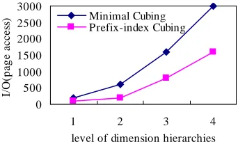
The performance results of prefix-index cubing and the minimal cubing of Li’s and Han’s[11] are reported from Fig. 2 to Fig. 5. Fig. 2 shows the storage size of the two methods on the cube had
T=106 tuples and h =1 level hierarchy and with shell fragment size f=3 , and the storage size of the two methods on the cube had h=3 levels hierarchies is shown in the Fig. 3. Fig. 4 shows the average I/O page access for online query of the two methods on the cube had different levels of hierarchy and with shell fragment size f=3 and T=106 tuples. Fig. 5 shows the average I/Os of prefix-index cubing method with different dimensions .
0 100 200 300 400 500
10 20 30 40
number of dimensions
st
o
rag
e s
iz
e(
M
B
) Minimal Cubing
[image:6.612.343.514.241.339.2]Prefix-index Cubing
Fig. 2. Storage size of shell segment with h=1
0 500 1000 1500 2000 2500 3000
10 20 30
number of dimensions
st
o
rag
e s
iz
e(
M
B
) Minimal Cubing
[image:6.612.339.510.383.485.2]Prefix-index Cubing
Fig. 3. Storage size of shell segment with h=3
0 500 1000 1500 2000 2500 3000
1 2 3 4
level of dimension hierarchies
I/
O
(p
ag
e a
cc
es
[image:6.612.343.511.524.625.2]s) Minimal CubingPrefix-index Cubing
Fig. 4. Average I/Os with f=3 and d=10
0 500 1000 1500 2000 2500 3000
1 2 3 4
level of dimension hierarchies
I/
O
(p
ag
e a
cc
es
s) D=10
D=20
Fig. 5. Average I/Os with f=3 of prefix-index cubing
6. CONCLUSION
systems and accelerating data mining tasks in large data warehouses. But in a high-dimensional hierarchical OLAP, it might not be practical to build all these cuboids and their indices In this paper, we propose a multi-dimensional hierarchical cubing algorithm, Prefix-index hierarchical cubing. It partitions a high dimensional cube into a set of disjoint low dimensional cubes. OLAP queries are computed online by dynamically constructing the cuboids from these cube segments. The analytical and experimental results show that proposed Prefix-index hierarchical cubing algorithm is significantly more efficient in time and space than the other leading cubing methods.
ACKNOWLEDGEMENTS
The research in the paper is supported by the National Natural Science Foundation of China under Grant No. 61070047, 61003180; the “Six Talent Peaks Program” of Jiangsu Province of China; the “333 Project” of Jiangsu Province of China.
REFERENCES
[1] S. Chauduri, and U. Dayal, “An overview of data warehousing and OLAP technology”,
SIGMOD Record, Vol. 26, No. 1,1997,pp.
65-74.
[2] K. Wu, E. J. Otoo, and A. Shoshani, “A performance comparison of bitmap indexes”,
Proceedings of the 10th International
Conference on Information and Knowledge
Management, ACM Press ,New York, NY,
2001, pp.559-561.
[3] H. Mistry, P. Roy, and S. Sudarshan, “Materialized view selection and maintenance using multi-query optimization”, Proceedings of
the 2001 ACM SIGMOD, ACM Press ,New
York, NY, 2001, pp. 307-318.
[4] J. Gray, S. Chaudhuri, A. Bosworth , A. Layman, D. Reichart, M. Venkatrao, F. Pellow, and H. Pirahesh. “Datacube: A relational aggregation operator generalizing group-by, cross-tab and subtotals”, Data Mining and Knowledge Discovery, 1997, pp. 29-54.
[5] K. Beyer, and R. Ramakrishnan, “Bottom-up computation of sparse and iceberg cubes”,
Proceedings of the 1999 ACM SIGMOD, ACM
Press ,New York, NY,1999, pp. 359-370. [6] J. Han, J. Pei, G. Dong, and K. Wang, “Efficient
computation of iceberg cubes with complex measures”, Proceedings of the 2001 ACM
SIGMOD , ACM Press ,New York, NY, 2001,
pp.1-12.
[7] L. V. S. Lakshmanan, J. Pei, and J, Han, “Quotient cubes: how to summarize the semantics of a data cube”, Proceedings of 28th International Conference on Very Large Data
Bases, Morgan Kaufmann, San Fransisco, 2002,
pp. 778-789.
[8] D. Xin, J. Han , X. Li, and B. W Wah, “Star-cubing:computing iceberg cubes by top-down and bottom-up integration”, Proceedings of 29th International Conference on Very Large
Data Bases ,Morgan Kaufmann, San Fransisco,
2003, pp. 476-487.
[9] L. V. S. Lakshmanan, J. Pei, and Y. Zhao, “QC-trees: An efficient summary structure for semantic OLAP”, Proceedings of the 2003
ACM SIGMOD ,ACM Press ,New York, NY,
2003, pp. 64-75.
[10]Y. Sismanis, A. Deligiannakis, Y. Kotidis, and N. Roussopoulos, “Hierarchical dwarfs for the rollup cube”, Proceedings of 30th International
Conference on Very Large Data Bases, Morgan
Kaufmann, San Fransisco, 2004, pp. 540-551. [11]X. Li, J. Han, and H. Gonzalez,
“High-dimensional OLAP: A minimal cubing approach”, Proceedings of 30th International
Conference on Very Large Data Bases . Morgan