THE PREDICTION OF GROUNDWATER LEVEL ON
TIDAL LOWLANDS RECLAMATION USING
EXTREME LEARNING MACHINE
1,2
NURHAYATI, 2INDRATMO SOEKARNO, 2IWAN K. HADIHARDAJA, 2M. CAHYONO 1Civil Engineering Department, University of Tanjungpura, Pontianak, Indonesia
2Civil Engineering Department, Institut Teknologi Bandung, Bandung, Indonesia
E-mail: [email protected], [email protected], [email protected], 2[email protected]
ABSTRACT
Groundwater level in the tidal lowlands fluctuates according to space and time. It is influenced by local rainfall or tidal. Tidal lowlands development for agriculture particularly food crops requires proper water management strategies so that the productivity of land and the production of food crops can be optimized. Proper water management must be supported by an accurate prediction system. This research aims to apply extreme learning machine (ELM) which can be used to make a prediction system of groundwater level in tidal lowlands. ELM is a feed forward artificial neural network with a single hidden layer or commonly referred to as single hidden layer feed forward neural networks (SLFNs). ELM has the advantage in learning speed. The result of the ground water level prediction using ELM was better than that using BPANN. Based on these results, the ELM can be used to predict the ground water level in order to assist decision makers in determining water management strategies and the determination of appropriate cropping patterns in the tidal lowlands reclamation.
Keywords: Prediction, Ground Water Level, Back Propagation, Artificial Neural Network, Extreme Learning Machine
1. INTRODUCTION
Water management is one of the keys to succeed in farming systems in tidal lowlands for agriculture particularly food crops. Water management in tidal lowlands faces some obstacles including water level fluctuations in farm land. Groundwater level information is obtained by making observations in the field but it takes time, cost and a lot of energy [1]. An accurate prediction system is required to obtain water level information.
There are many prediction methods used by the experts to get the correct prediction, one of which is a method based on artificial intelligence (AI). The most popular AI method used and the one that has been applied by experts [2], [3], [4] in this prediction is Back propagation of Artificial Neural Network (BPANN). BPANN has an advantage in control area, prediction and pattern recognition. Many researchers have concluded that BPANN is better than the conventional prediction methods [5].
AI method used in this research is the extreme learning machine (ELM). ELM is a new learning
method of neural network. ELM is a feed forward neural network with a single hidden layer or commonly referred to as single hidden layer feed forward neural networks (SLFNs) [5], [6], [7].
ELM has the advantage in the learning speed. Hence, by applying the ELM, it is expected to produce an accurate and effective prediction.
It is expected that the outcomes of groundwater level prediction research using ELM are better than those using BPANN and they can be used appropriately in determining water management strategies and the determination of cropping patterns on tidal lowlands reclamation in order to increase agricultural land productivity and crop productivity.
2. ARTIFICIAL NEURAL NETWORK (ANN)
human or biological neuron and it is based on the following assumptions: 1) Information processing occurs on many elements called neurons, 2) Signals run between neurons connected by network, 3) Each of connection network is associated with a weight, which is in a particular neural network, double the signal transmission, and 4) Each neuron uses activation function the (non-linear) to its input network to determine the output signal.
NN is characterized by: 1) The pattern is connected between neurons (called architecture), 2) Method to determine the weights of the connections (called training or learning algorithm of groundwater level), and 3) Activation function.
NN consists of a lot of processing elements called neurons, units, cells or nodes. Each neuron is connected to another by direct network communication tools and each is connected by weights. Weight portrays information used by the network to solve the problem. NN can be used to store, retrieve data or patterns repeatedly, classify pattern, perform general mapping from input patterns to output patterns, group similar patterns, or find an optimal solution for a problem.
Each neuron has an internal part called activation or activation level which function is to receive input. In particular, a neuron sends activation in the form of a signal to other neurons.
3. BACKPROPAGATION (BP)
BP is a descent gradient method to minimize the total square error of the output computed by the network. BP trains network to get a balance between the ability of the network to recognize the patterns used during the training process and the ability of the network to provide the correct response to the similar (but not identical) input pattern.
1). Architecture
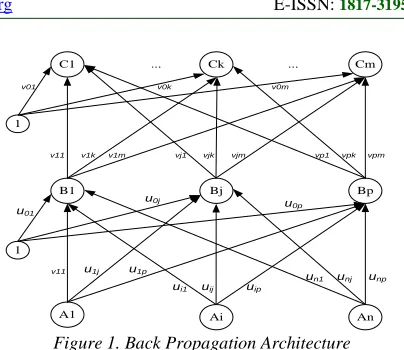
[image:2.612.317.519.80.255.2]BP has several units located in one or more hidden layers.
Figure 1 represents the architecture of BP with n inputs (plus a bias), a hidden layer consisting of p units (plus a bias), as well as m output units. Where
uij is the weight of a line from the input unit Ai to
hidden layer unit Bj (uj0 is the weight of the line
connecting bias in the input unit to the hidden layer unit Bj). vji is the weight from hidden layer unit Bj
to output unit Ck (vk0 is the weight of the line
connecting bias in the hidden layer unit to the output unit Bk).
C1 Ck Cm
B1 Bj Bp
A1 Ai An
1
1
... ...
u01
u0j u0p
u1j u
np
u1p u
n1 v11
uij
ui1
unj
uip v01 v0k
v1k v1m vj1 vjk vjm vp1 vpk vpm v0m
[image:2.612.314.525.466.624.2]v11
Figure 1.Back Propagation Architecture
2). Activation Function
Activation function for BP network has several important characteristics. Continuous activation function can be derived and it does not decrease monotonically. The derivative of the activation function is also easy to calculate for efficiency calculations. The most common activation function used is the value of derivatives (on the specific value of the independent variable) which can be expressed in terms of the value of the activation function (the value of the independent variable).
The activation function most often used is the binary sigmoid function while another function that is also quite often used is bipolar sigmoid function. Explanation of the two functions is given as follows:
a. A binary sigmoid function is for the interval (0,1)
( )
xe x
f −
+ =
1 1
(1)
( )
x f(
[
f( )
x]
)
f
1 1
' = − (2) b. A bipolar sigmoid function is for the interval
(-1,1)
( )
11 2
− − + = x
e x
f (3)
( )
x[
f
( )
x
]
[
f
( )
x
]
f
1
21
22 1
' =
+
−
(4)3). Algorithm of Back propagation water level
Step 0 : Initialize weights of all weights with small random numbers
Step 1 : If the termination condition is not met, do step 2-9
Step 2 : For each pair of training data, do steps 3-8
forwards them to the hidden unit Step 4 : Calculate all output in hidden unit Step 5 : Calculate all output in output unit Step 6 : Calculate δ units of output based on
the error in each output unit Ck
Step 7 : Calculate δ hidden units based on error in each hidden unit Bj
Step 8 : Calculate all the weight changes Step 9 : Test the termination conditions
4. EXTREME LEARNING MACHINE (ELM)
Extreme learning machine is a new learning method of neural network. ELM is a feedforward neural network with a single hidden layer or commonly referred to as single hidden layer feedforward neural networks (SLFNs) [5].
ELM learning method was created to overcome the weaknesses of feedforward artificial neural networks especially in terms of learning speed. There are two reasons why the feedforward artificial neural network has a low learning speed [5] [6] [7] [8] [9]: (1) Using a slow gradient based learning algorithm to do the training. All parameters on the network are determined iteratively by using that method of learning. (2) Learning using conventional gradient based learning algorithms, such as backpropagration (BP) and its variants, Lavenberg Marquadt (LM). All parameters of the feedforward artificial neural networks must be manually specified [6].
The parameters meant are the input weight and hidden bias. These parameters are also interconnected between one layer with another. Thus, it requires a long learning speed and it is often stuck in local minima [7], [9]. Input weight and hidden bias on the ELM are randomly selected so that ELM has a fast learning speed and it is able to produce good generalization performance. Figure 2 is the structure of the ELM.
ELM methods have a different mathematical model from feedforward artificial neural networks. The mathematical model of the ELM is simpler and more effective.
Mathematical model of the ELM to N number of different samples
(
Xi,Xt)
.[
]
nR T n Xi Xi Xi
Xi= 1, 2,, ∈ (5)
[
]
T RmXt Xt Xt
Xt= 1, 2,, m ∈ (6)
SLFNs standard with N number of hidden nodes and g(x)activation function can be described mathematically as follows:
( )
∑(
)
= + = ∑ = = N N i j o i b i X i W ig i j X igi ~ ~ 1 . 1 ββ (7)
Where: j=1,2,..., N; Wi =
(
Wi1,Wi2,,Win)
T = the vector of weight connecting i to the hidden nodesand input nodes;
β
i=(
β
i1,β
i2,,β
im)
T = the vector of weight connecting i to the hidden nodesand output nodes; bi= threshold of i to the hidden
nodes; WiXj= inner product of WiandXj.
SLFNs with N hidden nodes and g(x)activation function is assumed to be able to approximate with an error rate of 0 or it can be denoted as follows:
∑ = − = N j j t j o ~ 1
0 , so that oj =tj (8)
(
)
∑
= + =
N
j
i igWi X bi tj
~
1 .
β (9)
Equation (9) can be written simply as
T
H
β
= (10)(
wi w bi b xi xN)
H = , N~, , N~, , (11)
(
)
(
)
N Nx N b N x N w g b N x w g N b N x N w g b x w g H ~ ~ . ~ 1 . 1 ~ . ~ 1 1 . 1 + + + + = (12) =
T
N
T
β
β
β
1
(13)
=
T
N
T
T
T
T
1
(14)H in equation (12) above is the hidden layer output matrix. g
(
wi.xi +bi)
shows that the output of the hidden neurons related to the input of xi,β is the output weight matrix and T matrix of the target or output.associated with the hidden layer can be determined from equation (15).
T T H
=
[image:4.612.92.300.93.298.2]β (15)
Figure 2. Structure Of ELM [5]
5. IMPLEMENTATION OF THE
PROPOSED METHOD TO THE SYSTEM
Several stages to go through in the ground water level prediction using ELM are as follows:
[image:4.612.313.519.104.256.2]5.1.
Data Collection and Data ProcessingFigure 3. Location of Delta Telang I Lowlands Areas, South Sumatra Indonesia
The types of data used in this research are secondary data. Data used include rainfall, evapotranspiration, water level in the canal, hydraulic conductivity, and drain spacing. The source of data research is taken from the project Land and Water Management of Tidal Lowlands (LWMTL) 2005 and Strengthening Tidal Lowlands Development (STLD) 2007 in the district of Banyuasin, South Sumatra, Indonesia from April 2006 to June 2008.
Primary Canal (SP 5) Tertiary Canal 17
OT 4.5
OT 4.6 OT 4.4 OT 4.3
OT 4.2 OT 4.1 Tertiary Canal 4
Tertiary Canal 3 Tertiary Canal 1 Primary Canal (SP 6)
Secondary Canal
(
SDU
)
Secondary Canal
(
SPD
)
[image:4.612.93.285.374.531.2]Peilschaal Wells Water Gate
Figure 4. The Position Of The Groundwater Level And Water Level Canal Observations [1]
5.2.
Data DistributionTraining and testing process are absolutely necessary in the prediction process using ELM. Training process was used to develop a model of the ELM while testing was used to evaluate the ability of ELM as forecasting tool. Therefore the data were divided into two, namely the training data and the testing data. Data were shared with the ratio of 70:30, ie 70% for training and 30% for testing.
5.3.
ELM TrainingELM has to go through the training process first before it is being used as a tool to predict the groundwater level. The purpose of this process is to get input weight, bias and output weight with a low error rate.
5.4.
Data Training NormalizationData to be inputted to the ELM should be normalized so as to have a certain range of value. This is necessary because the activation function used will produce output with a range of data [0,1] or [-1,1]. Training data in this research are normalized so that they have the value range [-1,1]. The formula used in the normalization process.
{ }
(
)
{ } { }
(
)
1min max
min 2
− −
− × =
p X p
X
p X p
X X
(16)
Where: X= the value of the normalization result ranging between [-1,1]; Xp= the value of the
original data that have not been normalized;
( )
Xpmin = minimum value in the data set, and
( )
Xpmax = maximum value in the data set.
β
w
xi1 xi2 xin
Input layer Hidden layer Output layer
5.5.
Determining Activation Function and The Number of Hidden NeuronThe number of hidden neurons and the activation function in the training process should be determined in advance. On this research, trials using the log sigmoid activation function. In addition, linear transfer function was also used since the data predicted were stationary. Linear transfer function has a weakness in the data pattern that has a trend [4].
5.6.
Determining Weight Function, Bias of Hidden Neuron and Output WeightThe output of the ELM training process was the input and output weight as well as bias of the hidden neuron with a low error rate measured by the MSE and MAPE. Input weight was determined randomly while the output weight was the inverse of the matrix of hidden layer and output.
5.7.
Denormalization OutputThe output resulted from the training process was denormalized so that we obtained the predicted groundwater levels from training data. Denormalization formula used was:
(
Xp)
(
{ } { }
Xp Xp) { }
XpX=0,5× +1× max −min +min
(17)
Where: X = the data value after
denormalization; Xp = the output data before
denormalization; min
( )
Xp = minimum data on thedata sets before normalization; max
( )
Xp =maximum data on the data sets before normalization.
5.8.
Testing ELMBased on the input weight and output weight obtained from the training process, the next step is to predict the ground water level. The input data were normalized in advance using the same range and the same normalization formula with the training data. Automatically, the output of this process should also be normalized.
5.9.
The Analysis Prediction ResultsAfter going through various stages as described above, the prediction value of groundwater level was obtained. The results were then analyzed whether they had small error rates (MSE and
MAPE). If the resulting error rate is still relatively large, the steps that have been made will be re-evaluated, starting from the process of training and testing (predicting) until optimal results are obtained.
Mathematical formula of the mean square error (MSE) and mean absolute percentage error (MAPE).
n n
i
MSE
e
i /1 2
∑ =
= (18)
Where: ei = Xi −Fi
n n
i
MAPE
PE
i /1 ∑ =
= (19)
Where:
( )
100
−=
i X
i F i X i
PE
5.10.
Comparing Prediction Results of BPANN and ELMSTART Pre-Processing Data
Training
Testing
MAPE and MSE ≤ 5%
Data Denormalization
STOP
Input Weight, Bias and Output Weight
Input Weight, Bias and Output Weight
Groundwater Level Predicted Data Normalization
Training and Testing Data
[image:5.612.331.497.306.670.2]No Yes
Figure 5. Flowchart Of Training And Prediction Using ELM
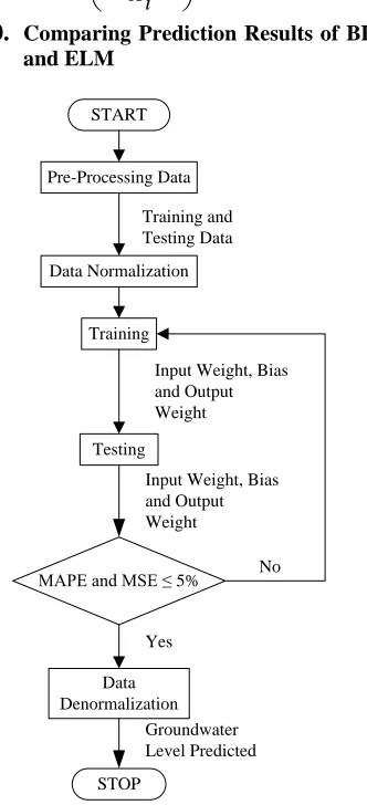
was done. The next step was to compare between the results of prediction of groundwater level with the result of the groundwater level as a result from the field observations. This was done to determine the accuracy level of the result of the groundwater level prediction using ELM with the groundwater level as a result from the observations in the field. Flowchart of training and prediction using ELM is shown in Figure 5.
6. RESULT AND ANALYSIS
The following are the prediction results of groundwater levels on tidal lowlands using BP-ANN and ELM. The activation function used on these two methods was sigmoid.
The data parameters used on BPANN are as follows:
Epoch = 100
Goal = 0.001
Max performance incremental = 1.05
Learning rate (Lr) = 0.01
Lr incremental = 1.05
Lr-decremental = 0.7
Momentum = 0.9
[image:6.612.317.523.111.258.2]The testing results (predictions) using ELM are as follows:
Figure 6. Groundwater Level OT4.1 As A Result From The Training Using ELM
[image:6.612.90.301.271.620.2]Figure 6 shows that the groundwater level OT4.1 as a result from training using ELM has a relatively small error rate value. It meant that the result of the training was the same as the result of the observation. Therefore, it can be concluded that the training on groundwater level was successful. The values of the error rate as a result of the training were as follows: MSE = 0.00027466, and MAPE = 0.9670%.
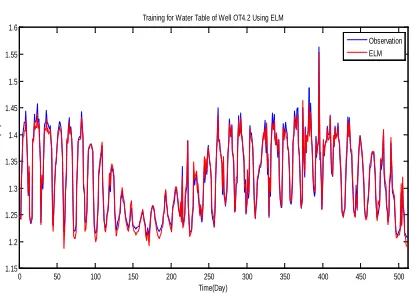
Figure 7. Groundwater Level OT4.2 As A Result From The Training Using ELM
[image:6.612.89.300.390.555.2]Figure 7 shows that the groundwater level OT4.2 as a result from training using ELM has a relatively small error rate value. It meant that the result of the training was the same as the result of the observation. Therefore, it can be concluded that the training on groundwater level was successful. The values of the error rate as a result of the training were as follows: MSE = 0.000068223, and MAPE = 0.5516%.
Figure 8. Groundwater Level OT4.3 As A Result From Training Using ELM
Figure 8 shows that the groundwater level OT4.3 as a result from training using ELM has a relatively small error rate value. It meant that the result of the training was the same as the result of the observation. Therefore, it can be concluded that the training on groundwater level was successful. The values of the error rate as a result of the training were as follows: MSE = 0.00025623, and MAPE = 0.9045%.
0 50 100 150 200 250 300 350 400 450 500 1.05
1.1 1.15 1.2 1.25 1.3 1.35 1.4 1.45 1.5
Training for Water Table of Well OT4.1 Using ELM
Time(Day)
E
lev
at
ion(
m
)
Observation ELM
0 50 100 150 200 250 300 350 400 450 500 1.15
1.2 1.25 1.3 1.35 1.4 1.45 1.5 1.55 1.6
Training for Water Table of Well OT4.2 Using ELM
Time(Day)
E
lev
at
ion(
m
)
Observation ELM
0 50 100 150 200 250 300 350 400 450 500 1.1
1.15 1.2 1.25 1.3 1.35 1.4 1.45 1.5
Training for Water Table of Well OT4.3 Using ELM
Time(Day)
E
lev
at
ion(
m
)
[image:6.612.313.522.406.544.2]Figure 9. Groundwater Level OT4.4 As A Result From Training Using ELM
[image:7.612.315.522.128.278.2]Figure 9 shows that the groundwater level OT4.4 as a result from training using ELM has a relatively small error rate value. It meant that the result of the training was the same as the result of the observation. Therefore, it can be concluded that the training on groundwater level was successful. The values of the error rate as a result of the training were as follows: MSE = 0.000052688, and MAPE = 0.4461%.
Figure 10. Groundwater Level OT4.5 As A Result From Training Using ELM
Figure 10 shows that the groundwater level OT4.5 as a result from training using ELM has a relatively small error rate value. It meant that the result of the training was the same as the result of the observation. Therefore, it can be concluded that the training on groundwater level was successful. The values of the error rate as a result of the training were as follows: MSE = 0.00030391, and MAPE = 1.0206%.
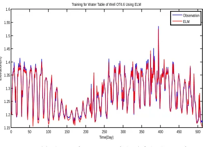
Figure 11. Groundwater Level OT4.6 As A Result From Training Using ELM
Figure 11 shows that the groundwater level OT4.6 as a result from training using ELM has a relatively small error rate value. It meant that the result of the training was the same as the result of the observation. Therefore, it can be concluded that the training on groundwater level was successful. The values of the error rate as a result of the training were as follows: MSE = 0.000059577, and MAPE = 0.4905%.
The result of the groundwater level prediction using ELM was as follows:
Figure 12. Groundwater Level OT4.1 As A Result From Prediction Using ELM
Figure 12 shows that the groundwater level as a result from prediction on OT4.1 using ELM has a relatively small error rate value. It meant that the result of the prediction was the same as the result of observation. Therefore, it can be concluded that the prediction on groundwater level was successful. The values of the error rate as a result of the prediction were shown completely as follows: MSE = 0.00034573, and MAPE = 1.0238%.
0 50 100 150 200 250 300 350 400 450 500 1.15
1.2 1.25 1.3 1.35 1.4 1.45 1.5 1.55 1.6
Training for Water Table of Well OT4.4 Using ELM
Time(Day)
E
lev
at
ion(
m
)
Observation ELM
0 50 100 150 200 250 300 350 400 450 500 1.05
1.1 1.15 1.2 1.25 1.3 1.35 1.4 1.45 1.5
Training for Water Table of Well OT4.5 Using ELM
Time(Day)
E
lev
at
ion(
m
)
Observation ELM
0 50 100 150 200 250 300 350 400 450 500 1.15
1.2 1.25 1.3 1.35 1.4 1.45 1.5 1.55 1.6
Training for Water Table of Well OT4.6 Using ELM
Time(Day)
E
lev
at
ion(
m
)
Observation ELM
0 20 40 60 80 100 120 140 160 180 200 1.1
1.15 1.2 1.25 1.3 1.35 1.4 1.45 1.5
Prediction for Water Table of Well OT4.1 Using ELM
Time(Day)
E
lev
at
ion(
m
)
[image:7.612.92.301.407.552.2] [image:7.612.316.523.446.587.2]Figure 13. Groundwater Level OT4.2 As A Result From Prediction Using ELM
[image:8.612.314.523.420.557.2]Figure 13 shows that the ground water level as a result from prediction on OT4.2 using ELM has a relatively small error rate value. It meant that the result of the prediction was the same as the result of observation. Therefore, it can be concluded that the prediction on groundwater level was successful. The values of the error rate as a result of the prediction were as follows: MSE = 0.000068923, and MAPE = 0.4653%.
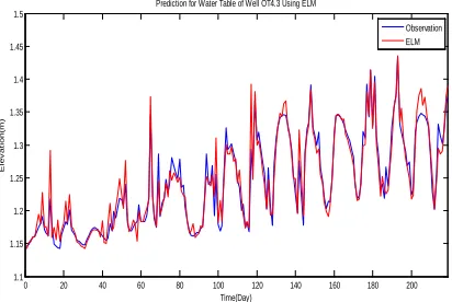
Figure 14. Groundwater Level OT4.3 As A Result From Prediction Using ELM
Figure 14 shows that the groundwater level as a result from prediction on OT4.3 using ELM has a relatively small error rate value. It meant that the result of the prediction was the same as the result of observation. Therefore, it can be concluded that the prediction on groundwater level was successful. The values of the error rate as a result of the prediction were as follows: MSE = 0.00031283, and MAPE = 0.9647%.
Figure 15. Groundwater Level OT4.4 As A Result From Prediction Using ELM
[image:8.612.93.299.427.565.2]Figure 15 shows that the ground water level as a result from prediction on OT4.4 using ELM has a relatively small error rate value. It meant that the result of the prediction was the same as the result of observation. Therefore, it can be concluded that the prediction on groundwater level was successful. The values of the error rate as a result of the prediction were as follows: MSE = 0.000070310, and MAPE = 0.4628%.
Figure 16. Groundwater Level OT4.5 As A Result From Prediction Using ELM
Figure 16 shows that the ground water level as a result from prediction on OT4.5 using ELM has a relatively small error rate value. It meant that the result of the prediction was the same as the result of observation. Therefore, it can be concluded that the prediction on groundwater level was successful. The values of the error rate as a result of the prediction were as follows: MSE = 0.00031845, and MAPE= 0.9870%.
0 20 40 60 80 100 120 140 160 180 200 1.25
1.3 1.35 1.4 1.45 1.5 1.55 1.6
Prediction for Water Table of Well OT4.2 Using ELM
Time(Day)
E
lev
at
ion(
m
)
Observation ELM
0 20 40 60 80 100 120 140 160 180 200 1.1
1.15 1.2 1.25 1.3 1.35 1.4 1.45 1.5
Prediction for Water Table of Well OT4.3 Using ELM
Time(Day)
E
lev
at
ion(
m
)
Observation ELM
0 20 40 60 80 100 120 140 160 180 200 1.25
1.3 1.35 1.4 1.45 1.5 1.55
Prediction for Water Table of Well OT4.4 Using ELM
Time(Day)
E
lev
at
ion(
m
)
Observation ELM
0 20 40 60 80 100 120 140 160 180 200 1.1
1.15 1.2 1.25 1.3 1.35 1.4 1.45 1.5
Prediction for Water Table of Well OT4.5 Using ELM
Time(Day)
E
lev
at
ion(
m
)
Figure 17. Groundwater Level OT4.6 As A Result From Prediction Using ELM
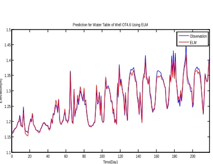
Figure 17 shows that the ground water level as a result from prediction on OT4.6 using ELM has a relatively small error rate value. It meant that the result of the prediction was the same as the result of observation. Therefore, it can be concluded that the prediction on groundwater level was successful. The values of the error rate as a result of the prediction were as follows: MSE = 0.000074588, and MAPE = 0.5062%.
Comparison of the results of the ground water level prediction using ELM and BPANN can be seen in Table 1.
Table 1. Comparison Of The Results Of The Ground Water Level Using ELM And BPANN For OT4.1, OT4.3,
OT4.5 Simulation BPANN OT4.1,
OT4.3, OT4.5
ELM OT4.1, OT4.3, OT4.5 Training time 19.5156 2.7813 MSE training 0.00035595 0.0002726 MAPE training 1.0212 0.9640 Testing time 0.1406 0.0781 MSE testing 0.0012 0.00032567 MAPE testing 1.8600 0.9918
Table 2. Comparison Of The Results Of The Ground Water Level Using ELM And BPANN For OT4.2, OT4.4,
OT4.6 Simulation BPANN OT4.2,
OT4.4, OT4.6
[image:9.612.91.300.115.276.2]ELM OT4.2, OT4.4, OT4.6 Training time 20.1563 2.6719 MSE training 0.00041518 0.000060163 MAPE training 0.5120 0.4828 Testing time 0.1875 0.0469 MSE testing 0.0012 0.000071274 MAPE testing 1.7249 0.4781
Table 1 and Table 2 show that the comparison of the level of training error and prediction error on groundwater level prediction using ELM is smaller than that using BPANN. The time of the training process and the prediction process on groundwater level using ELM is faster than that using BPANN.
Table 1 and Table 2 show that the result of training and prediction using ELM and BPANN is able to work well in recognizing input data given to the system because the error rate is relatively small. The result of training and prediction using ELM is better than those using BPANN.
7. CONCLUSION
ELM proposed in this paper is used to predict the ground water level in the tidal lowlands reclamation in Indonesia. The method used in this paper is ELM while BPANN is used as validation. The result shows that the training result and the groundwater level prediction using ELM are better than those using BPANN.
ACKNOWLEDGEMENTS
The authors would like to thank the Government of Indonesia, especially Directorate General of Higher Education for Postgraduate Scholarship (BPPS), University Tanjungpura for University Decentralization Research on Doctoral Dissertation Grant during research that we receive, Water Resources Engineering Laboratory, Civil Engineering Faculty, Institut Teknologi Bandung (ITB), Bandung Indonesia for all the facilities provided for this research.In addition, the authors would like to express their gratitude to the project Land and Water Management of Tidal Lowlands (LWMTL) 2005 and Strengthening Tidal Lowlands Development (STLD) 2007 in the district of Banyuasin, South Sumatra, Indonesia for the willingness of giving out the data and permission for publication.
REFRENCES:
[1] Ngudiantoro, Hidayat Pawitan, Muhammad Ardiansyah, M. Yanuar J. Purwanto, Robiyanto H. Susanto Modeling of Water Table Fluctuation on Tidal Lowlands Area of B/C Type: A Case in South Sumatra, Forum
Pascasarjana, Vol. 33, No. 2, April 2010, pp.
101-112.
[2] Jianhui Wu, Qi Ren, Yu Su, Sufeng Yin, Houjun Xu, Guoli Wang, Study and Application of Combination Prediction Model
0 20 40 60 80 100 120 140 160 180 200 1.1
1.15 1.2 1.25 1.3 1.35 1.4 1.45 1.5
Prediction for Water Table of Well OT4.6 Using ELM
Time(Day)
E
lev
at
ion(
m
)
of Principal Component Analysis and BP Neural Network, Journal of Theoretical and
Applied Information Technology, Vol. 49, No.
3, March 31, 2013, pp. 798-804.
[3] Xianghong Wang, Jianhui Wu, Sufeng Yin, Zhengjun Guo, Guoli Wang, Research on Combined Prediction Model Based on BP Neural Network and its Application, Journal of Theoretical and Applied Information
Technology, Vol. 49, No. 3, March 31, 2013,
pp. 783-789.
[4] Guoqiang Zang, B. Eddy Patuwo, Michael Y. Hu, Forecasting with Artificial Neural Networks: The State of the Art, International
Journal of Forecasting, 14 (1998), 35-62.
[5] Zhan-Li Sun, Tsan-Ming Choi, Kin-Fan Au, and Yong Yu, “Sales Forecasting Using Extreme Learning Machine with Application in Fashion Retailing”, Decision Support Systems, Vol. 46, 2008, pp. 411-419.
[6] Guang-Bin Huang, Qin-Yu Zhu, and Chee-Kheong Siew, “Extreme Learning Machine: A New Learning Scheme of Feedforward Neural Networks”, in Proceedings of International Joint Conference on Neural Networks
(IJCNN), Budapest (Hungary), Vol. 2, July 25-29, 2004, pp. 985–990,
[7] Agus Widodo, Novitasari Naomi, Suharjito, Fredy Purnomo, Prediction of research topics using combination of machine learning and logistic curve, Journal of Theoretical and
Applied Information Technology, March 31,
2013, Vol. 49, No. 3, pp. 725–732.
[8] Guang-Bin Huang, Qin-Yu Zhu, Chee-Kheong Siew, “Extreme Learning Machine: Theory and Applications”, Neurocomputing, Vol. 70, 2006, pp. 489-501.
[9] Guang-Bin Huang and Chee-Kheong Siew, “Extreme Learning Machine with Randomly Assigned RBF Kernels”, International Journal
of Information Technology, 11(1), 2005, pp.
![Figure 4. The Position Of The Groundwater Level And Water Level Canal Observations [1]](https://thumb-us.123doks.com/thumbv2/123dok_us/8914541.961095/4.612.93.285.374.531/figure-position-groundwater-level-water-level-canal-observations.webp)