Analysis, classification and
management of insulin
sensitivity variability in a
glucose-insulin system model
for critical illness
Christopher Pretty
A thesis submitted for the degree of
Doctor of Philosophy
in
Mechanical Engineering
at the
University of Canterbury,
Christchurch, New Zealand
Acknowledgements
I would like to thank a number of people who have made my time working on this research for the past few years a rewarding experience.
To my supervisors, Prof. Geoff Chase and Dr. Geoff Shaw, for their enthusiasm, optimism, inspiration and guidance.
To Jessica Lin and Aaron Le Compte for their guidance, patience, knowledge and friendship.
To Fatanah, Matt, Ummu, Ash, Normy and Paul in the Centre for BioEngineering, for your friendship and making the work environment enjoyable and productive.
i
Contents
ABSTRACT ... XII
CHAPTER 1. INTRODUCTION... 1
1.1 AETIOLOGY OF HYPERGLYCAEMIA IN CRITICAL CARE ... 2
1.2 GLYCAEMIC CONTROL IN CRITICAL CARE ... 3
1.3 MODEL-BASED GLYCAEMIC CONTROL ... 5
1.4 PREFACE ... 6
CHAPTER 2. BACKGROUND ... 9
2.1 MODELLING AND PHYSIOLOGY ... 9
2.2 ROLE OF SI IN MODEL-BASED CONTROL ... 13
CHAPTER 3. ENDOGENOUS INSULIN SECRETION MODEL ... 15
3.1 INTRODUCTION ... 15
3.2 SUBJECTS AND METHODS ... 16
3.2.1 Patients and samples ... 16
3.2.2 Analysis methods ... 18
3.3 RESULTS AND DISCUSSION ... 19
3.3.1 Calculated endogenous secretion rates ... 19
3.3.2 Secretion rate bounds... 20
3.3.3 Model fitting ... 21
3.3.4 Model validation ... 23
3.3.5 Limitations ... 24
3.3.6 Impact on SI ... 25
3.4 SUMMARY ... 26
CHAPTER 4. INTERSTITIAL INSULIN KINETICS ... 27
4.1 INTRODUCTION ... 27
4.2 SUBJECTS AND METHODS ... 28
4.2.1 Patients ... 28
4.2.2 Fitting and prediction grid search analysis ... 29
4.2.3 Microdialysis analysis ... 30
4.3 RESULTS AND DISCUSSION ... 32
4.3.1 Fitting and prediction grid-search results ... 32
4.3.2 Microdialysis results ... 33
4.3.3 Comparison of results ... 37
4.3.4 Impact on SI ... 39
ii
CHAPTER 5. ENDOGENOUS GLUCOSE PRODUCTION ... 41
5.1 INTRODUCTION ... 41
5.1.1 Background ... 42
5.2 SUBJECTS AND METHODS ... 43
5.2.1 Patients and samples ... 43
5.2.2 Analysis methods ... 44
5.3 RESULTS AND DISCUSSION ... 46
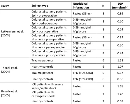
5.3.1 EGP from the literature ... 46
5.3.2 EGP as a function of BG... 48
5.3.3 EGP as a function of time ... 50
5.3.4 EGP in control during special circumstances ... 54
5.4 SUMMARY ... 55
CHAPTER 6. ICING-2 MODEL SUMMARY ... 56
6.1 INTRODUCTION ... 56
6.2 PHARMACOKINETIC-PHARMACODYNAMIC MODEL AND PARAMETERS ... 56
CHAPTER 7. PATIENT TYPE AND CONDITION ... 58
7.1 INTRODUCTION ... 58
7.2 SUBJECTS AND METHODS ... 59
7.2.1 Patients ... 59
7.2.2 Analyses: ... 60
7.3 RESULTS ... 61
7.3.1 Twenty-four hour analyses: ... 61
7.3.2 Six hour analyses: ... 64
7.3.3 Cardiovascular surgery patients ... 67
7.4 DISCUSSION ... 68
7.4.1 Insulin sensitivity variability ... 68
7.4.2 Reducing the impact of SI variability on outcome glycaemia ... 70
7.5 SUMMARY ... 72
CHAPTER 8. DRUG THERAPIES ... 73
8.1 INTRODUCTION ... 73
8.2 SUBJECTS AND METHODS ... 74
8.2.1 Glucocorticoid study subjects ... 75
8.2.2 Metoprolol study subjects ... 76
8.2.3 Analyses ... 77
8.3 RESULTS ... 79
8.3.1 Glucocorticoid analysis ... 79
iii
8.4 DISCUSSION ... 84
8.4.1 Glucocorticoids ... 84
8.4.2 Metoprolol... 86
8.4.3 Impact of drug therapies on SI and outcome glycaemia ... 87
8.5 SUMMARY ... 89
CHAPTER 9. MEASUREMENT ERRORS ... 90
9.1 INTRODUCTION ... 90
9.2 SUBJECTS AND METHODS ... 91
9.2.1 Patients ... 91
9.2.2 Error modelling ... 92
9.2.3 Analyses ... 94
9.3 RESULTS AND DISCUSSION ... 96
9.3.1 Timing error ... 96
9.3.2 Blood glucose measurement error ... 97
9.3.3 Combined measurement error ... 98
9.3.4 Implications of results ... 99
9.4 SUMMARY ... 101
CHAPTER 10. MODEL VALIDATION ... 103
10.1 INTRODUCTION ... 103
10.2 SUBJECTS AND METHODS ... 104
10.2.1 Patients ... 104
10.2.2 Glucontrol protocols... 106
10.2.3 Fitting and prediction ... 108
10.2.4 Self and cross-validation ... 108
10.3 RESULTS AND DISCUSSION ... 110
10.3.1 Fitting and prediction validation ... 110
10.3.2 Self and cross validation ... 111
10.4 SUMMARY ... 116
CHAPTER 11. IMPLEMENTATION VALIDATION ... 118
11.1 INTRODUCTION ... 118
11.2 SUBJECTS AND METHODS ... 119
11.2.1 Patients ... 119
11.2.2 Virtual trial simulation ... 120
11.2.3 STAR protocol ... 120
11.2.4 Analyses ... 122
11.3 RESULTS AND DISCUSSION ... 122
iv
CHAPTER 12. CONCLUSIONS ... 127
CHAPTER 13. FUTURE WORK ... 131
13.1 GASTRIC MODEL ... 131
13.2 INSULIN DELIVERY METHOD ... 131
13.3 HIGH FREQUENCY BG MEASUREMENTS ... 132
13.4 ENDOGENOUS INSULIN SECRETION AND GLUCOSE PRODUCTION ... 132
v
List of Figures
Figure 2.1. Schematic diagram of the ICING compartment model showing the compartments, kinetics and dynamics, appearance and clearance. ... 11
Figure 2.2. BG forecasting based on a stochastic model of SI. ... 13
Figure 3.1 Pre-hepatic insulin secretion plotted against each of the measured variables. Data indicating patients with an impaired insulin response to hyperglycaemia are shown in red. ... 19
Figure 3.2 Mean dose-response relationship between plasma glucose and pre-hepatic insulin secretion rates of healthy subjects during graded glucose infusion with a GLP-1 dose of 2.0 pmol/kg.min. [Kjems et al. 2003]. ... 20
Figure 3.3 Pre-hepatic insulin secretion data and 1-dimensional model fits. Non-diabetic data and model shown in blue (R2 = 0.61); T2DM data and model shown in red (R2 = 0.69). ... 22
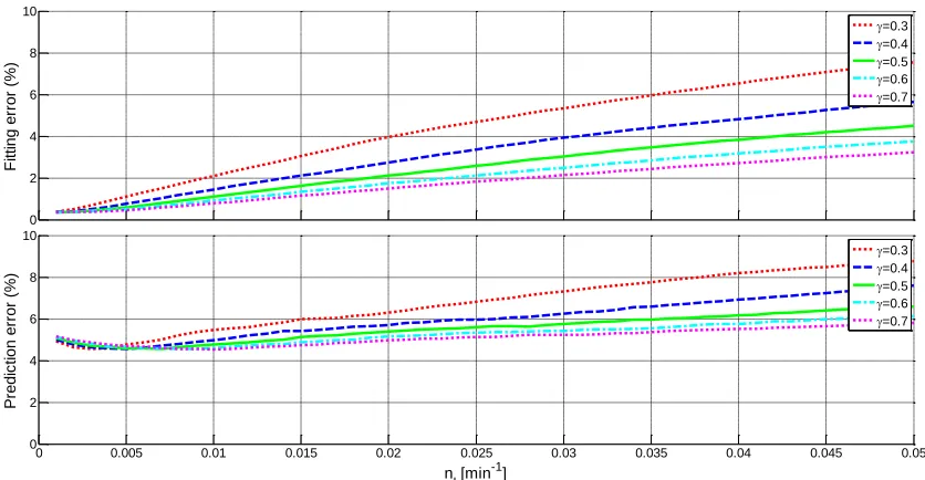
Figure 4.1 Fitting (top) and 1-hour-ahead prediction (bottom) errors (%) for the STAR-Liege cohort across a range of nI and γvalues. ... 32
Figure 4.2 Fitting (top) and 1-hour-ahead prediction (bottom) errors (%) for the Christchurch ICU sepsis cohort across a range of nI and γ values. ... 33
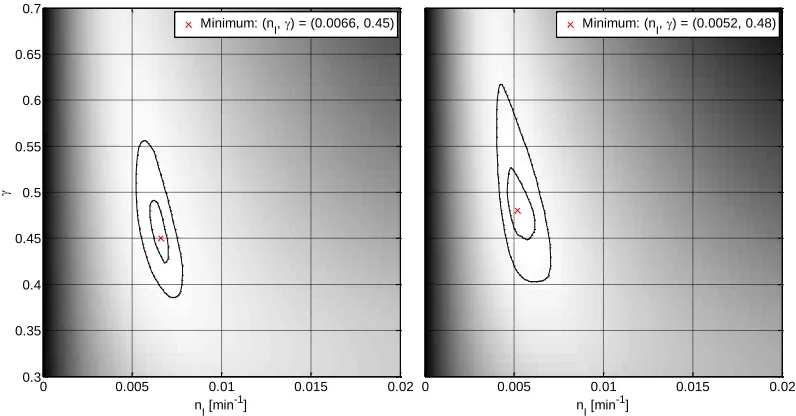
Figure 4.3 Grid-search error results from microdialysis analysis showing optimal parameter values. The left panel shows the results where each error value was weighted equally, and the right panel shows the results where each study was weighted equally. Contours are at error 1% and 5% greater than the minimum. Lighter areas represent lower error and darker areas, greater. ... 34
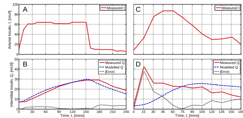
Figure 4.4 Two contrasting examples from the simulation of microdialysis data using the selected parameter set, nI =0.0060 min-1, γ= 0.5. The panels on the left show a good model fit to
measured data from Castillo et al. [1994] (body fat 13-21%). The panels on the right show a poor fit from Herkner et al. [2003] (OGTT). The upper panels present plasma insulin concentrations and the lower panels measured and modelled interstitial insulin
concentrations. ... 36
Figure 5.1 Schematic plot of proposed EGP(G) function. ... 45
Figure 5.2 Results of the EGP(G) shape optimisation based on BG fitting error over 48 hours using 10 cohorts of 20 SPRINT patients. ... 49
Figure 5.3 Time course of the number of instances where the fitted SI parameter was constrained to non-negative values during the first 48 hours of SPRINT. The top panel shows the results for the 200 patient SPRINT > 48 hours cohort. The bottom panel shows the 10 patient poor fit cohort. ... 51
Figure 5.4 Time course of minimum EGP values required to prevent non-physiologic negative fitted SI values for the poor fit cohort. The whiskers indicate the full range of EGP values. The model is fitted to the 75th-percentile points r2 = 0.87. ... 52
Figure 7.1. Insulin sensitivity level analyses by cohort (left) and per-patient median (right) using 24-hour blocks of data. ... 62
vi
Figure 7.3. Insulin sensitivity level analyses by cohort (left) and per-patient median (right) using 6-hour blocks of data. ... 65
Figure 7.4. Insulin sensitivity variability analyses by cohort (hour-to-hour percentage change) and per-patient interquartile-range using 6-hour blocks of data. ... 66
Figure 7.5. Insulin sensitivity level analyses by cohort (left) and per-patient median (right) for cardiovascular surgery patients. The grey lines show the data from the full 164 patient cohort for comparison. ... 68
Figure 7.6. Insulin sensitivity variability analyses by cohort (left) and per-patient median (right) for cardiovascular surgery patients. The grey lines show the data from the full 164 patient cohort for comparison. ... 68
Figure 8.1. CDFs of SI level for the control and steroid cohorts. The left panel shows the overall cohort comparison. The right panel shows the 25th-, 50th- and 75th percentile patients. ... 80
Figure 8.2. CDFs of SI hour-to-hour variability for the control and steroid cohorts. The left panel shows the overall cohort comparison. The right panel shows the 25th-, 50th- and 75th
percentile patients (top to bottom). ... 81
Figure 8.3. CDFs of SI level for the control and metoprolol cohorts. The left panel shows the overall cohort comparison. The right panel shows the 25th-, 50th- and 75th percentile patients. ... 82
Figure 8.4. CDFs of SI hour-to-hour variability for the control and metoprolol cohorts. The left panel shows the overall cohort comparison. The right panel shows the 25th-, 50th- and 75th
percentile patients (top to bottom). ... 83
Figure 9.1. Timing error models based on data from the STAR pilot trials [Evans et al. 2011]. Errors from 1-hour measurements are shown on the left and 2-hour measurements on the right. 93
Figure 9.2. SI level comparison method for the Monte Carlo simulations with added sensor and timing error. The width of the IQR of differences, expressed as percentages, was used to characterise the variability in level induced by the errors. ... 95
Figure 9.3. The impact of timing error on SI level (left panel) and variability (right panels),
characterised by the variability of these parameters determined by Monte Carlo simulation. The panels on the right show the location of the median simulated variability, compared to the actual (top) and the variability about that median (bottom). ... 97
Figure 9.4. The impact of BG sensor error on SI level (left panel) and variability (right panels), characterised by the variability of these parameters determined by Monte Carlo simulation. The panels on the right show the location of the median simulated variability, compared to the actual (top) and the variability about that median (bottom). ... 98
Figure 9.5. The impact of combined timing and BG sensor error on SI level (left panel) and
variability (right panels), characterised by the variability of these parameters determined by Monte Carlo simulation. The panels on the right show the location of the median simulated variability, compared to the actual (top) and the variability about that median (bottom). ... 99
Figure 10.1. SI level (left panel) and hour-to-hour variability (right panel) distributions of SPRINT and Glucontrol patients. ... 106
Figure 10.2. Distributions of blood glucose results of clinical Glucontrol data and virtual trials on a cohort basis. ... 111
vii
Figure 10.4. Per-patient median absolute BG comparison between simulated and clinical results. 113
Figure 11.1.Controller forecast schematic for BG targeting the range 4.4 – 8.0 mmol/L. A BG measurement was taken at 4 hours, and forecasts of BG have been generated (points A-F) for 1-3 hours ahead using the 5th and 95th percentile SI values from the stochastic model
and some possible insulin and nutrition intervention. ... 121
Figure 11.2. Comparison of 0-24hr and general stochastic models generated from the ICING-2 model. ... 123
Figure 11.3. Virtual trial simulation BG results during the first 24 hours of ICU stay. The
viii
List of Tables
Table 2.1 Parameter values and descriptions for the ICING model. ... 10
Table 2.2 Exogenous input variables to the ICING model... 11
Table 3.1 Summary of patient characteristics. Data are shown as median [IQR] where appropriate. ... 16
Table 3.2 Summary of patient diagnoses. ... 17
Table 3.3 Coefficients for endogenous insulin secretion models fitted with 1, 2 and 3 independent variables (dimensions). ... 21
Table 3.4 Glucose coefficient data from the literature. Results have been converted to the units of measurement used in this study where necessary. Assumptions used for these conversions were: w = 80 kg; BSAlean = 1.8 m2; BSAobese/T2DM = 2.1 m2. ... 24
Table 4.1 Summary of patient characteristics. Data are shown as median [IQR] where appropriate. ... 29
Table 4.2 Published microdialysis studies used to investigate interstitial insulin kinetic parameters ... 31
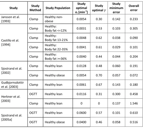
Table 4.3 Individual results from published microdialysis studies. Study minimum error is associated with the study optimal nI and γ. Overall error is associated with the selected parameter set,
nI =0.0060 min-1, γ= 0.5. The errors are unitless and represent mean absolute fractional
error at each measurement point. ... 35
Table 5.1 Summary of patient characteristics. Data are shown as median [IQR] where appropriate. ... 43
Table 5.2 EGP values measured in critically ill patients and healthy controls from the literature. Where reported values were normalised by anthropomorphic data, 80 kg and 1.8 m2 body
surface area have been in this table. Abbreviations; Epi: Epidural block; N. anaes: Normal anaesthesia; TPN: Total parenteral nutrition; CHO: carbohydrate; IV: intravenous. ... 47
Table 6.1 Parameter values and descriptions for the ICING-2 model. ... 57
Table 6.2 Exogenous input variables to the ICING-2 model. ... 57
Table 7.1. Summary details of the study subjects. The CVS patients are also included in the ICU cohort. Data are presented as median [interquartile range] where appropriate. ... 60
Table 7.2. Increasing cohort and per-patient median insulin sensitivity over time (24hr blocks). P-values calculated using Wilcoxon rank-sum test. ... 62
Table 7.3. Proportion of patients for whom median insulin sensitivity increases between the days indicated in the rows and columns. ... 63
Table 7.4. Reductions in the IQR and median per-patient range of hour-to-hour percentage insulin sensitivity change over time. P-values calculated using Kolmogorov-Smirnov test for cohort comparisons and Wilcoxon rank-sum test for per-patient comparisons. ... 64
ix
Table 7.6. Proportion of patients for whom median insulin sensitivity increases between the blocks indicated in the rows and columns. ... 66
Table 7.7. Reductions in the IQR and median per-patient range of hour-to-hour percentage insulin sensitivity change over time. P-values calculated using Kolmogorov-Smirnov test for cohort comparisons and Wilcoxon rank-sum test for per-patient comparisons. ... 67
Table 8.1. Glucocorticoid analysis cohorts. Data are shown as median [interquartile range] where appropriate. P-values were calculated using Fisher’s exact test for categorical data and the Wilcoxon rank-sum test for continuous data... 75
Table 8.2. Glucocorticoids and their properties used in this study [Derendorf et al. 1993; Melby 1977; Schimmer & Parker 2006]. ... 76
Table 8.3. Metoprolol analysis cohorts. Data are shown as median [interquartile range] where appropriate. P-values were calculated using Fisher’s exact test for categorical data and the Wilcoxon rank-sum test for continuous data... 77
Table 9.1. Cohort details summary. Data are shown as median [interquartile range] where
appropriate. ... 91
Table 9.2. Error components of the Arkray Super-Glucocard II glucometer [Arkray 2007]. ... 94
Table 10.1. Glucontrol cohort characteristics. Data are shown as median [interquartile range] where appropriate. P-values were calculated using the Chi-squared test and Wilcoxon rank-sum test. ... 105
Table 10.2. Clinical glucose control characteristics. Data are shown as median [interquartile range] where appropriate. ... 105
Table 10.3. Glucontrol A protocol. The starting insulin infusion rate is shown in the top part of the table. The maintenance infusion rates or increments are shown in the lower part. All values have been converted to mmol/L from mg/dL. ... 107
Table 10.4. Glucontrol B protocol. The starting insulin infusion rate is shown in the top part of the table. The maintenance infusion rates or increments are shown in the lower part. All values have been converted to mmol/L from mg/dL. ... 107
Table 10.5. Fitting and one-hour-ahead prediction errors for Glucontrol populations with ICING-2 model. Data are shown as median [interquartile range]... 110
Table 10.6. Glucontrol A clinical and simulation results. Data are shown as median [interquartile range] where appropriate. ... 114
Table 10.7. Glucontrol B clinical and simulation results. Data are shown as median [interquartile range] where appropriate. ... 115
Table 11.1. Cohort and sub-cohort summary statistics. ... 119
Table 11.2. Virtual trial simulation BG results comparison for data within 24 hours of ICU
admission. ... 124
x
Nomenclature
Acronyms and abbreviations
ACCP American College of Chest Physicians ACE Angiotensin-Converting Enzyme
APACHE Acute Physiological And Chronic Health Evaluation ARB Angiotensin II Receptor Blockers
AUCQ Area Under the interstitial insulin Concentration curve
BG Blood Glucose BGA Blood Gas Analyser BSA Body Surface Area
CDF Cumulative Distribution Function CGM Continuous Glucose Monitoring
CHO Carbohydrate
Clamp Euglycaemic-insulinaemic clamp CV Coefficient of Variation
CVS Cardiovascular Surgery
EGP Endogenous Glucose Production EIC Euglycaemic-insulinaemic clamp Epi Epidural block
GLP-1 Glucagon-Like Peptide-1
ICING Intensive Control Insulin-Nutrition-Glucose ICU Intensive Care Unit
IQR Interquartile Range ISR Insulin Secretion Rate IV Intravenous
N. Anaes Normal anaesthesia ND Non-Diabetic
OGTT Oral Glucose Tolerance Test
PK-PD Pharmacokinetic-Pharmacodynamic
SI Insulin sensitivity parameter
SIRS Systemic Inflammatory Response Syndrome SPRINT Specialised Relative Insulin and Nutrition Tables STAR Stochastic TARgeted
xii
Abstract
Hyperglycaemia in critical care is common and has been linked to increased mortality and morbidity. Tight control of blood glucose concentrations to more normal levels can significantly reduce the negative outcomes associated with hyperglycaemia. However, hypoglycaemia and glycaemic variability have also been independently shown to increase mortality in critically ill patients. Further complicating the matter, critically ill patients exhibit high inter- and intra patient metabolic variability and thus consistent, safe control of glycaemia has proved very difficult.
Model-based and model-derived tight glycaemic control methods have shown significant ability to provide very tight control with little or no hypoglycaemia in the intensive care unit (ICU). The model-based control practised in the Christchurch Hospital ICU uses a physiological model that relies on a single, time-varying parameter, SI, to capture the patient-specific glycaemic response to insulin. As an identified parameter, SI is prone to also capturing other, unintended, dynamics that add variability on multiple timescales. The objective of this research was to enable enhanced glycaemic control by addressing this variability of the SI parameter through better modelling and implementation.
An improved model of insulin secretion as a function of blood glucose concentration was developed using data collected from a recent study at the Christchurch Hospital ICU. Separate models were identified for non-diabetic patients and diagnosed, or suspected type II diabetic patients, with R2 = 0.61 and 0.69, respectively. The gradients of the functions identified were comparable to data published in a number of other studies on healthy and diabetic subjects.
xiii
Models of endogenous glucose production (EGP), as functions of blood glucose concentration and time, were assessed. These models proved unsatisfactory due to difficulties in identifying reliable functions with the available data set. Thus, it was determined that EGP should continue to be treated as a population constant, except during real-time glycaemic control, where the value may be adjusted temporarily to ensure valid SI values.
The first 24 hours of ICU stay proved to be a period of significantly increased SI
variability, both in terms of hour-to-hour changes and longer-term evolution of level. This behaviour was evident for the entire study cohort as a whole and was particularly pronounced during the first 12-18 hours. The subgroup of cardiovascular surgery patients, in which there was sufficient data for analysis, mirrored the results of the whole cohort, but was found to have even lower and more variable SI. Glucocorticoid steroids were also found to be associated with clinically significant reductions in overall level and increases in hour-to-hour variability of SI.
To manage variability caused by factors external to the physiological model, the use of several stochastic models was proposed. Using different models for the early part of ICU stay and for different diagnostic subgroups as well as when patients were receiving certain drug therapies would permit control algorithms to reduce the impact of the SI variability on outcome glycaemia.
The impact of measurement timing and BG concentration errors on the variability of SI was assessed. Results indicated that the impact of both sources of errors on SI level was unlikely to be clinically significant. The impact of BG sensor errors on hour-to-hour SI variability was more pronounced. Understanding the effect of sensor and timing errors on SI allows their impact to be reduced by using the 5-95 percentile forecast range of stochastic models during glycaemic control.
xiv
1
Chapter 1.
Introduction
Stress-induced hyperglycaemia is prevalent in critical care and can occur in patients with no history of diabetes [Capes et al. 2000; Krinsley 2004; Van den Berghe et al. 2001]. Hyperglycaemia used to be seen as a positive adaptive response in the critically ill [Mesotten & Van den Berghe 2009]. However, two landmark studies, by Van den Berghe et al. [2001] and Krinsley [2004] showed that actively controlling blood glucose (BG) concentrations to more normal levels with insulin, significantly reduced mortality in critical care patients. These papers signalled a new era of research into hyperglycaemia and its prevention in the ICU.
Hyperglycaemia was found not only to be associated with mortality [Chase et al. 2008; Krinsley 2003,2004; Van den Berghe et al. 2001; Van den Berghe et al. 2003], but also with increases in other negative clinical outcomes. These other outcomes include severe infection [Bistrian 2001], sepsis and septic shock [Branco et al. 2005; Das 2003; Marik & Raghavan 2004; Oddo et al. 2004], myocardial infarction [Capes et al. 2000], and polyneuropathy and multiple-organ failure [Langouche et al. 2005; Van den Berghe et al. 2001]. In each of these cases or patient subgroups, lower blood glucose levels were associated with reduced mortality and/or complications.
2
1.1 Aetiology of hyperglycaemia in critical care
Hyperglycaemia in critically ill patients is generally considered a result of the stress response [Weissman 1990]. The counter-regulatory hormones: cortisol, glucagon, the catecholamines, as well as growth hormone, are significantly elevated almost immediately post critical-insult, but decline rapidly over the first 12-48 hours [Chernow et al. 1987; Frayn 1986; Jaattela et al. 1975; Weissman 1990]. These hormones are known to cause increased hepatic glucose production, inhibition of insulin secretion and peripheral insulin resistance [Weissman 1990], all of which cause elevated blood glucose concentrations during the acute phase of critical illness.
This acute phase evolves into the ‘flow’ phase of injury, which can last days or weeks and is characterised by hypermetabolism and muscle catabolism. Hyperglycaemia often persists into the flow phase, but the causes are not as well understood, as the time-course of the counter-regulatory hormones does not match that of the metabolic changes [Frayn 1986].
In addition to these injury-related causes, pre-existing glucose intolerance and the administration of some medications in the ICU may play a role in hyperglycaemia. In particular, glucocorticoid steroids [Bradley 2002; Pretty et al. 2010], the catecholamines, and β-blockers [Luna & Feinglos 2001; Sarafidis & Nilsson 2006] are commonly used drugs that have been recognized to increase hyperglycaemia. The situation is exacerbated by exogenous nutritional support regimes with high glucose content [Krishnan et al. 2003; Woolfson 1980].
3
the endothelium and vascular walls. Hyperglycaemia was also shown to reduce immune response and bactericidal activity.
Thus, tight control of blood glucose concentrations in critical care can be beneficial. However, there is little consensus on what constitutes desirable glycaemic performance, or how to achieve it [Gale & Gracias 2006; Mackenzie et al. 2005; Schultz et al. 2006; Suhaimi et al. 2010].
1.2 Glycaemic control in critical care
Van den Berghe et al. [Van den Berghe et al. 2001] showed that tight blood glucose control to less than 6.1 mmol/L reduced cardiac surgical ICU patient mortality by 18-45% in a randomised controlled trial. Krinsley [2004] reported a 17–29% total reduction in mortality over a wider, more critically ill, ICU population with a higher glucose limit of 7.75 mmol/L in a retrospective study. However, repeating these results that reduced mortality and other outcomes has been difficult [Griesdale et al. 2009].
Several large trials [Brunkhorst et al. 2008; Finfer et al. 2009; Preiser et al. 2009] were unable to repeat the early results of Van den Berghe et al. [2001] or other successes by Krinsley [2004] and Chase et al. [2008]. For example, the VISEP study by Brunkhorst et al. [2008] was stopped for safety due to unacceptable rates of hypoglycaemia, while the Glucontrol trial of Preiser et al. [2009] had numerous unintended protocol violations. Thus, the role of TGC during critical illness and suitable glycaemic ranges have been under scrutiny in recent years [Chase & Shaw 2007; Kalfon & Preiser 2008; Moghissi et al. 2009; Preiser et al. 2009; Schultz et al. 2008; Van den Berghe et al. 2006b].
4
by Griesdale et al. [2009]. These conflicting results, coupled with safety concerns arising from increased incidences of hypoglycaemia during some trials have shrouded TGC with controversy [Chase et al. 2011b; Griesdale et al. 2009].
The review by Chase et al. [2011b] suggests that the controversy surrounding the efficacy of TGC and its application are primarily due to lack of understanding of both the control problem and patient-specific dynamics. Specifically, while the overall cohort control statistics may appear good, the individual patients may not have received adequate tight control. The paper goes on to suggest that as mortality and morbidity are highly patient-specific outcomes, they will depend on how well each patient was controlled, rather than the overall cohort results. Hence, TGC is effective at reducing mortality and improving outcomes for a whole cohort, if and only if it is equally effective for every patient in that cohort.
Further complicating the control problem are the issues of hypoglycaemia and glycaemic variability. These factors have both been independently linked to mortality in critically ill patients [Egi et al. 2006; Egi et al. 2010; Hermanides et al. 2010; Krinsley 2008]. More specifically, Bagshaw [2009] showed that hypoglycaemia and variability within the first 24 hours of ICU stay are each associated with increased mortality. In vitro, high glycaemic variability was shown to increase oxidative stress [Piconi et al. 2006] and apoptosis [Risso et al. 2001], thereby suggesting a rationale to explain the clinical association with poor outcome.
5
1.3 Model-based glycaemic control
Model-based and model-derived TGC methods have shown significant ability to provide very tight control with little or no hypoglycaemia in the ICU [Chase et al. 2006; Chase et al. 2008; Chase & Shaw 2007; Cordingley et al. 2009; Evans et al. 2011; Hovorka et al. 2007; Le Compte et al. 2009]. Model-based control relies on a physiological model that captures the glucose-insulin system dynamics and allows blood glucose concentrations to be accurately predicted, knowing the insulin and glucose inputs. A control algorithm can use these predictions to select optimal insulin and carbohydrate-nutrition interventions for forthcoming periods.
A common aspect of the models that have successfully been used for TGC is one or more identified parameters capturing the glycaemic response to insulin, often termed insulin sensitivity [Chase et al. 2008; Cordingley et al. 2009; Evans et al. 2011; Hovorka et al. 2007; Le Compte et al. 2009]. The insulin sensitivity parameter(s) varies over time and between patients, allowing the models to adapt and provide safe, effective control for each individual. The specific form of the parameter(s) is dependent upon the model that defines it. In the model used throughout this thesis (detailed in Chapter 2), insulin sensitivity is represented by a single parameter, SI, that captures the whole-body glycaemic response to exogenous insulin. Regardless of the specific definition of the insulin sensitivity parameter(s), for effective prediction and thus model-based control, it must be relatively free from unwanted variability.
6
changes in level, in addition to hour-to-hour changes. This unwanted variability in SI can be lumped into two broad categories:
1. Unmodelled variability of other parameters within the physiological model (Intrinsic Variability).
2. Physiological changes external to the specific PK-PD model that are not explicitly modelled (Extrinsic Variability).
Unwanted variability in SI degrades the quality of control that can be achieved with model-based TGC. Hence, this variability must be minimised. The objective of this thesis is thus to understand and manage unwanted variability by improved modelling, where possible, and better application of the model to the control problem where the cause is extrinsic.
1.4 Preface
This thesis presents the analysis and management of several important causes of intrinsic and extrinsic SI variability in the ICING (Intensive Control Insulin-Nutrition-Glucose) model, used for tight glycaemic control and analysis [Evans et al. 2011; Lin et al. 2011]. Where possible, for intrinsic variability, the modelling is enhanced through the analysis and application of improved data and concepts. The impact of extrinsic variability is assessed, quantified, and where necessary, means are proposed to mitigate the impact of these sources of variability on the outcome of model-based TGC. The proposed measures are validated with self- and cross validation analyses and virtual trials using the recently developed STAR protocol [Evans et al. 2011].
The specific components of the PK-PD model that this thesis addresses are: Insulin secretion, insulin transport kinetics, and endogenous glucose production. These components have a direct and substantial impact on the SI parameter, as it represents the metabolic balance between glucose appearance and insulin-mediated glucose uptake. New data and concepts have become available to apply to these areas, providing the opportunity to reduce unwanted intrinsic SI
7
Sources of extrinsic variability examined in this thesis are: Patient type and condition, drug therapies and measurement errors. These factors are thought to result in significant variability that is not explicitly modelled and thus cannot be reduced by improved modelling. Hence, the impact of these elements must be mitigated through understanding, and smarter use of SI in the control application.
Chapter 2 reviews the model of the glucose-insulin regulatory system and the
methodology that is used in Christchurch for glycaemic control in critical care.
Intrinsic variability
Chapter 3 develops a model for pancreatic insulin secretion as a function of
blood glucose concentration, based on data collected during a prospective trial at the Christchurch Hospital ICU. This improved treatment of endogenous insulin results in a more accurate insulin sensitivity parameter.
Chapter 4 improves the modelling of interstitial insulin kinetics, primarily
through the refinement of population constant kinetic parameters, based on published data. More accurate transport kinetics reduce unmodelled artefacts in identified values of SI.
Chapter 5 investigates EGP and how its treatment within the model may be
improved. Modelling EGP as functions of time and blood glucose concentration are explored.
Chapter 6 presents the enhanced ICING-2 model, incorporating the changes
proposed in Chapters 3-5.
Extrinsic variability
Chapter 7 assesses the impact of patient type and condition on the variability of
8
patient stay and diagnostic categories are more variable, and thus harder to control.
Chapter 8 examines the effects of two common drug therapies, glucocorticoid
steroids and Metoprolol, thought to reduce insulin sensitivity. Knowledge of the way drug therapies impact SI can lead to improved application of the model during control.
Chapter 9 quantifies and analyses the influence of measurement errors, in the
form of measurement timing and BG sensor errors, on the identified SI
parameter.
Validation
Chapter 10 presents the validation of ICING-2 model, using self- and cross
validation analyses on a critically ill cohort, independent to that on which the model was developed.
Chapter 11 presents simulated control trials on ‘virtual patients’ as a tool to
validate the measures proposed to reduce the impact of extrinsic SI variability on outcome glycaemia.
Chapters 12 and 13 summarise the key aspects of the thesis and present
9
Chapter 2.
Background
2.1 Modelling and physiology
A physiological model that captures the glucose-insulin system dynamics and allows accurate blood glucose prediction is the basis for model-based glycaemic control. Metabolic modelling of the glucose-insulin system has a very deep history in the published literature. The vast majority of these models have their roots in basic compartment modelling with differential equations [Carson & Cobelli 2001]. These models and, in particular, those from which the model in this thesis is derived, have been extensively reviewed by Razak [2011], Le Compte [2009] and Lin et al. [2011]. This section provides a summary of the basic requirements for a compartment model that can be used in clinical real-time and introduces the ICING model used throughout the rest of this thesis.
A compartment model consists of five basic elements:
1. Compartments in which substances exist at varying concentrations. 2. Kinetics describing the transport of substances between compartments. 3. Dynamics that describe the interaction of substances with each other or
the environment.
4. Appearance of substances into the compartment system from the external environment.
5. Clearance of substances back to the external environment.
In addition to these five basic elements, a successful model for clinical control should also be physiologically valid, clinically applicable and mathematically identifiable [Chase et al. 2011a]. These additional factors ensure that the output of the model provides useful information about the physiology of a patient and can be identified in clinical real-time using the limited data available.
The model used throughout the first part of this thesis, investigating intrinsic SI
10
[image:28.595.91.512.392.758.2]The current associated parameter values and descriptions are listed in Table 2.1. Table 2.2 shows the exogenous input variables to the model.
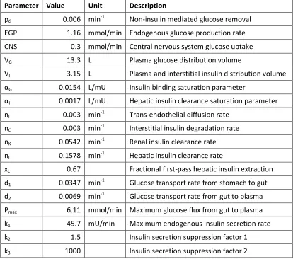
Table 2.1 Parameter values and descriptions for the ICING model.
Parameter Value Unit Description
pG 0.006 min-1 Non-insulin mediated glucose removal
EGP 1.16 mmol/min Endogenous glucose production rate
CNS 0.3 mmol/min Central nervous system glucose uptake VG 13.3 L Plasma glucose distribution volume
VI 3.15 L Plasma and interstitial insulin distribution volume
αG 0.0154 L/mU Insulin binding saturation parameter
αI 0.0017 L/mU Hepatic insulin clearance saturation parameter
nI 0.003 min-1 Trans-endothelial diffusion rate
nC 0.003 min-1 Interstitial insulin degradation rate
nK 0.0542 min-1 Renal insulin clearance rate
nL 0.1578 min-1 Hepatic insulin clearance rate
xL 0.67 Fractional first-pass hepatic insulin extraction
d1 0.0347 min-1 Glucose transport rate from stomach to gut
d2 0.0069 min-1 Glucose transport rate from gut to plasma
Pmax 6.11 mmol/min Maximum glucose flux from gut to plasma
k1 45.7 mU/min Maximum endogenous insulin secretion rate
k2 1.5 Insulin secretion suppression factor 1
k3 1000 Insulin secretion suppression factor 2
2.1
2.2
2.3
2.4
2.5
2.6
11
Table 2.2 Exogenous input variables to the ICING model.
Variable Unit Description
PN(t) mmol/min Intravenous glucose input rate (parenteral nutrition)
D(t) mmol/min Oral glucose input rate (enteral nutrition) uex(t) mU/min intravenous insulin input rate
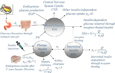
Figure 2.1 shows a schematic diagram of the ICING model. This diagram includes both the glucose-insulin system and the gastric component, which models the movement of glucose from nutrition through the stomach to the gut and subsequent absorption into the glucose compartment. The glucose, plasma insulin and interstitial insulin compartments of the glucose-insulin system are shown as circles, denoted G(t), I(t) and Q(t), respectively. The kinetics, appearance and clearance of insulin and glucose are indicated with solid arrows. The dynamic interaction between interstitial insulin and insulin-mediated glucose uptake, governed by the SI model parameter, is indicated with a dashed arrow.
[image:29.595.97.496.452.704.2]12
In the ICING model, insulin sensitivity, SI, is the critical patient-specific parameter that is fitted hourly to clinical blood glucose measurements using an integral-based fitting method [Hann et al. 2005]. The identification of SI relies not only on measured BG concentrations, but also the interstitial insulin concentration and total glucose flux through the compartment, both of which cannot be measured directly in clinical real-time. These other factors are primarily influenced by insulin kinetics, defined by nI and nC, and the modelled endogenous insulin (Uen) and glucose (EGP) appearance rates. However, with limited clinical data available, only one model parameter, SI can be uniquely identified [Docherty et al. 2011]. Hence, these other parameters must be treated as population constants or modelled independently.
Thus, the task of reducing intrinsic SI variability boils down to using the best data available to determine or model these particular parameters as accurately as possible for a fairly broad, critically ill population. A major goal of this thesis is to explore the impact of several specific model parameters and incorporate new physiological data to improve clinical performance and physiological relevance:
Chapter 3 uses recently obtained clinical data to develop a more accurate model of endogenous insulin secretion for critically ill patients. This sub-model is of particular importance as endogenous insulin can make up a large part of the total insulin appearance rate and consequently has a significant impact on SI.
Chapter 4 investigates the kinetic parameters nI and nC, which define the diffusion of insulin between the plasma and interstitium and cell-receptor binding and clearance. The interactions between these two parameters determine the maximum interstitial insulin concentrations and thus insulin-mediated glucose disposal.
13
appearance, particularly during the early part of a patient’s ICU stay. Thus, as with insulin secretion, EGP can have a significant impact on SI.
2.2 Role of SI in model-based control
The model-based glycaemic control approach used in this thesis is known as STAR (Stochastic, TARgeted) [Evans et al. 2012; Evans et al. 2011]. The STAR approach relies on the physiological model (Equations 2.1- 2.7) and one or more stochastic models of SI that describe the probability density of SI for the forthcoming hour, given the value identified over the previous hour. These stochastic models of SI enable BG concentrations to be forecast one or more hours ahead with associated confidence levels, given known or proposed insulin and nutritional inputs. This process is illustrated schematically in Figure 2.2.
Figure 2.2. BG forecasting based on a stochastic model of SI.
The generation and validation of these stochastic models are described in detail by Lin [2007]. Briefly, existing data from critically ill patients are used to identify
SI profiles with the ICING model. The SI profiles are broken down into paired (SIn, SIn+1) data points and kernel density estimation methods used to create a smooth, continuous model surface that reflects the sample data pattern. Specifically, SIn+1 ~ F(SIn) and thus, for any identified value of SIn,, the stochastic model provides a continuous, empirical estimate of the probability function of
SIn+1, for the subsequent hour. Experience has shown that a minimum of approximately 1300 hours of data is required to generate reliable stochastic models.
Insulin sensitivity
Blood glucose tnow
Stochastic model shows the bounds (5th– 95thpercentile)
for insulin sensitivity variation over next 1-3 hours from the initially identified level
For a given feed+insulin intevention an output BG distribution can be forecast using the model
tnow+(1-3)hr
95th
75th
50th
25th
5th
5th
25th
50th
75th
14
The ability to forecast BG concentrations with associated confidence levels enables the STAR control algorithm to optimise insulin and nutrition inputs, while keeping the risk of hypoglycaemia below a clinically specified limit (typically 5%). The STAR approach explicitly targets the 5th and 95th percentile forecast BG outcomes (Figure 2.2.) to the clinically selected target BG range. Hence, STAR aims to maximise the likelihood that the next BG measurement will be in the desired target range, given constraints on the risk of hypoglycaemia and nutrition and insulin administration.
The stochastic method captures behaviours of the cohort used to generate the models. However any particular patient is not guaranteed to follow cohort-defined behaviour, and can be influenced by external factors such as individual disease state and therapy. The task of reducing the impact of extrinsic SI
15
Chapter 3.
Endogenous Insulin Secretion Model
This section investigates intrinsic SI variability, resulting from the unmodelled variability of other parameters within the physiological model. The endogenous insulin secretion model is of particular importance as endogenous insulin can make up a large part of the total insulin appearance rate. Thus, endogenous insulin has a significant impact on identified values of SI and consequently, intrinsic SI variability.
3.1 Introduction
Correctly modelling endogenous (pancreatic) insulin secretion is important to the overall accuracy of any glucose-insulin system model. In the absence of exogenous insulin or with low-doses, endogenous secretion is responsible for a significant percentage of insulin-mediated glucose disposal. Therefore, it has a significant impact on the identified SI parameter, particularly in these situations. Hence, reducing error in the insulin secretion model can reduce intrinsic SI
variability and thus increase the accuracy and utility of the parameter for glycaemic control.
A number of studies have established models of endogenous insulin secretion as a function of blood glucose level and its derivative, almost exclusively in healthy and diabetic individuals [Camastra et al. 2005; Ferrannini et al. 2005; Mari et al. 2002a; Mari et al. 2002b]. These models primarily focus on the endogenous response to glycaemic change resulting from meals. However, during critical illness, endogenous secretion may be enhanced, [Black et al. 1982; Watters et al. 1997] possibly due to stress hyperglycaemia. Equally, it may be suppressed by counter-regulatory hormones such as adrenaline, cortisol and glucagon [Bessey & Lowe 1993; Deibert & DeFronzo 1980; Gelfand et al. 1984]. Hence, healthy and diabetic insulin secretion models may not be appropriate to critically ill patients.
16
clinical trial studying sepsis in the Christchurch Hospital ICU, 19 patients had blood samples taken to determine pre-hepatic endogenous insulin secretion. From this data, a model of insulin secretion as a function blood glucose could be identified.
3.2 Subjects and Methods
3.2.1 Patients and samples
19 patients from the Christchurch Hospital ICU enrolled in a prospective clinical trial studying sepsis each had an additional two sets of blood samples assayed for insulin and C-peptide. Patients were included in the study if they met all of the following criteria:
Age ≥ 16 years.
Expected survival ≥ 72 hours.
Expected ICU length of stay ≥ 48 hours.
Entry to the SPRINT TGC protocol (2 sequential BG measurements ≥ 8 mmol/l).
Suspected sepsis or SIRS score ≥ 3.
Patients with suspected sepsis received treatment for sepsis with antibiotics. No diagnosed Type I diabetic patients were included. This study was approved by the Upper South Regional Ethics Committee, New Zealand.
Table 3.1 Summary of patient characteristics. Data are shown as median [IQR] where appropriate.
N 19
Age (years) 68 [57-75]
Gender (M/F) 10/9
APACHE II score 22.0 [18.3-26.8]
Confirmed sepsis 79%
Hospital mortality (L/D) 13/6
Diagnosed T2DM 3
17
Two further patients each only had one set of blood samples assayed as one was discharged from the ICU within 48 hours and the other did not meet the criteria for the second set to be taken.
Table 3.2 Summary of patient diagnoses.
APACHE III diagnoses Number
Non-operative
Respiratory 9
Gastrointestinal 1
Neurological 2
Sepsis 4
Operative Gastrointestinal 2
Trauma 1
Each patient had two sets of blood samples taken, where each set consisted of 4 separate samples. The first set of samples was taken at the commencement of the SPRINT TGC protocol. The second set was taken when the patient consistently met less than 2 of the SIRS criteria (Systemic Inflammatory Response Syndrome) [1992].
The first sample of each set was taken immediately prior to bolus delivery of insulin as required by SPRINT (t = -1 min). The remaining three samples were taken at t = 10, 40 and 60 min. Plasma was separated from the blood samples and frozen for subsequent analysis. The testing laboratory reported that one sample (out of 143) was extremely haemolysed, to the extent that it may have lowered the measured C-peptide concentration and was thus excluded from the analysis.
18
Insulin and C-peptide concentrations were determined using immunometric assays (Elecsys 2010, Roche Diagnostics, Germany). Blood glucose levels were measured with a bedside glucometer (Super-Glucocard II, Arkray Inc., Japan). The reported coefficients of variation (CVA) for the insulin and C-peptide assays were 3.8% and 4.5% respectively [Roche 2004,2005]. Measurement error for the BG sensors was typically around 10% [Arkray 2007] (Chapter 9).
3.2.2 Analysis methods
Endogenous insulin secretion (Uen) can be determined from a series of plasma C-peptide measurements. C-peptide is produced by the pancreatic β-cells as a by-product of splitting insulin from its precursor, proinsulin, and is secreted in equimolar ratio with insulin [Rubenstein et al. 1969]. Unlike insulin, C-peptide is cleared almost entirely by the kidneys, making it a much more reliable marker of endogenous secretion than plasma insulin concentrations. Therefore, models independently linking C-peptide kinetics and insulin kinetics can be used to determine and capture pre-hepatic insulin secretion [Polonsky et al. 1986; Van Cauter et al. 1992].
The pharmacokinetic model and population kinetic parameters reported by Van Cauter et al. [1992] were used to deconvolve insulin secretion rates from measured C-peptide data. Age-based kinetic parameters were used for non-diabetic patients, while the population parameters reported for T2DM subjects were used for patient with diagnosed or suspected type II diabetes.
19
Model fitting was performed by minimising the sum of the geometric means of the squared deviations in each dimension. This method allows for uncertainty in both the dependent and independent variables, while maintaining scale invariance [Draper & Yang 1997; Tofallis 2002]. Goodness of fit was assessed using the coefficient of determination, R2, calculated for the constrained model.
3.3 Results and Discussion
3.3.1 Calculated endogenous secretion rates
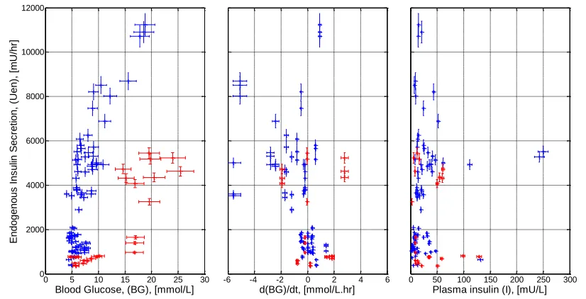
Figure 3.1 shows calculated pre-hepatic insulin secretion plotted against blood glucose, its derivative and plasma insulin. The distinct group at the lower right of the left panel of Figure 3.1 (shown in red) consists of the three diagnosed type II diabetic patients and two others with a significantly impaired insulin response to hyperglycaemia. The clear separation between these patients and the remainder of the cohort suggests two separate models for insulin secretion; one for non-diabetic patients and one for diagnosed or suspected type II non-diabetic patients.
Figure 3.1 Pre-hepatic insulin secretion plotted against each of the measured variables. Data indicating patients with an impaired insulin response to hyperglycaemia are shown in red.
0 5 10 15 20 25 30 0 2000 4000 6000 8000 10000 12000
Blood Glucose, (BG), [mmol/L]
E n d o g e n o u s I n s u lin S e c re ti o n , (Uen ), [m U/h r]
-6 -4 -2 0 2 4 6
d(BG)/dt, [mmol/L.hr]
0 50 100 150 200 250 300
[image:37.595.93.506.413.624.2]20 3.3.2 Secretion rate bounds
It is likely that there is a physiological upper limit on pancreatic secretion rate. A non-zero minimum secretion rate is also required by the ICING model to prevent large insulin sensitivity changes when exogenous insulin is started or stopped. With little or no exogenous insulin and low pancreatic secretion rates (<500 mU/hr) the concentration of the remote insulin compartment (Q) approaches zero. Hence, mathematically, SI must be very large to maintain the observed glucose flux.
In a study of the potentiating effects of glucagon-like-peptide-1 (GLP-1) on insulin secretion, Kjems et al. [2003] achieved some very secretion high rates that suggest a reasonable physiological upper bound. The study involved stepped glucose infusions at 4 rates of GLP-1 infusion (0, 0.5, 1.0 & 2.0 pmol/kg.min) given to type II diabetic patients and healthy controls. Insulin secretion rates were deconvolved using the method and population parameters of Van Cauter et al [1992]. Figure 3.2, reproduced from Kjems et al. [2003], shows the calculated insulin secretion rates (ISR) as a function of BG for healthy subjects receiving the maximum GLP-1 infusion, when insulin secretion is maximally stimulated. Estimating the maximum achieved at 20 pmol/kg.min corresponds to 16000 mU/hr for an 80kg subject.
Figure 3.2 Mean dose-response relationship between plasma glucose and pre-hepatic insulin secretion rates of healthy subjects during graded glucose infusion with a GLP-1 dose of 2.0 pmol/kg.min. [Kjems et al. 2003].
21
rate of 53 pmol/min.m2 for lean, non-diabetic subjects. Assuming a body surface area (BSA) of 1.8m2, this value corresponds to a rate of 954 mU/hr. The values reported by Kjems et al. [2003] and Ferrannini et al. [2005] suggest that upper and lower bounds on pre-hepatic insulin secretion rates of 16000 mU/hr and 1000 mU/hr would be appropriate.
3.3.3 Model fitting
As in previous studies [Camastra et al. 2005; Ferrannini et al. 2005; Mari et al. 2002a; Mari et al. 2002b], models of the form shown in Equation 3.1 were fitted to the data. Where xj denotes the independent variables (BG, dBG/dt, plasma
insulin) and c is a bias constant.
3.1
Model fitting was performed by minimising the sum of the geometric means of the squared deviations in each dimension [Tofallis 2002]. Endogenous secretion was constrained between upper and lower bounds of 16000 mU/hr and 1000 mU/hr. The resulting model coefficients (aj) and goodness of fit values are shown in Table 3.3.
Table 3.3 Coefficients for endogenous insulin secretion models fitted with 1, 2 and 3 independent variables (dimensions).
Model
Coefficients
Goodness of fit
(R2) Constant
c
[mU/hr]
Blood glucose
a1
[mU.l/mmol.hr]
BG derivative
a2
[mU.l/mmol]
Plasma insulin
a3
[l/hr]
N
o
n
-d
iab
et
ic 1-dim. -2996 893 0.61
2-dim. -2573 760 -773 0.59
3-dim. -2811 848 -931 -23 0.41
T2
D
M
1-dim. -1644 296 0.69
2-dim. -1466 302 -586 0.69
22
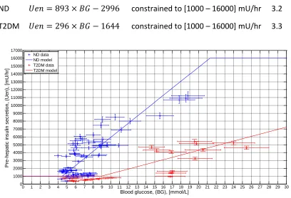
The best model for insulin secretion, in terms of both fit to data and simplicity is the 1-dimensional model based on blood glucose level alone. Figure 3.3 shows the data and both non-diabetic (blue) and T2DM models (red). Equations 3.2 and 3.3 describe the non-diabetic and T2DM models, respectively.
Figure 3.3 Pre-hepatic insulin secretion data and 1-dimensional model fits. Non-diabetic data and model shown in blue (R2 = 0.61); T2DM data and model shown in red (R2 = 0.69).
Two points of particular note regarding the model fit are the variability in secretion rate and the number of points below the lower bound. There is considerable variability in secretion rates for any given blood glucose level, particularly in the range 6-10mmol/l. For example, blood glucose measurements in the range 6.5-7.0 mmol/l are associated with secretion rates between 1319-6076 mU/hr, a 4.5-fold range. In addition, individual patients show a range of secretion rates spanning up to 2385 mU/hr within a 60-minute period. There are numerous data points (23%) below the minimum secretion level of 1000 mU/hr including one identified at –52.5 mU/hr (not shown).
0 1 2 3 4 5 6 7 8 9 10 11 12 13 14 15 16 17 18 19 20 21 22 23 24 25 26 27 28 29 30 0 1000 2000 3000 4000 5000 6000 7000 8000 9000 10000 11000 12000 13000 14000 15000 16000 17000
Blood glucose, (BG), [mmol/L]
P re -h e p a ti c i n s u lin s e c re ti o n , (Uen ), [m U/h r] ND data ND model T2DM data T2DM model
[image:40.595.93.501.177.455.2]23
Both the inter- and intra patient variability and the number of points below the lower bound are likely a result of using population kinetic parameters for the C-peptide model. The study by Van Cauter et al. [1992] shows considerable variation between patients. Coefficients of variation for the kinetic parameters of normal and T2DM subjects were reported in the range 16-36% and the linear regression of long half-life against age had a correlation coefficient, r=0.28. Thus, there was significant variation around the best-fit population parameters.
Physiologically, the cause of the secretion rates below the lower bound could also be due to diminished secretion capacity. Of the 24 data points (23%) below 1000 mU/hr, 13 were from the five type II diabetic individuals or suspected, undiagnosed individuals.
3.3.4 Model validation
To validate the secretion model, comparisons were made to published data. There is very little data available in the literature concerning insulin secretion rates in critically ill patients. Most studies tend to focus on healthy subjects and those with diabetes. Table 3.4 presents the results of a number of published studies in which insulin secretion profiles have been related to blood glucose levels. All these studies used the method and kinetic parameters of Van Cauter et al. [1992] to calculate insulin secretion rates from plasma C-peptide concentrations.
24
Table 3.4 Glucose coefficient data from the literature. Results have been converted to the units of measurement used in this study where necessary. Assumptions used for these conversions were: w = 80 kg; BSAlean = 1.8 m2; BSAobese/T2DM = 2.1 m2.
Study Cohort
Glucose coefficient
a1
[mU.l /mmol.hr]
Ferrannini et al. [2005]
Lean normal glucose tolerance 2646 Obese normal glucose tolerance 1932 Impaired glucose tolerance 1155
T2DM 294
Mari et al. [2002b]
Control 2664
T2DM 1113
Mari et al. [2002a]
Healthy 24 hr meal test (5-7 mmol/l) 2196 Healthy 2 hr protocol (5-7 mmol/l) 2592 Healthy OGTT (5-7 mmol/l) 2754 Camastra et al.
[2005]
Healthy controls 1290
20 Obese Non-Diabetic 1860
Kjems et al. [2003]
Healthy saline infusion 480
T2DM saline infusion 160
Healthy GLP-1 max. infusion rate 5360 T2DM GLP-1 max. infusion rate 1040 Jones et al.
[1997]
Non-diabetic insulin sensitive 485 Non-diabetic insulin resistant 664 Byrne et al.
[1995]
No MODY1 mutation baseline 761 No MODY1 mutation glucose-primed 1400
Chang et al. [2003]
T2DM with NN2211 (GLP-1 derivative) 1008
T2DM with Placebo 432
Controls 1152
3.3.5 Limitations
25
Linear interpolation of BG values resulted in a single value for dBG/dt for each set of measurements, possibly compromising the utility of this specific parameter as an independent variable in the model. However, the utility of dBG/dt is questionable in a critical care model where BG is kept relatively constant with a glycaemic control protocol and patients are fed by constant infusion (enterally or parenterally). This term has more relevance in secretion models in response to a bolus meal or glucose challenge as seen in studies on type II diabetic subjects [Ferrannini et al. 2005; Mari et al. 2002a; Mari et al. 2002b], where the dBG/dt term is only used when the change in BG is positive.
Insulin secretion rates calculated in this study relied on the population kinetic parameters reported by Van Cauter et al. [1992] for healthy and diabetic subjects. Use of these values assumed that renal uptake of C-peptide in critically ill patients was not significantly different to healthy subjects. No published studies were found reporting renal C-peptide metabolism in critically ill patients. Hence, short of repeating the work of Van Cauter in a critically ill population, the values used provided the best available estimates of the transport parameters, and have been used by others in this setting [Hovorka et al. 2008].
In the ICU, renal dysfunction is relatively common. Changes to the renal metabolism of C-peptide resulting from kidney dysfunction would cause errors in the calculated insulin secretion rates from this study as the deconvolution depends upon population estimates of the renal C-peptide clearance rate. In this study one patient was diagnosed with renal failure, however their circulating C-peptide levels and resulting insulin secretion rates were not substantially different from the other patients, so they were not excluded from the analysis.
3.3.6 Impact on SI
26
the range 4.0-7.0 mmol/L, the model developed in this analysis would result in secretion rates of 1000-3300 mU/hr, which are comparable to 2800 mU/hr and thus unlikely to have a significant impact on SI. At higher BG levels, the secretion rates could be significantly higher and thus, the identified value of SI would be lower. Hence, the impact of the proposed models on SI is dependent upon the specific BG concentration and diabetic status of the patient.
The models proposed in this study better capture the variability of insulin secretion, evident in Figure 3.3, than the current, relatively constant, secretion model. However, considerably variability in secretion rate, not accounted for by BG concentration, still remains. Thus, while these new models represent a significant improvement over the current model, and will reduce unwanted intrinsic variability from SI, some variability will persist and affect the identified values of SI.
3.4 Summary
The results of this study show that a simple constrained linear function of blood glucose provided the best model of pre-hepatic insulin secretion in critically ill patients. Separate models were identified for non-diabetic patients and diagnosed or suspected type II diabetic patients with R2 = 0.61 and 0.69 respectively. The glucose coefficients of 893 and 296 mU.l/mmol.hr identified for non-diabetic and diabetic patients were comparable to data published in a number of other studies.
27
Chapter 4.
Interstitial Insulin Kinetics
Like endogenous insulin secretion, insulin kinetics are a potential source of unwanted variability in model-based estimations of SI. The parameters describing insulin clearance and transport vary between individuals and over time. However, unlike insulin secretion, identifying the transport parameter values directly is difficult, if not impossible, and there are as yet no models relating them to readily measurable clinical variables. Population constants based on data from healthy individuals are therefore the best available estimates, for example [Sherwin et al. 1974; Van Cauter et al. 1992]. Nonetheless, these constant parameters need to be optimised to the target population to ensure maximum accuracy and utility of the insulin sensitivity parameter.
4.1 Introduction
Insulin-mediated glucose uptake primarily occurs from the interstitial fluid. Insulin from plasma is transported to the interstitial fluid surrounding tissue cells where it binds to cell-wall receptors, activating glucose uptake [Jefferson & Cherrington 2001]. Hence, correctly modelling interstitial insulin kinetics is important to reducing unwanted intrinsic variability in model-based SI.
28
The parameter identification conducted by Lin et al. [2011] utilised a grid-search to minimise the fitting and prediction errors of the model over 42941 hours of data from 173 critically ill patients. Although providing the mathematically optimal parameter values for that particular cohort, the grid-search method did not necessarily enhance the physiological foundations of the model. In particular, the optimal parameters were centred in parameter spaces with consistently low errors so that a wide range of parameter values was admissible for very limited difference in model performance.
This study extended the fitting and prediction error grid-search identification of the interstitial insulin kinetic parameters of Lin et al. [2011] to two further, independent, critically ill cohorts. Additionally, data from published microdialysis studies was used to directly determine the kinetic parameters from physiological measurements. These better data are used to more accurately justify and validate the parameters chosen.
4.2 Subjects and Methods
This investigation of interstitial insulin kinetic parameters was conducted in two stages. Initially, the grid-search of Lin et al. [2011] was repeated on two independent cohorts to confirm a suitable domain of values consistent with acceptable model performance. This step was followed by the analysis of data from 6 published studies (12 data sets) that used microdialysis to assay interstitial insulin levels simultaneously with plasma insulin levels, enabling direct determination of the kinetic parameters.
4.2.1 Patients