Dynamic Problems of the Planets and Asteroids, and Their Discussion

Dynamic Problems of the Planets and Asteroids, and

Their Discussion

Joseph J. Smulsky1*_{, Yaroslav J. Smulsky}2

1_{Institute of the Earth’s Cryosphere, Siberian Branch of Russian Academy of Sciences, Tyumen, Russia} 2_{Institute of Thermophysics of Russian Academy of Sciences, Siberian Branch, Novosibirsk, Russia}

Email: *_{jsmulsky@mail.ru, ysmulskii@mail.ru}

Received February 9, 2012; revised March 15, 2012; accepted April 18, 2012

ABSTRACT

The problems of dynamics of celestial bodies are considered which in the literature are explained by instability and randomness of movements. The dynamics of planets orbits on an interval 100 million years was investigated by new numerical method and its stability is established. The same method is used for computing movements of two asteroids Apophis and 1950 DA. The evolution of their movement on an interval of 1000 is investigated. The moments of their closest passages at the Earth are defined. The different ways of transformation of asteroids trajectories into orbits of the Earth’s satellites are considered. The problems of interest are discussed from the different points of view.

Keywords: Dynamics; Planets; Asteroids; Satellites; Stability; Discussion

1. Introduction

In the last decades a number of problems associated with the precision of calculating movements have accumu- lated in the celestial and the space dynamics. It was found that there were discrepancies between the calcu- lated and the observed movements. These differences were the cause of the conclusions about chaotic move- ments and the impossibility of accurately calculating them. In addition to Newton’s gravitational forces were introduced weaker forces of other nature, as well as new substances “dark energy” and “dark matter”. In this paper we consider the problems that are associated only with the dynamics of the two groups of celestial objects: With planets and asteroids.

In the study of the evolution of the Solar system over geological time scales the number of researchers has come to the conclusion that there are the instability of the planetary orbits and chaotic motions in the Solar system. For example, in paper [1], it is noted that the eccentricity of the orbit of Mars can be greater than 0.2, and chaotic diffusion of Mercury is so great that his eccentricity can potentially reach values close to 1 and the planet could be thrown out of the Solar system. Already at the time intervals of 10 Myr (million years) there is the weak di- vergence of the Earth’s orbit [2], which, according to these authors, is caused by multiple resonances in the Solar system. Due to them the movement of Solar system is chaotic. Therefore the motion of the Earth [2] and

Mars [3] with an acceptable accuracy cannot be calcu- lated for a time greater than 20 Myr.

The same problems of dynamics are occurred in the study of motion of asteroids. Unlike the planets, their movement is considered on a smaller time intervals. However, the higher accuracy of determination of their movement is required. In connection with the urgency of the tasks of asteroids motion the problems of their dy- namics is considered in more detail.

Over the past decade, the asteroids of prime interest have been two asteroids, Apophis and 1950 DA, the first predicted to approach the Earth in 2029, and the second, in 2880. Reported calculations revealed some probability of an impact of the asteroids on the Earth. Yet, by the end of the decade refined orbital-element values of the asteroids were obtained, and more precise algorithms for calculating the interactions among solar-system bodies were developed. Following this, in the present paper we consider the motion evolution of both asteroids. In addi- tion, we discuss available possibilities for making the asteroids into the Earth-bound satellites. Initially, the analysis is applied to Apophis and, then, numerical data for 1950 DA obtained by the same method will be pre- sented.

The background behind the problem we treat in the present study was recently outlined in [4]. On June 19-20, 2004, asteroid Apophis was discovered by astronomers at the Kitt Peak Observatory [5], and on December 20, 2004 this asteroid was observed for the second time by astronomers from the Siding Spring Survey Observato-

ry [6]. Since then, the new asteroid has command inter- national attention. First gained data on identification of Apophis’ orbital elements were employed to predict the Apophis path. Following the first estimates, it was re- ported in [7] that on April 13, 2029 Apophis will ap- proach the Earth center to a minimum distance of 38,000 km. As a result of the Earth gravity, the Apophis orbit will alter appreciably. Unfortunately, presently available methods for predicting the travel path of extraterrestrial objects lack sufficient accuracy, and some authors have therefore delivered an opinion that the Apophis trajectory will for long remain unknown, indeterministic, and even chaotic (see [4,7,8]). Different statistical predictions points to some probability of Apophis’ collision with the Earth on April 13, 2036. It is this aspect, the impact risk, which has attracted primary attention of workers dealing with the problem.

Rykhlova et al. [7] have attempted an investigation into the possibility of an event that the Apophis will closely approach the Earth. They also tried to evaluate possible threats stemming from this event. Various means to resist the fall of the asteroid onto Earth were put for- ward, and proposals for tracking Apophis missions, made. Finally, the need for prognostication studies of the Apo- phis path accurate to a one-kilometer distance for a pe- riod till 2029 was pointed out.

Many points concerning the prospects for tracking the Apophis motion with ground- and space-based observing means were discussed in [4,7-9]. Since the orbits of the asteroid and Earth pass close to each other, then over a considerable portion of the Apophis orbit the asteroid disc will only be partially shined or even hidden from view. That is why it seems highly desirable to identify those periods during which the asteroid will appear ac- cessible for observations with ground means. In using space-based observation means, a most efficient orbital al- location of such means needs to be identified.

Prediction of an asteroid motion presents a most chal- lenging problem in astrodynamics. In paper [10], the differential equations for the perturbed motion of the asteroid were integrated by the Everhart method [11]; in those calculations, for the coordinates of perturbing bo- dies were used the JPL planetary ephemeris DE403 and DE405 issued by the Jet Propulsion Laboratory, USA. Sufficient attention was paid to resonance phenomena that might cause the hypothetical 2036 Earth impact.

Bykova and Galushina [12,13] used 933 observations to improve the identification accuracy for initial Apophis orbital parameters. Yet, the routine analysis has showed that, as a result of the pass of the asteroid through several resonances with Earth and Mars, the motion of the aste- roid will probably become chaotic. With the aim to eva- luate the probability of an event that Apophis will impact the Earth in 2036, Bykova et al. [12] have made about 10

thousand variations of initial conditions, 13 of which proved to inflict a fall of Apophis onto Earth.

Smirnov [14] has attempted a test of various integra- tion methods for evaluating their capabilities in predict-ing the motion of an asteroid that might impact the Earth. The Everhart method, the Runge-Kutta method of fourth order, the Yoshida methods of sixth and eighth orders, the Hermit method of fourth and sixth orders, the Mul- tistep Predictor-Corrector (MS-PC) method of sixth and eighth orders, and the Parker-Sochacki method were analyzed. The Everhart and MS-PC methods proved to be less appropriate than the other methods. For example, at close Apophis-to-Earth distances Smirnov [14] used, instead of the Everhart method, the Runge-Kutta method. He came to the fact that, in the problems with singular points, finite-difference methods normally fail to accu-rately approximate higher-order derivatives. This conclu-sion is quite significant since below we will report on an integration method for motion equations free of such deficiencies.

In paper [15] the mathematical problems on asteroid orbit prediction and modification were considered. Pos- sibilities offered by the impact-kinetic and thermonuclear methods in correcting the Apophis trajectory were evalu- ated.

An in-depth study of the asteroid was reported in paper [4]. A chronologically arranged outline of observational history was given, and the trend with progressively re- duced uncertainty region for Apophis’ orbit-element values was traced. Much attention was paid to discussing the orbit prediction accuracy and the bias of various fac- tors affecting this accuracy. The influence of uncertainty in planet coordinates and in the physical characteristics of the asteroid, and also the perturbing action of other asteroids, were analyzed. The effects on integration ac- curacy of digital length, non-spherical shape of Earth and Moon, solar-radiation-induced perturbations, non-uni- form thermal heating, and other factors, were examined.

The equations of perturbed motion of the asteroid were integrated with the help of the Standard Dynamic Model (SDM), with the coordinates of other bodies taken from the JPL planetary ephemeris DE405. It is a well-known fact that the DE405 ephemerid was compiled as an ap- proximation to some hundred thousand observations that were made till 1998. Following the passage to the ephe- meris DE414, that approximates observational data till 2006, the error in predicting the Apophis trajectory on 2036 has decreased by 140,000 km. According to Gior- gini et al. [4], this error proved to be ten times greater than the errors induced by minor perturbations. Note that this result points to the necessity of employing a more accurate method for predicting the asteroid path.

suitable for optical and radar measurements, and also observational programs for oppositions with Earth in 2021 and 2029 and spacecraft missions for 2018 and 2027 were scheduled. Future advances in error minimi- zation for asteroid trajectory due to the above activities were evaluated.

It should be noted that the ephemerides generated as an approximation to observational data enable rather ac- curate determination of a body’s coordinates in space within the approximation time interval. The prediction accuracy for the coordinates on a moment remote from this interval worsens, the worsening being the greater the more the moment is distant from the approximation in-terval. Therefore, the observations and the missions sche- duled in paper [4] will be used in refining future ephe- merides.

In view of the afore-said, in calculating the Apophis trajectory the equation of perturbed motion were inte- grated [4,10,15], while the coordinates of other bodies were borrowed from the ephemerid. Difference integra- tion methods were employed, which for closely spaced bodies yield considerable inaccuracies in calculating higher-order derivatives. Addition of minor interactions to the basic Newtonian gravitational action complicates the problem and enlarges the uncertainty region in pre- dicting the asteroid trajectory. Many of the weak interac- tions lack sufficient quantitative substantiation. More- over, the physical characteristics of the asteroid and the interaction constants are known to some accuracy. That is why in making allowance for minor interactions expert judgments were used. And, which is most significant, the error in solving the problem on asteroid motion with Newtonian interaction is several orders greater than the corrections due to weak additional interactions.

The researches, for example, Bykova and Galushina [12,13] apply a technique in Giorgini et al. 2008 to study of influence of the initial conditions on probability of collision Apophis with Earth. The initial conditions for asteroid are defined from elements of its orbit, which are known with some uncertainty. For example, eccentricity value e = en ± σe, where en is nominal value of eccentric-ity, and σe is root-mean-square deviation at processing of several hundred observation of asteroid. The collision parameters are searched in the field of possible motions of asteroid, for example for eccentricity, 3σe, the initial conditions are calculated in area e = en ± σe. From this area the 10 thousand, and in some works, the 100 thou- sand sets of the initial conditions are chosen by an acci- dental manner, i.e. instead of one asteroid it is consid- ered movement 10 or 100 thousand asteroids. Some of them can come in collision with Earth. The probability of collision asteroid with the Earth is defined by their amount.

Such statistical direction is incorrect. If many mea-

surement data for a parameter are available, then the nominal value of the parameter, say, eccentricity en, pre- sents a most reliable value for it. That is why a trajectory calculated from nominal initial conditions can be re- garded as a most reliable trajectory. A trajectory calcu- lated with a small deviation from the nominal initial con- ditions is a less probable trajectory, whereas the prob- ability of a trajectory calculated from the parameters taken at the boundary of the probability region (i.e. from

e = en ± e) tends to zero. Next, a trajectory with initial

conditions determined using parameter values trice greater than the probable deviations (i.e. e = en ± 3e) has

an even lower, negative, probability. Since initial condi-tions are defined by six orbital elements, then simulta-neous realization of extreme (boundary) values (± 3) for all elements is even a less probable event, i.e. the prob-ability becomes of smaller zero.

That is why it seems that a reasonable strategy could consist in examining the effect due to initial conditions using such datasets that were obtained as a result of suc- cessive accumulation of observation data. Provided that the difference between the asteroid motions in the last two datasets is insignificant over some interval before some date, it can be concluded that until this date the asteroid motion with the initial conditions was deter- mined quite reliably.

As it was shown in paper [4], some additional active- ties are required, aimed at further refinement of Apophis’ trajectory. In this connection, more accurate determina- tion of Apophis’ trajectory is of obvious interest since, following such a determination, the range of possible al- ternatives would diminish.

For integration of differential motion equations of so- lar-system bodies over an extended time interval, a pro- gram Galactica was developed [16-19]. In this program, only the Newtonian gravity force was taken into account, and no differences for calculating derivatives were used. In the problems for the compound model of Earth rota- tion [20] and for the gravity maneuver near Venus [21], motion equations with small body-to-body distances, the order of planet radius, were integrated. Following the solution of those problems and subsequent numerous checks of numerical data, we have established that, with the program Galactica, we were able to rather accurately predict the Apophis motion over its travel path prior to and after the approach to the Earth. In view of this, in the present study we have attempted an investigation into orbit evolution of asteroids Apophis and 1950 DA; as a result of this investigation, some fresh prospects toward possible use of these asteroids have opened.

2. Problem Statement

vity, the differential motion equations have the form [16]:

2

2 3

d

, 1, 2, , d

n

i k ik

k i ik m

G i

t  r

 



r r

n (1)

where i is radius-vector of a body with mass i rela-

tively Solar System barycenter; G is gravitational con- stant; is vector and rik is its module; n = 12.

r

r

m

ik i k

As a result of numerical experiments and their analysis we came to a conclusion, that finite-difference methods of integration do not provide necessary accuracy. For the integration of Equation (1) we have developed algorithm and program Galactica. The meaning of function at the following moment of time t = t0+ t is determined with

the help of Taylor series, which, for example, for coor-dinate x looks like:



r r

 

_{ }

0 0

1 1

!

K

k k

k

x x x

k



 



where _x0 k _{is derivative of k order at the initial moment} t0.

The meaning of velocity x is defined by the similar formula, and acceleration x₀ by the Equation (1). Higher derivatives _x0 k _{we are determined analytically}

as a result of differentiation of the Equation (1). The cal- culation algorithm of the sixth order is now used, i.e. with K = 6.

A few words about the method used and the program Galactica. The algorithms of finite-difference methods are derived from the Taylor series (2). In this case the higher derivatives are determined by the difference of the second derivatives at different steps. This leads to errors of integration. There are methods [22,23], in which the derivatives are determined by recurrence formulas. In the program Galactica the derivatives are calculated under the exact analytical formulas, which we have deduced. This provides greater accuracy than other methods.

Besides in the program Galactica there are many other details, which allow to not reducing the achieved in such way accuracy. They were found in the process of creat- ing the program Galactica. During its development more than 10 different ways to control errors has been used. In our book [19] the following checks are made mention of:

1) Checking the stability of the angular momentum M of the Solar System;

2) Checking the magnitude of the momentum Р of the Solar System;

4) Integrating backwards and forwards in time; 5) Integrating into a remote epoch and subsequent re- turn to the initial epoch;

6) Picking persistent changes (orbital major semiaxis, period, or precession axis etc.) and their checking;

7) Checking against test problems with exact analytic- cal solutions, for example, n-axisymmetrical problem

[24];

8) Comparison with observations; 9) Comparison with other reported data.

The high accuracy of the program Galactica is firstly allowed to integrate Equations (1) for the motion of the Solar System for 100 million years [19]. The error was less on some orders in comparison with work [25], in which this problem has been solved for 3 million years by Stórmer method.

The program Galactica allows solving the problem of interaction of any number of bodies, which motion is described by Equations (1). For example, the problem of the evolution of Earth’s rotation axis [20] was solved. In this task, the rotational motion of the Earth’s has been replaced by a compound model of the Earth’s rotation. The compound model of the Sun’s rotation was used in another task [26], in which the influence of the oblate rotating Sun on the motion of planets was established. In all these problems, this method of integration and pro- gram Galactica had no failures and we successfully used them.

As noted above, the methods, which use Standard Dy- namic Model, are approximation of the data of Solar Sys- tem body’s observations. To calculate the future move- ment of the asteroid the bodies’ positions are used out- side the framework of observation. Therefore the calcu- lation error increases with distance in time from the base of observations. The base of observations is not used in program Galactica, so this error is missing in it. A high accuracy of the integration method of Galactica allows for a smaller error compute motion of asteroids in their rapprochement with the celestial bodies.

The free-access Galactica system, user version for per- sonal computer, can be found at:

http://www.ikz.ru/~smulski/GalactcW. The system of Ga- lactica, except the program Galactica, includes several components, which are described in the User’s Guide http://www.ikz.ru/~smulski/GalactcW/GalDiscrE.pdf. The Guide also provides detailed instructions for all stages of solving the problem. After the free-access system is created based on a supercomputer, we will post the in- formation at the above site.

3. The Dynamics of the Planets’ Orbits

Equa-tions (1) were integrated for 11 bodies: 9 planets, the Sun and the Moon. The motion of bodies is considered in barycentric equatorial coordinates. The parameters of the orbits of the planets are defined in the heliocentric coor-dinate system and the orbit of the Moon is in geocentric coordinates.

The main results obtained with the integration step t = 10–4 _{year and the number of double length (17 decimal).}

Checking and clarifying the calculations were performed with a smaller step, as well as with the extended length of the numbers (up to 34 decimal places).

Methods for validation of the solutions and their errors are investigated in [19]. The computed with the help of the program Galactica change of the parameters of the orbit of Mars at time interval of 7 thousand years is shown in Figure 1 points 1. The eccentricity e and peri- helion angle p increase, and the longitude of the as-

cending node Ω decreases in this span of time. The an-

gle of inclination of the Mars orbit i does not change monotonically. In the epoch at T = 1400 years from 30 December 1949, it has a maximum value. The changing these parameters for a century are called secular pertur-bations. In contrast, the semi-major axis a and orbital period P on the average remains unchanged, so the graphs are given their deviations from the mean values. These fluctuations relative to the average am = 2.279 × 1011 _{m and Pm = 1.881 years have a small value. The}

parameters e, i, Ω and p also vary with the same

rela-tive amplitudes as parameters a and P.

In Figure 1 the lines 2 and 3 show the approximation of the observation data. As one can see, the eccentricity e

and the angles i, Ω andp coincide with observations in

the interval 1000 years, i.e. within the validity of ap- proximations by S. Newcomb [27] and J. Simon et al.

[28]. Calculations for the semi-major axis a and the pe- riods P also coincide with the observations and their fluc- tuations comparable in magnitude with the difference between the approximations of different authors. Similar studies of secular changes in orbital parameters are made for other planets. They are also compared with the ap- proximations of the observational data, except for Pluto. Its approximation of the observations is missing.

In Figure 2 there are the variations of the calculated elements of the orbit of Mars in 3 million years into the past. The eccentricity of the orbit e has short-period os- cillations of amplitude 0.019 with the main period equal to Te1 = 95.2 thousand years. It oscillates relatively the

average for 50 million years value of em = 0.066. The longitude of ascending node Ω oscillates with the aver-

age period of ТΩ = 73.1 thousand years around the mean value Ωm = 0.068 radians. The angle of inclination of the

orbital plane to the equatorial plane i fluctuates with the same period Ti = 73.1 thousand years around the mean value іm = 0.405 radians. Longitude of perihelion φр al-

Figure 1. Secular changes of the Mars orbit 1 compared with approximated observations by Newcomb [27] and Simon et al. [28], 2 and 3, respectively: Eccentricity e; in-clination i to equator plane for epoch J2000.0; longitude of ascending node relative to the x axis at J2000.0;

longi-tude of perihelionp;semi-major axis deviation Δa from the average of 7 thousand years, in meters; orbital period de-viation ΔP from average of 7 thousand years, in centuries. Angles are in radians and time Т is in centuries from 30 December 1949; data points spaced at 200 yr.

most linearly increases with time, i.e. the perihelion moves in the direction of circulation of Mars around the Sun, making on the average for a –50 million years, one revolution for the time Tp = 76.8 thousand years. At the same time its motion is uneven. As one can see from the graph, the angular velocity of rotation of the perihelion p fluctuates around the average value of pm = 1687"

(arc-seconds) per century, while at time T = –1.35 mil-lion years, it takes a large negative value, i.e. in this mo-ment there is the return motion of the perihelion with great velocity.

As a result of research for several million years the pe- riods and amplitudes of all fluctuations of the orbits pa- rameters of all planets received. The system of Equation (1) with the help of the program Galactica was integrated for 100 million years in the past and the evolution of the orbits of all planets and the Moon was studied. Figure 3

shows changing parameters of the Mars orbit on an in- terval from –50 million years to –100 million years. The eccentricity e, angles of inclination i, ascending node Ω

monotonically oscillate. The fluctuations have several periods, and duration of most of them is much smaller than the interval in 50 million years. For example, the greatest period eccentricity Te2 = 2.31 million years. The

angular velocity p of perihelion rotation fluctuate

around the average value of pm. In comparison with the

Figure 3. The evolution of the Mars orbit in the second half of the period of 100 million years: T is the time in millions of years into the past from the epoch 30.12.1949; other no- tations see Figures 1 and 2.

eccentricity e one can see that negative values of p, i.e.

reciprocal motion of the perihelion occurs when the ec- centricity of the orbit is close to zero.

On the interval from 0 to –50 million years the graph- ics have the same form [19], as shown in Figure 3, i.e. the orbit of Mars is both steady and stable and there is no tendency to its change. Similar results were obtained for other planets, i.e. these studies established the stability of the orbits and the Solar system as a whole. The result is important, since in the abovementioned papers [1-3] at solving the problem of other methods after 20 million years, the orbit begins to change, what led to the destruc- tion of the Solar system in the future. Based on these solutions their authors came to the conclusion about the instability of the Solar system and chaotic motions in it.

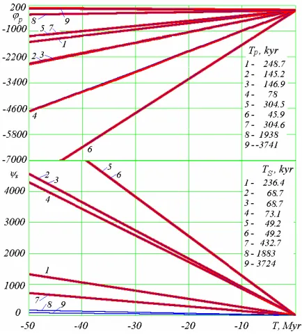
During these researches we have established, that the evolution of the planets orbits is the result of four move- ments: 1) The precession of the orbital axisSaround a fixed in space vector of angular momentum of the Solar system; 2) Nutational oscillations of the orbit axis

M

S; 3) The oscillations of orbit; 4) the rotation of the orbit in its own plane (rotation of the perihelion). The behavior of the perihelion of the orbits of all planets in the span of 50 million years is shown in Figure 4 as a function of angles perihelion φр versus time. The orbits of the eight planets from Mercury to Neptune are orbiting counter- clockwise, i.e. in the direction of orbital motion. The orbit of Pluto, the only one, that rotates clockwise. Two

groups of planets (Venus and Earth, Jupiter and Uranus), as seen from the values of the periods Tp, have almost the same velocity of perihelion rotation. The orbit of Saturn has the highest velocity, and the orbit of Pluto has the smallest one.

should also be emphasized that reported in literature resonances and instabilities appear in the simplified equ- ations of motion when they are solved by approximate analytical methods. These phenomena do not arise at the integrating not simplified Equation (1) by method (2). The precession of the orbit occurs clockwise, i.e.

against the orbital motion of the planets The angle of precession S of the orbit axis is defined in the plane

perpendicular to the vector of the momentum . This plane crosses the equator plane on the line directed at an angle φΩm = 0.068 to the x axis. Precession angle S is

the angle between the line of intersection and the node of the planet orbit. The angle S, as the angle of the peri-

helion φр, varies irregularly, but a large time interval of 50 million years, as shown in Figure 4, these irregular- rities are not visible. As can be seen from the periods of

TS, the orbits axis of Jupiter and Saturn precess with maximum velocity and Pluto—with the lowest one. For the two groups of planets: Venus and Earth, Jupiter and Saturn, the velocity of precession is practically the same.

M

4. Preparation of Initial Data of Asteroids

a, the ecliptic obliquity ie, the ascending node angle , the ascending node-perihelion angle ωe, etc., and aste- roids position elements, such as the mean anomaly M, were borrowed from the JPL Small-Body database 2008 as specified on November 30, 2008. The data, represent- ed to 16 decimal digits, are given in Table 1.

For Apophis in Table 1 the three variants are given. The first variant is now considered. These elements cor- respond to the solution with number JPL sol. 140, which is received Otto Mattic at April 4, 2008. In Table 1 the uncertainties of these data are too given. The relative un- certainty value  is in the range from 2.4 × 10–8 _{to 8 ×}

10–7_{. The same data are in the asteroid database by}

Ed-ward Bowell [29], although these data are represented only to 8 decimal digits, and they differ from the former data in the 7-th digit, i.e., within value . Giorgini et al. [4] used the orbital elements of Apophis on epoch JD = 2453979.5 (September 01, 2006), which correspond to the solution JPL sol.142. On publicly accessible JPL-system It should be emphasized that the secular changes of

angles of inclination i and ascending node Ω in Figure 1

and their variations, are presented by the graphics in Fig- ures 2 and 3, are due to the precessional and nutational motion of the orbit axisS.

The studies testify that the evolution of the planets or- bits in the investigated range is unchanged and stable. This allows us to conclude that the manifestations of in- stability and chaos in the motion of the planets, as de- scribed by other authors, most likely due to the methods of solution which they have been used. Furthermore, it

Table 1. Three variants of orbital elements of asteroids Apophis on two epochs and 1950 DA on one epoch in the heliocentric ecliptic coordinate system of 2000.0 with JDS = 2451545 (see JPL Small-Body Database [30]).

Apophis 1950 DA

1-st variant November 30, 2008

JD01 = 2454800.5 JPL sol.140

Uncertainties ±

1-st var.

2-nd variant January 04, 2010 JD02 = 2455200.5 JPL sol.144

3-rd variant November 30, 2008

JD01 = 2454800.5 JPL sol.144.

November 30, 2008 JD0 = 2454800.5

JPL sol.51

Units Elements

Magnitude

e 0.1912119299890948 7.6088e–08 0.1912110604804485 0.1912119566344382 0.507531465407232

a 0.9224221637574083 2.3583e–08 0.9224192977379344 0.9224221602386669 1.698749639795436 AU q 0.7460440415606373 8.6487e–08 0.7460425256098334 0.7460440141364661 0.836580745750051 AU ie 3.331425002325445 2.024e–06 3.331517779979046 3.331430909298658 12.18197361251942 deg  204.4451349657969 0.00010721 204.4393039605681 204.4453098275707 356.782588306221 deg

ωe 126.4064496795719 0.00010632 126.4244705298442 126.4062862564680 224.5335527346193 deg

M 254.9635275775066 5.7035e–05 339.9486156711335 254.9635223452623 161.0594270670401 deg

tp _{(2009-Mar-04.41275013)}2454894.912750123770 5.4824e–05 _{(2010-Jan-22.02323966)}2455218.523239657948 _{(2009-Mar-04. 41275429)}2454894.912754286546 _{(2007-Dec-12.0419368531} 2.454438.693685309 JD_d

P 323.5884570441701 _0.89 1.2409e–05 _3.397e–08 323.5869489330219 _0.89 323.5884551925927 _0.89 808.7094041052905 _2.21 D _yr

n 1.112524233059586 4.2665e–08 1.112529418096263 1.112524239425464 0.445153720449539 deg/d

Horizons the solution sol.142 can be prolonged till No-vember 30.0, 2008. In this case it is seen, that difference of orbital elements of the solution 142 from the solution 140 does not exceed 0.5 uncertainties of the orbit ele-ments.

The element values in Table 1 were used to calculate the Cartesian coordinates of Apophis and the Apophis velocity in the barycentric equatorial system by the fol- lowing algorithm (see [19,20,31,32]).

From the Kepler equation sin

E e  EM (3) we calculate the eccentric anomaly E and, then, from E, the true anomaly 0:



 

 

0 2 arctg 1 e 1 e tg 0.5 E

   _    



In subsequent calculations, we used results for the two-body interaction (the Sun and the asteroid) [21,32]. The trajectory equation of the body in a polar coordinate

system with origin at the Sun has the form:





p

R r

  



  (5)

where the polar angle φ, or, in astronomy, the true ano- maly, is reckoned from the perihelion position r = Rp;





1 1 1 e

    is the trajectory parameter; and Rp =





r υ

2 1

a a  a is the perihelion radius. The expressions for the radial and transversal velocities are υt



 



1 1 1 1 ,

r p t p

υ  υ      r υ υ r, (6)

where for φ > πwe haveυr0; r= r/Rp is the dimen-sionless radius, and the velocity at perihelion is



 



p S As

υ  G m m  R_p , (7)

where mS=m11 is the Sun mass (the value of m11 is given

in Table 2), and mAs = m12is the Apophis mass.

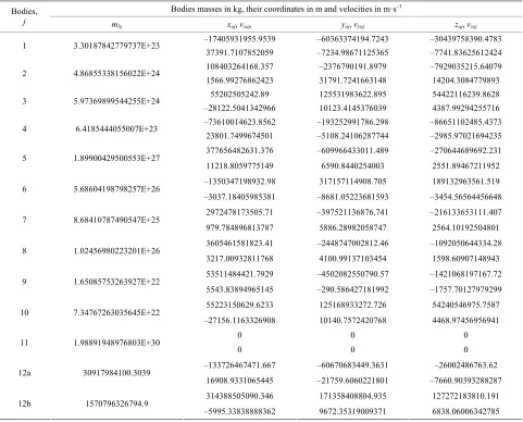
Table 2. The masses mbj of the planets from Mercury to Pluto, the Moon, the Sun (1 - 11) and asteroids: Apophis (12a) and 1950 DA (12b), and the initial condition on epoch JD0 = 2454800.5 (November 30, 2008) in the heliocentric equatorial coor- dinate system on epoch 2000.0 JDS = 2451545. G = 6.67259E–11 m3·s–2·kg–1.

Bodies masses in kg, their coordinates in m and velocities in m·s–1 Bodies,

j _{mbj xaj, vxaj, yaj, vyaj zaj, vzaj}

–17405931955.9539 –60363374194.7243 –30439758390.4783 1 3.30187842779737E+23

37391.7107852059 –7234.98671125365 –7741.83625612424 108403264168.357 –2376790191.8979 –7929035215.64079 2 4.86855338156022E+24

1566.99276862423 31791.7241663148 14204.3084779893 55202505242.89 125531983622.895 54422116239.8628 3 5.97369899544255E+24

–28122.5041342966 10123.4145376039 4387.99294255716 –73610014623.8562 –193252991786.298 –86651102485.4373 4 6.4185444055007E+23

23801.7499674501 –5108.24106287744 –2985.97021694235 377656482631.376 –609966433011.489 –270644689692.231 5 1.89900429500553E+27

11218.8059775149 6590.8440254003 2551.89467211952 –1350347198932.98 317157114908.705 189132963561.519 6 5.68604198798257E+26

–3037.18405985381 –8681.05223681593 –3454.56564456648 2972478173505.71 –397521136876.741 –216133653111.407 7 8.68410787490547E+25

979.784896813787 5886.28982058747 2564.10192504801

3605461581823.41 –2448747002812.46 –1092050644334.28 8 1.02456980223201E+26

3217.00932811768 4100.99137103454 1598.60907148943 53511484421.7929 –4502082550790.57 –1421068197167.72 9 1.65085753263927E+22

5543.83894965145 –290.586427181992 –1757.70127979299

55223150629.6233 125168933272.726 54240546975.7587 10 7.34767263035645E+22

–27156.1163326908 10140.7572420768 4468.97456956941 0 0 0 11 1.98891948976803E+30

0 0 0

–133726467471.667 –60670683449.3631 –26002486763.62 12a 30917984100.3039

16908.9331065445 –21759.6060221801 –7660.90393288287 314388505090.346 171358408804.935 127272183810.191 12b 1570796326794.9

The time during which the body moves along an ellip- tic orbit from the point of perihelion to an orbital position with radius r is given by





















1

1 1 1

3 2 1

2 1

π 2 arcsin 2 1 1

2 1

p r

p

p

p

R r υ

t υ r R υ         _   _     1

  (8)

where r r p

At the initial time t0= 0, which corresponds to epoch

JD0 (see Table 1), the polar radius of the asteroid r0 as

dependent on the initial polar angle, or the true anomaly , can be calculated by Equation (5)The initial radial and initial transversal velocities as functions of r0 can be

found using Equation (6).

υ υ υ

0

is the dimensionless radial velocity.

The Cartesian coordinates and velocities in the orbit plane of the asteroid (the axis xo goes through the perihe- lion) can be calculated by the formulas

0 cos ;0 0 sin

o o

x  r  y  r  (9)

0

0 0

cos sin

sin cos

xo r t

yo r t

υ υ υ

υ υ υ

0

 

 

   

    (10)

The coordinates of the asteroid in the heliocentric ecliptic coordinate system can be calculated as







cos cosΩ sin sinΩ cos

– sin cosΩ cos sinΩ cos ;

e o e e e

o e e e



x x y                i i









cos sinΩ sin cosΩ cos

– sin sinΩ cos cosΩ cos ;

e o e e e

o e e e

y x i

y

 

 

     

     (12)

sin sin cos sin .

e o e e o e

z  x   i y    i (13) The velocity components of the asteroid υ υxe, ye and zein this coordinate system can be calculated by Equa-

tions analogous to (11)-(13).

υ

Since Equation (1) are considered in a motionless equ- atorial coordinate system, then elliptic coordinates (11)- (13) can be transformed into equatorial ones by the Equ- ations

0

0 0

;

cos sin ;

sin sin

a e

a e e

a e e

x x

y y z

z y z

0              (14)

where 0 is the angle between the ecliptic and the equator

in epoch JDS.

The velocity components υ υxe, ye and υze can be

transformed into the equatorial ones υ_xa,υ_ya and _za by Equations analogous to (14). With known heliocentric equatorial coordinates of the Solar system n bodies xai, yai,

zai i = 1, 2, … n, the coordinates of Solar system bary- centre, for example, along axis x will be:

υ

1

n

c i ai Ss

i

X m x M



 

 _



1 n Ss i i M m 





solar system bodies.

Then barycentric equatorial coordinates xi of asteroid and other bodies will be

–

i ai c

x x X .

Other coordinates yi and zi and components of velocity ,

xi yi

υ υ and υ_zi in barycentric equatorial system of co- ordinates are calculated by analogous equations.

In the calculations, six orbital elements from Table 1, namely, e, a ie, ,ωe, and M, were used. Other orbital elements were used for testing the calculated data. The perihelion radius Rp and the aphelion radius Ra =





R a

  were compared to q and Q, respectively. The orbital period was calculated by Equation (8) as twice the time of motion from perihelion to aphelion (r = Ra). The same Equation was used to calculate the mo- ment at which the asteroid passes the perihelion (r = r0).

The calculated values of those quantities were compared to the values of P and tp given in Table 1. The largest relative difference in terms of q and Q was within 1.9 × 10–16_{, and in terms of P and tp, within 8 × 10}–9_.

The coordinates and velocities of the planets and the Moon on epoch JD0 were calculated by the DE406/

LE406 JPL-theory [33,34]. The masses of those bodies were modified by us [18], and the Apophis mass was calculated assuming the asteroid to be a ball of diameter

d = 270 m and density  = 3000 kg/m3_{. The masses of all}

bodies and the initial conditions are given in Table 2. The starting-data preparation and testing algorithm (3)- (14) was embodied as a MathCad worksheet (program AstCoor2.mcd).

5. Apophis’ Encounter with the Planets and

the Moon

In the program Galactica, a possibility to determine the minimum distance Rmin to which the asteroid approaches

a celestial body over a given interval T was provided. Here, we integrated Equation (1) with the initial condi- tions indicated in Table 2. The integration was per- formed on the NKS-160 supercomputer at the Computing Center SB RAS, Novosibirsk. In the program Galactica, an extended digit length (34 decimal digits) was used, and for the time step a value dT = 10–5 _{year was adopted.}

The computations were performed over three time inter- vals, 0 - 100 years (Figure 5(a)), 0 - –100 years (Figure 5(b)), and 0 - 1000 years (Figure 5(c)).

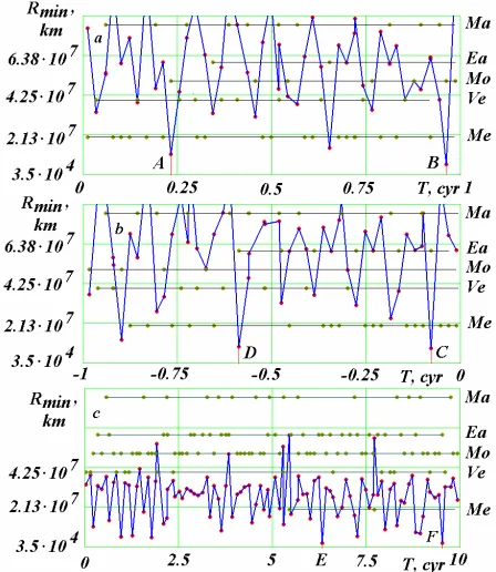
In the graphs of Figure 5 the points connected with the heavy broken line show the minimal distances Rmin to

Figure 5. Apophis’ encounters with celestial bodies during the time T to a minimum distance Rmin, km: Mars (Ma), Earth (Ea), Moon (Mo), Venus (Ve) and Mercury (Me); a, b—

T = 1 year; c—T = 10 years. T,cyr (1 cyr = 100 yr) is the time in Julian centuries from epoch JD0 (November 30, 2008). Calendar dates of approach in points: A—13 April 2029; B—13 April 2067; C—5 September 2037; E—10 Oc-tober 2586.

which, over the time T = 1 year, the asteroid will ap-proach a body denoted by the point in the horizontal line at the same moment. It is seen from Figure 5(a) that, starting from November 30, 2008, over the period of 100 years there will be only one Apophis’ approach to the Earth (point A) at the moment TA = 0.203693547133403

century to a minimum distance RminA = 38907 km. A next

approach (point B) will be to the Earth as well, but at the moment TB = 0.583679164042455 century to a minimum

distance RminB = 622,231 km, which is 16 times greater

than the minimum distance at the first approach. Among all the other bodies, a closest approach with be to the Moon (point D) (see Figure 5(b)) at TD =

–0.106280550824626 century to a minimum distance

RminD = 3,545,163 km.

In the graphs of Figures 5(a) and (b) considered above, the closest approaches of the asteroid to the bodies over time intervals T = 1 year are shown. In integrating Equation (1) over the 1000-year interval (see Figure 5(c)), we considered the closest approaches of the aste- roid to the bodies over time intervals T = 10 years. Over those time intervals, no approaches to Mercury and Mars were identified; in other words, over the 10-year intervals the asteroid closes with other bodies. Like in Figure 5(a), there is an approach to the Earth at the moment TA. A

second closest approach is also an approach to the Earth at the point Е at TE = 5.778503 century to a minimum

distance RminE = 74002.9 km. During the latter approach,

the asteroid will pass the Earth at a minimum distance almost twice that at the moment TA.

With the aim to check the results, Equation (1) were integrated over a period of 100 years with double digit length (17 decimal digits) and the same time step, and also with extended digit length and a time step dT = 10–6

year. The integration accuracy (see Table 3) is defined [19] by the relative change of Mz, the z-projection of the

angular momentum of the whole solar system for the 100-year period. As it is seen from Table 3, the quantity Mz varies from –4.5 × 10–14 to 1.47 × 10–26, i.e., by 12

orders of magnitude. In the last two columns of Table 3, the difference between the moments at which the asteroid most closely approaches the Earth at point A (see Figure 5(a)) and the difference between the approach distances relative to solution 1 are indicated. In solution 2, ob- tained with the short digit length, the approach moment has not changed, whereas the minimum distance has re- duced by 2.7 m. In solution 3, obtained with ten times reduced integration step, the approach moment has changed by –2 × 10–6 _{year, or by –1.052 minutes. This}

change being smaller than the step dT = 1 × 10–5 _{for solu-}

tion 1 and being equal twice the step for solution 3, the value of this change provides a refinement for the ap- proach moment. Here, the refinement for the closest ap- proach distance by –1.487 km is also obtained. On the refined calculations the Apophis approach to the Earth occurs at 21 hours 44 minutes 45 sec on distance of 38905 km. We emphasize here that the graphical data of

Figure 5, a for solutions 1 and 3 are perfectly coincident. The slight differences of solution 2 from solutions 1 and 3 are observed for Т > 0.87 century. Since all test calcu- lations were performed considering the parameters of solution 1, it follows from here that the data that will be presented below are accurate in terms of time within 1’, and in terms of distance, within 1.5 km.

At integration on an interval of 1000 years the relative change of the angular momentum is Mz = 1.45 × 10–20_.

How is seen from the solution 1 of Table 3 this value exceeds Mz at integration on an interval of 100 years in 10 times, i.e. the error at extended length of number is proportional to time. It allows to estimate the error of the

Table 3. Comparison between the data on Apophis’ en- counter with the Earth obtained with different integration accuracies: Lnb is the digit number in decimal digits.

No.

solution Lnb dT, yr Mz TAi–TA1, yr RminA_km i–RminA1, 1 34 1 × 10–5 _{1.47 × 10}–21 _{0 0} 2 17 1 × 10–5 _{–4.5 × 10}–14 _{0 –2.7 × 10}–3

second approach Apophis with the Earth in TE = 578

years by results of integrations on an interval of 100 years of the solution with steps dT = 1 × 10–5 _{years and 1 ×}

10–6 _{years. After 88 years from beginning of integration}

the relative difference of distances between Apophis and Earth has become R88 = 1 × 10–4, that results in an error

in distance of 48.7 km in TE = 578 years.

So, during the forthcoming one-thousand-year period the asteroid Apophis will most closely approach the Earth only. This event will occur at the time TA counted

from epoch JD0. The approach refers to the Julian day

JDA = 2462240.406075 and calendar date April 13, 2029,

21 hour 44'45" GMT. The asteroid will pass at a mini- mum distance of 38905 km from the Earth center, i.e., at a distance of 6.1 of Earth radii. A next approach of Apo- phis to the Earth will be on the 578-th year from epoch

JD0; at that time, the asteroid will pass the Earth at an

almost twice greater distance.

The calculated time at which Apophis will close with the Earth, April 13, 2029, coincides with the approach times that were obtained in other reported studies. For instance, in the recent publication [4] this moment is given accurate to one minute: 21 hour 45' UTC, and the geocentric distance was reported to be in the range from 5.62 to 6.3 Earth radii, the distance of 6.1 Earth radii falling into the latter range. The good agreement between the data obtained by different methods proves the ob- tained data to be quite reliable.

As for the possible approach of Apophis to the Earth in 2036, there will be no such an approach (see Figure 5(a)). A time-closest Apophis’ approach at the point C to a minimum distance of 7.26 million km will be to the Moon, September 5, 2037.

6. Apophis Orbit Evolution

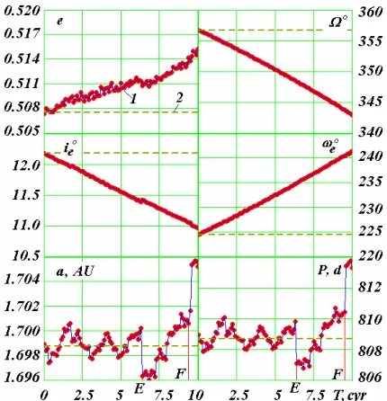
In integrating motion Equation (1) over the interval –1 century ≤T≤ 1 century the coordinates and velocities of the bodies after a lapse of each one year were recorded in a file, so that a total of 200 files for a one-year time in- terval were obtained. Then, the data contained in each file were used to integrate Equation (1) again over a time interval equal to the orbital period of Apophis and, fol- lowing this, the coordinates and velocities of the asteroid, and those of Sun, were also saved in a new file. These data were used in the program DefTra to determine the parameters of Apophis’ orbit relative to the Sun in the equatorial coordinate system. Such calculations were performed hands off for each of the 200 files under the control of the program PaOrb. Afterwards, the angular orbit parameters were recalculated into the ecliptic coor- dinate system (see Figure 6).

As it is seen from Figure 6, the eccentricity е of the Apophis orbit varies non-uniformly. It shows jumps or

Figure 6. Evolution of Apophis’ orbital parameters under the action of the planets, the Moon and the Sun over the time interval −100 years - +100 years from epoch November 30, 2008: 1—as revealed through integration of motion Equation (1); 2—initial values according to Table 1. The angular quantities: , ie, and ωe are given in degrees; the major semi-axis a in AU; and the orbital period P in days.

breaks. A most pronounced break is observed at the mo- ment TA, at which Apophis most closely approaches the

Earth. A second most pronounced break is observed when Apophis approaches the Earth at the moment TB.

The longitude of ascending node  shows less breaks, exhibiting instead rather monotonic a decrease (see Fig-ure 6). Other orbital elements, namely, ie, ωe,a, and P, exhibit pronounced breaks at the moment of Apophis’ closest pass near the Earth (at the moment TA).

The dashed line in Figure 6 indicates the orbit-ele- ment values at the initial time, also indicated in Table 1. As it is seen from the graphs, those values coincide with the values obtained by integration of Equation (1), the relative difference of e, , ie, ωe, a, and P from the initial values at the moment T = 0 (see Table 1) being respec- tively 9.4 × 10–6_{, –1.1 × 10}–6_{, 3.7 × 10}–6_{, –8.5 × 10}–6_{, 1.7 ×}

10–5_{, and 3.1 × 10}–5_{. This coincidence testifies the}

reli-ability of computed data at all calculation stages, includ-ing the determination of initial conditions, integration of equations, determination of orbital parameters, and trans-formations between the different coordinate systems.

those shown in Figure 6. Also, other solution methods for differential equations exist, including those in which expansions with respect to orbital elements or difference quotients are used. As it was already mentioned in Intro- duction, these methods proved to be sensitive to various resonance phenomena and sudden orbit changes ob- served on the approaches between bodies. Equation (1) and method (2) used in the present study are free of such shortcomings. This suggests that the results reported in the present paper will receive no notable corrections in the future.

7. Influence of Initial Conditions

With the purpose of check of influence of the initial con- ditions (IC) on Apophis trajectory the Equation (1) were else integrated on an interval 100 years with two variants of the initial conditions. The second of variant IC is given on January 04, 2010 (see Table 1). They are taken from the JPL Small-Body database [29] and correspond to the solution with number JPL sol.144, received Steven R. Chesley on October 23, 2009. In Figure 7 the results of two solutions with various IC are submitted. The line 1 shows the change in time of distance R between Apo-phis and Earth for 100 years at the first variant IC. As it is seen from the graphs, the distance R changes with os-cillations, thus it is possible to determine two periods: the short period TR1 = 0.87 years and long period TR2. The

amplitude of the short period Ra1 = 29.3 million km, and

long is Ra2 = 117.6 million km. The value of the long

oscillation period up to T ~ 70 years is equal TR20 = 7.8

years, and further it is slightly increased. After ap- proach of April 13, 2029 (point A in Figure 7) the am- plitude of the second oscillations is slightly increased. Both short and the long oscillations are not regular; therefore their average characteristics are above given.

Let’s note also on the second minimal distance of Apophis approach with the Earth on interval 100 years. It occurs at the time TF1 = 58.37 years (point F1 in Figure 7)

on distance RF1 = 622 thousand km. In April 13, 2036

(point H in Figure 7) Apophis passes at the Earth on distance RH1 = 86 million km. The above-mentioned

characteristics of the solution are submitted in Table 4. The line 2 in Figure 7 gives the solution with the se- cond of variant IC with step of integration dT = 1 × 10–5

years. The time of approach has coincided to within 1 minutes, and distance of approach with the second of IC became RA2 = 37,886 km, i.e. has decreased on 1021 km.

To determine more accurate these parameters the Equa- tion (1) near to point of approach were integrated with a step dT = 1 × 10–6 _{years. On the refined calculations}

Apophis approaches with the Earth at 21 hours 44 min-utes 53 second on distance RA2 = 37,880 km. As it is seen

from Table 4, this moment of approach differs from the moment of approach at the first of IC on 8 second. As at a

Figure 7. Evolution of distance R between Apophis and Earth for 100 years. Influence of the initial conditions (IC): 1—IC from November 30, 2008; 2—IC from January 04, 2010. Calendar dates of approach in points: A—13 April 2029; F1—13 April 2067; F2—14 April 2080.

step dT = 1 × 10–6 _{years the accuracy of determination of}

time is 16 second, it is follows, that the moments of ap- proach coincide within the bounds of accuracy of their calculation.

The short and long oscillations at two variants IC also have coincided up to the moment of approach. After ap- proach in point A the period of long oscillations has de- creased up to TR22 = 7.15 years, i.e. became less than

period TR20 at the first variant IC. The second approach

on an interval 100 years occurs at the moment TF2 =

70.28 years on distance RF2 = 1.663 million km. In 2036

(point H) Apophis passes on distance RH2 = 43.8 million

km.

At the second variant of the initial conditions on Janu- ary 04, 2010 in comparison with the first of variant the initial conditions of Apophis and of acting bodies are changed. To reveal only errors influence of Apophis IC, the third variant of IC is given (see Table 1) as first of IC on November 30, 2008, but the Apophis IC are calcu- lated in system Horizons according to JPL sol.144. How follows from Table 1, from six elements of an orbit e, a,

ie, , ωe and M the differences of three ones: ie, иωe

from similar elements of the first variant of IC are 2.9, 1.6 and 1.5 appropriate uncertainties. The difference of other elements does not exceed their uncertainties.

At the third variant of IC with step of integration dT = 1 × 10–5 _{year the moment of approach has coincided with}

that at the first variant of IC. The distance of approach became RA3 = 38,814 km, i.e. has decreased on 93 km.

For more accurate determination of these parameters the Equation (1) near to a point of approach were also inte- grated with a step dT = 1 × 10–6 _{year. On the refined cal-}

culations at the third variant of IC Apophis approaches with the Earth at 21 hours 44 minutes 45 second on dis- tance RA3 = 38,813 km. These and other characteristics of

the solution are given in Table 4. In comparison with the first variant IC it is seen, that distance of approach in 2036 and parameters of the second approach in point F1

are slightly changed. The evolution of distance R in a

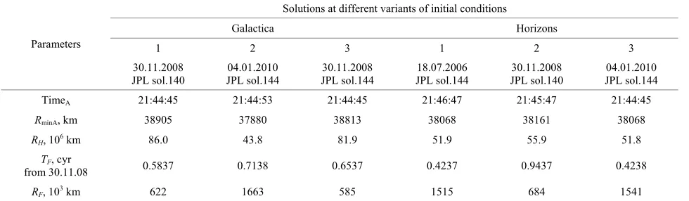
Table 4. Influence of the initial conditions on results of integration of the Equation (1) by program Galactica and of the equations of Apophis motion by system Horizons: TimeA and RminA are time and distance of Apophis approach with the Earth in April 13, 2029, accordingly; RH is distance of passage Apophis with the Earth in April 13, 2036; TF and RF are time and distance of the second approach (point F on Figure 7).

Solutions at different variants of initial conditions

Galactica Horizons 1 2 3 1 2 3

Parameters

30.11.2008

JPL sol.140 JPL sol.144 04.01.2010 JPL sol.144 30.11.2008 JPL sol.144 18.07.2006 JPL sol.140 30.11.2008 JPL sol.144 04.01.2010

TimeA 21:44:45 21:44:53 21:44:45 21:46:47 21:45:47 21:44:45

RminA, km 38905 37880 38813 38068 38161 38068

RH, 106km 86.0 43.8 81.9 51.9 55.9 51.8

TF, cyr

from 30.11.08 0.5837 0.7138 0.6537 0.4237 0.9437 0.4238

RF, 103km 622 1663 585 1515 684 1541

It is seen (Table 4) that the results of the third variant differ from the first one much less than from the second variant. In the second variant the change of positions and velocities of acting bodies since November 30, 2008 for 04.01.2010 is computed under DE406, and in the third variant it does under the program Galactica. The initial conditions for Apophis in two variants are determined according to alike JPL sol.144, i.e. in these solutions the IC differ for acting bodies. As it is seen from Table 4, the moment of approach in solutions 2 and 3 differs on 8 seconds, and the approach distance differs on 933 km. Other results of the third solution also differ in the greater degree with second ones, in comparison of the third solution with first one. It testifies that the diffe- rences IC for Apophis are less essential in comparison with differences of results of calculations under two pro- grams: Galactica and DE406 (or Horizons).

So, the above-mentioned difference of the initial con- ditions (variants 1 and 3 tab. 4) do not change the time of approach of April 13, 2029, and the distance of approach in these solutions differ on 102 km. Other characteristics:

RH, TF and RF also change a little. Therefore it is possible to make a conclusion, that the further refinement of Apo- phis IC will not essentially change its trajectory.

The same researches on influence of the initial condi- tions we have carried out with the integrator of NASA. In system Horizons (the JPL Horizons On-Line Ephemeris System, manual look on a site

http://ssd.jpl.nasa.gov/?horizons_doc) there is opportu- nity to calculate asteroid motion on the same standard dynamic model (SDM), on which the calculations in pa- per [4] are executed. Except considered two IC we used one more IC for Apophis at date of July 12, 2006, which is close to date of September 01, 2006 in paper [4]. The characteristics and basic results of all solutions are given in Table 4. In these solutions the similar results are re- ceived. For example, for 3-rd variant of Horizons the

graphs R in a Figure 7 up to T = 0.45 centuries practi- cally has coincided with 2-nd variant of Galactica. The time of approach in April 13, 2029 changes within the bounds of 2 minutes, and the distance is close to 38,000 km. The distance of approach in April 13, 2036 changes from 52 up to 56 million km. The characteristics of se- cond approach for 100 years changes in the same bounds, as for the solutions on the program Galactica. The above- mentioned other relations about IC influence have also repeated for the NASA integrator.

So, the calculations at the different initial conditions have shown that Apophis in 2029 will be approached with the Earth on distance 38 - 39 thousand km, and in nearest 100 years it once again will approach with the Earth on distance not closer 600 thousand km.

8. Examination of Apophis’ Trajectory in

the Vicinity of Earth

In order to examine the Apophis trajectory in the vicinity of Earth, we integrated Equation (1) over a two-year pe- riod starting from T1 = 0.19 century. Following each 50

integration steps, the coordinate and velocity values of Apophis and Earth were recorded in a file.

The moment TA at which Apophis will most closely

approach the Earth falls into this two-year period. The ellipse E0E1 in Figure 8 shows the projection of the

two-year Earth’s trajectory onto the equatorial plane xOy. Along this trajectory, starting from the point E0, the Earth

will make two turns. The two-year Apophis trajectory in the same coordinates is indicated by points denoted with the letters Ap. Starting from the point Ap0, Apophis will

travel the way Ap0Ap1ApeAp2Ap0Ap1 to most closely ap-

proach the Earth at the point Apeat the time TA. After that,

the asteroid will follow another path, namely, the path

ApeAp3Apf.

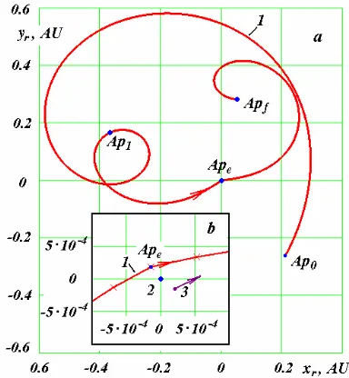
Figure 8. The trajectories of Apophis (Ap) and Earth (E) in the barycentric equatorial coordinate system xOy over a two-year period: Ap0 and E0 are the initial position of Apo- phis and Earth; Apf is the end point of the Apophis trajec- tory; Ape is the point at which Apophis most closely ap- proaches the Earth; the coordinates x and y are given in AU.

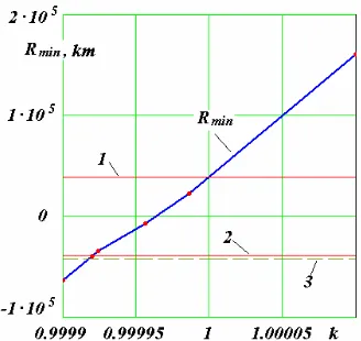
Figure 9. Apophis’ trajectory (1) in the geocentric equato-rial coordinate system xrOyr: a—on the normal scale, b—on magnified scale on the moment of Apophis’ closest appro- aches to the Earth (2); 3—Apophis’ position at the moment of its closest approach to the Earth following the correction of its trajectory with factor k = 0.9992 at the point Ap1; the coordinates xr and yr are given in AU.

the Earth. Here, the relative coordinates are determined as the difference between the Apophis (Ap) and Earth (E) coordinates:

;

r Ap E r Ap

y y y x x x

Along trajectory 1, starting from the point Ap0, Apo-

phis will travel to the Earth-closest point Ape, the trajec- tory ending at the point Apf. The loops in the Apophis trajectory represent a reverse motion of Apophis with respect to Earth. Such loops are made by all planets when observed from the Earth (Smulsky 2007).

At the Earth-closest point Ape the Apophis trajectory shows a break. In Figure 9(b) this break is shown on a larger scale. Here, the Earth is located at the origin, point 2. The Sun (see Figure 8) is located in the vicinity of the barycenter O, i.e., in the upper right quadrant of the Earth-closest point Ape. Hence, the Earth-closest point will be passed by Apophis as the latter will move in be- tween the Earth and the Sun (see Figure 9(b)). As it will be shown below, this circumstance will present certain difficulties for possible use of the asteroid.

9. Possible Use of Asteroid Apophis

So, on April 13, 2029, we will become witnesses of a unique phenomenon, the pass of a body 31 million tons in mass near the Earth at a minimum distance of 6 Earth radii from the center of Earth. Over subsequent 1000 years, Apophis will never approach our planet closer.

Many pioneers of cosmonautics, for instance, K. E. Tsi-olkovsky, Yu. A. Kondratyuk, D. V. Cole, etc. believed that the near-Earth space will be explored using large manned orbital stations. Yet, delivering heavy masses from Earth into orbit presents a difficult engineering and ecological problem. For this reason, the lucky chance to turn the asteroid Apophis into an Earth bound satellite and, then, into a habited station presents obvious interest.

Among the possible applications of a satellite, the fol- lowing two will be discussed here. First, a satellite can be used to create a space lift. It is known that a space lift consists of a cable tied with one of its ends to a point at the Earth equator and, with the other end, to a massive body turning round the Earth in the equatorial plane in a 24-hour period, Pd = 24 × 3600 sec. The radius of the sate- llite geostationary orbit is





2 2

3 _4π

42241 km 6.62

gs d A E

Ee

R P G m m

R

 

  (16)

In order to provide for a sufficient cable tension, the massive body needs to be spaced from the Earth center a distance greater than Rgs. The cable, or several such ca- bles, can be used to convey various goods into space while other goods can be transported back to the Earth out of space.

If the mankind will become able to make Apophis an Earth bound satellite and, then, deflect the Apophis orbit into the equatorial plane, then the new satellite would suit the purpose of creating a space lift.