Nonrecursive digital image restoration

A ~~esis presented for the degree of

Doctor of Philosophy in Electrical Engineering in the University of Canterbury,

Christchurch, New Zealand.

by

M.J. McDONNELL B.Sc. (Hons} ~

ABSTRACT

The problem of digitally restoring blurred images is considered. The subject of image restorati?n is reviewed in detail and a comprehensive notation for image restoration is developed. Degraded images are divided into classes

~and

~ - those which are and are not respectively truncated by their recording frames. It is shown that conventional

restoration techniques only work well for images of

class~­

Restoration techniques for dealing with class ~images are presented, as well as improved techniques for dealing with class

zl

images. These new techniques are shown to be both efficient and practical through the use of computer

simulations, and through the restoration of optically degraded images.

-The problem of designing an optimum nonrecursive

digital filter array of a given number of elements is solved in both one and two dimensions. It is demonstrated that this new design method is superior to previous techniques.

A sampling theory appropriate for deconvolution problems is presented. New sampling functions are

introduced, in both one and two dimensions, which overcome the "picket fence" effect associated with the sine sampling function. The concept of a "line-segment-limited" function is defined. It is shown that a pseudo noise level is

introduced by the approximation that the point spread

ACKNOWLEDGEMENTS

I am deeply indebted to my supervisor, Professor R.H.T. Bates, for his enthusiastic guida~ce and encourage-ment, and also for many useful discussions during the

course of this project. I also wish t6 thank Dr T.M. Peters who supervised me for some months while Professor Bates was

on sabbatical leave ..

I am grateful to my colleagues Dr P.T. Gough, Mr D.J.N. Wall and Mr R.M. Lewitt in the Electrical

Engineering Department for many stimulating discussions on aspect~ of this work. I especially wish to thank

Mr W. K .. ; Kennedy for his valuable assistance. The assistance received from a number of

organisations is gratefully acknowledged. In particular I wish to thank Detective Superintendent E.G. Perry and

.

Detective Inspector J.W. Wooders of the Christchurch Police District, Mr G.R. Scott of the Chemistry Division DSIR in Christchurch, and also the Medical Physics Department of the Christchurch Hospital for use of the electrostatic lineprinter.

I wish to thank my wife Elizabeth for her ·patience and encouragement.

The financial support of a postgraduate scholarship from the University Grants Committee is gratefully

..

TABLE•OF CONTENTS _{, .}

-Page

ABSTRACT ii.

ACKNOWLEDGEMENTS iv.

GLOSSARY ix.

PREFACE xvii.

CHAPTER 1: REVIEW OF IMAGE RESTORATION 1

1.1 Introduction 1

1.2 The Problem 2

1.3 Psf Identification 6

1.3.1 Using zeros of H 6

1.3.2 Edge analysis 7

1.3.3 Image segmentation 8

1.3.4 Calibration techniques 10

1.4 Digital Image Restoration 1 1

1.4.1 Recursive techniques 12

1.4.2 Nonrecursive techniques 13

1.4.2.1 Fourier methods 14

1.4.2.2 Direct methods 18

1.4.3 Positive restoration and superresolution 19 1.4.3.1 Positive restoration 19

1.4.3.2 Superresolution 22

1.4.4 Miscellaneous methods 23

1.4.4.1 Matrix methods 23

J.5 Optical Image Restoration

1.6 Comparison of Optical and Digital Methods

CHAPTER 2: COMPREHENSIVE NOTATION AND DISCUSSION OF SOME IMAGE RESTORATION PROBLEMS

Page

29 31

35 2.1 A Comprehensive Notation for Image Restoration 35 2.2 Circular Property of Convolution Using the FFT 40 2.3 Problems Associated with Class~ Images 41 2.4 Some Problems Associated with Optical

Image Restoration

CHAPTER 3: RESTORATION OF CLASS~ IMAGES 3.1 The Problem of the Zeros of H 3.2 Overcoming the Zeros of·H by

Analytical Inverse Filtering

3.2.1 A decontamination procedure 3.2.2 Analytical inverse filtering 3.2.3 Results of computer simulations 3.3 Simplified Restoration of Images

Degraded by Uniform Linear Motion 3.3.1 Results

43 52. 52 53 56 57 60 61 64

CHAPTER 4: RESTORATION OF RECTANGULAR CLASS ~ IP'illGES 6 9 4.1 Introduction

4.1.1 Modulation transfer function 4.2 One-dimensional Theory

4.2.1 Full edge exte~sion

4.2.2 Overlapped edge extension

4.3 Two-dimensional Edge Extension Theory 4.4 Discussion of Theory

4.5 Practical Examples

4.5.1 Image restoration system 4.5.2 Psf identification

4.5.3 Examples of restorations 4.5.4 Discussion

CHAPTER 5: GENERALISATION OF EDGE EXTENSION METHOD TO INCLUDE ZEROS OF H

5.1 Introduction

5. 2 · Rectangular Class

C§

Images Degraded by Uniform Linear Blur

5.3 Class C§Images in Circular Frames 5.4 Constrained Edge Extension Method

for 1-D Class

C§.

images

5.4.1 Results and discussion

CHAPTER 6: NONRECURSIVE IMAGE RESTORATION USING A FINITE FILTER ARRAY 6.1 Introduction

6.2 Review of Criteria for Deriving a Finite Filter Array

6.3 An Improved Criterion 6.4 Noise Effects

6.5 Sampling Considerations

6.6 One-dimensional Results and Discussion 6.7 Two-dimensional Results and Discussion

CHAPTER 7: A SAMPLING FUNCTION APPROPRIATE FOR DECONVOLUTION

7.1 INTRODUCTION

7.2 Preliminary Discussion 7~3 One-dimensional Theory 7.4 Two-dimensional Theory 7.5 Conclusions

CHAPTER 8: CONCLUSIONS AND SUGGESTIONS FOR FURTHER RESEARCH

8.1 Concluding Remarks

8.2 Suggestions for Further Research i·.

REFERENCES

Page

157

164-168

170 1·70 170

3LOSSARY

Listed below are those symbols used in this thesis which are not always defined in the immediate context in which they are used.

FFT FIR FT MSE MTF psf PSWF SI

sv

1-D 2-D A A' J4?Cx,y) b(x,y) b(r;S) bm (r) b m,n "' b(x,y) B(u,v) B(p;¢)

fast Fourier transform finite impulse response Fourier transform

mean-square error

modulation transfer function point spread function

prolate spheroidal wave function spatially invariant

spatially varying

one dimension or one-dimensional two dimensions or two-dimensional extent of

r

in x-direction

extent of

r

in y-direction available degraded image ideal degraded image

b(x,y) in polar coordinates

the mth term in the angular Four~er series expansion of b(r;8)

the nth coefficient in the Fourier-Bessel series expansion of b (r)

m an estimate of b(x,y) · FT of b (X , y)

B

(u, v)

c (x,y)

c (x)

r

comb(x)

C(u,v)

c

_n

~P}

e

e (x,y)

e' (x)

A

e(x) "i

e (x)

E (u,v)

E

m

A

E

m

~UB (u)

E

uBm f(x,y)

f.

J

FT of b (r) m

,..

FT of b(x,y)

contamination in f(x,y)

the part of c(x,y) in 1-D which is not removable

the part of c(x,y) in 1~D which is removable 00

=

L: o(x-n) n=-oo

FT of c(x,y)

FT of cr(x)

Noise amplification factor

maximum acceptable noise amplification factoi preliminary degradation of p

exponential constant

ideal overlapped degraded image defined by. (5.4)

an approximation to e(x,y) in 1-D initial estimate of e(x)

FT of e (x,y)

mth sample of E(u) mth sample of E(u)

upper bound on !E(u)

I

mth sample of EuB(u}

final degraded image

f "'

,.;

f(x)

fB(x,y)

F (u 1 v)

F m1n

FB (u1 v)

G1G

I

h(x1y)

h(x 1yla, 13)

h (r)

h. k J I

hB(x1y) hc(x1y) hs(x,y)

h

,....,

h(x,y) H(u,v)

H ( p)

sample of f(x,y)

column vector (f.)

J

estimate of f(x1y) in 1-D

decontaminated blurred image in 1-D

inverse FT of FB(u,v)

FT of f (x, y)

sample of F(u,v)

sample of F(u,v) 1n 1-D

result of bandlimiting F(u1v)

Fourier space

real variables

-the general cla:ss of degraded images which are truncated by their recording frames SI psf

SV psf

sample of h(x,y) in 1-D

radially symmetric psf sample of h(x,y)

inverse FT of HB(u,v)

the line-segment-limited psf

the sampled psf

column vector (hj}

inverse psf (inverse FT of H(u,v}) FT of h(x1y)

H(u,v) inverse filter

result ~f bandlimiting H(u,v) mth sample of H(u)

i

=

r-1

I set of integers

set of positive integers

image space

j,k,l,m,n,j ,k integer variables

· m m

J (.)

m

L

n (x, y)

n.

J

t

n.

I J

p(x,y) p(r;8)

p. _{J ,} k

"

p(x,y)

pk P(u,v)

nth positive zero of J (·)

m

mth order Bessel function of the first kind

integer constants

real constant defined in (3.6) extent of T in x-direction extent of T in y-direction

frame function defined by (2.8) noise in f(x~y)

jth sample of n(x,y) in 1-D

jth sample of noise after filtering

Nyquist frequency corresponding to f(x,y)

number of positive zeros of H(p) under consideration

original image

p(x,y) in polar coordinates sample of p(x,y)

estimate of p(x,y)

P(p;<j)) PB(u,v) p uBm P(u,v) r rect(x) s(x,y) s 2(x,y) sqn(x) sinc(x) step(x) t(x,y) t

T ( •)

a

u,v

FT :of p (r; 8) '

result of bandlimiting P(u,v) '-·'

mth sample of P(u)

mth term in truncated angular Fourier series expansion of_P(p;¢)

an upper bound on IP I m FT of p(x,y)

polar radial coordinate in

~

=

1,

=

0,

set of positive real numbers

resultant psf

1-D sampling function for line-segment-l~mited functions

2-D sampling function for line-segment-limited functions

= -1, x<O

=

0, X

=

0

=

1 1 X > 0

=

sin(nx)/nx

=

0, X < 0

=

1 1 X ~ 0.

special class·of degraded images which are not truncated by their recording frames truncated ideal image

as superscript denotes matrix transpose non-linear operator

u ·u' c'. c u m I w,w m w' (x)

w n ~I x,y z(x,y) Z(u,v)

a.,B

y

r

f/'¥ l>(x,y) -/).

e

frequency cutoffs

roth sample of u

real constants

window function defined by (5.3~) sample of

Ji

filter array

ideal filter array

Cartesian coordinates in

~

roth sampling position on x-axis

real constants

amplitude distribution of coherent light incident on front focal plane

FT of z(x,y) dummy variables

arbitrary point in

~

film gamma

frame containing f(x,y)

= {X: X €. f, X

¢.

'¥} Dirac delta function sampling distance

sampling distance adequate to display detail of interest in p(x,y)

roth right half plane complex zero of H{u)

complex component of z;;m

0 A

n;r

1T II p T T w

*

I · I

a;ax

E:

co

v

finite domain of

~

frame containing b(x,y}

= {y: yE.S1, r¢r}

· real constant real part of I:;

m defined by (3.6) real constant

indicates product of terms

polar radial coordinate in

~

· noise level due to approximation h

=

he

original noise level on f

maximum acceptable noise level indicates summation

psf frame

inverse psf frame

6T

polar angular coordinate in ~·

=

lc(x,y) 1/IP(x,y} I

frame containing p(x,y} for a class~ image arbitrary point in

~

frame containing p(x,y}

superscript denotes complex:conjugate modulus

differential with respect to x belongs to (a ~et}

.denotes convolution infinity

is equivalent to

PREFACE

During the last two decades, dramatic advances in technology have made practical the widespread use of

sophisticated signal processing techniques. This is mainly due to increases in the availability, size and speed of digital computers, and to the development of efficient algorithms such as the fast Fourier transform algorithm

(FFT). For example, using the FFT i t is possible to do in minutes computations that would otherwise have taken years.

This progress in signal processing techniques has made i t feasible to process images in a computer, and the

space program has given impetus to research in this area. Image processing has applications not only in aerial

photography but also in other areas such as electron

microscopy, medical imaging and astronomy. A problem which often occurs in each of the above areas is that an image may be unavoidably blurred in such a way that i t is difficult to extract the required information from i t visually. In

generaL this information is not lost, but is masked by the blurring. It is therefore of interest to study image

restoration which is concerned with removing the blurring. Image restoration may be performed by a combination of holography and standard photographic and optical

that. i t can be stor~d as discrete "pixels" (picture elements) in. computer me~no~y '- the restoration is then

t:,-,

carried out in a digital computer. The interest in this thesis is in digital techniques which, in my experience, are superior to optical methods because of their greater versatility and accuracy.

This thesis is concerned with the development of efficient techniques for the digital restoration of blurred images. It is shown that conventional image restoration techniques are unsatisfactory, and· new restoration

techniques are developed which overcome the deficiencies of conventional methods. New material is included in

chapters 2-7.

In chapter 1, the subject of image processing is reviewed in detail. The problem is defined, and methods of deducing the point spread function characterising the blurring are reviewed. Digital and optical image

restoration techniques are reviewed separately and finally compared.

In chapter 2, a comprehensive notation for use in image restoration is introduced. In addition, some of the problems associated with conventional restoration techniques are discussed. Degraded images are divided into the classes

~and

.d. -

those that are and are not respectively

property of convolution, which is exhil::?ited when the FFT is used, is also discussed.

· A problem which sometimes occurs in the restoration of class ~ images is that zeros of the modulation transfer

function (MTF) of the blurring may lie on sampling points. In chapter 3, this problem is discussed in general and i t is shown in particular how i t may be overcome in the case of uniform linear blur.

T\vo techniques for the restoration of rectangular class ~images are presented in chapter 4. The better of these two methods is illustrated with a number of

restorations of optically degraded images. This technique is shown to be practical and very efficient.

In chapter 5, i t is shown how the simple but effective methods of chapter 4 can be modified to take advantage of knowledge of the zeros of the MTF. The

·resulting restoration method is shown ·to be less efficient but more accurate than the best method of chapter 4.

A simple technique is presented for the restoration of class ~images degraded by uniform linear blur. The possibility of restoring class ~images recorded in

circular rather than rectangular fram~ is also considered. It is possible to restore degraded images· by direct convolution with a nonrecursive digital filter array of finite length. This is considered in detail in chapter 6 and an improved technique is described for deriving an optimum finite filter array of a given length.

deconvolution is presented. New sampling func~ions are introduced,-in both one and two di~ensions, which overcome

r.' •

the "picket fence" effect associated with the sine sampling function. The concept of a "line-segrnent'limited" function is defined. It is:_ shown that a pseudo noise level is

introduced by the approximation that the point spread

function is line-segment-limited. It is this pseudo noise level, and not aliasing errors, that restricts the choice of a sampling rate less than the Nyquist rate. New criteria are presented which allow the choice of a sampling rate considerably less than the Nyquist rate.

Chapter 8 consists of concluding remarks and some suggestions for further research and development relat~d to the results presented in this thesis.

Papers co:r:npleted to date on topics relevant to the material presented in this thesis are as follows:

Stedman, G.E., McDonnell, M.J. 1973 "Optimisation of coherence properties of thermal sources by spatial filtering, 11 _{J. Opt. Soc.}

Am. 63, 1222-1224. Bates, R.H.T., Kennedy, W.K., McDonnell, M.J. 1974

"Efficient digital restoration of images blurred by linear motion," Letters in Applied and Engineering

Sciences~' 133-143.

McDonnell, M.J., Bates, R.H.T. 1975 "Preprocessing of degraded images to augment existing restoration methods," Computer Graphics and Image Processing

McDonnell, M.J., Bates, R.H.T. 1975 "Restoring parts of scenes from blurred photographs," Optics

Communications ~, 347-349.

McDonnell, M.J. 1975 "Nonrecursive image restoration using a finite filter array," Optik 43, 159-174. Bates, R.H.T., Napier, P.J., McKinnon, A.E., McDonnell, M.J.

1975 "Self-consistent deconvolution: I: Theory," to be published in Optik.

McKinnon, A.E., McDonnell, M.J., Napier, P.J., Bates, R.H.T. 1975 "Self-consistent deconvolution: II:

Applications," to be published in Optik.

McDonnell, M.J. 1975 "A sampling function appropriate for ·deconvolution," to be published in IEEE Trans. on

.. Information Theory.

McDonnell, M.J., Kennedy, W.K., Bates, R.H.T. 1975

"Identifying and overcoming practical problems of digital image restoration," submitted to the

New Zealand Journal of Science.

McDonnell, M.J., Bates, R.H.T. 1975 "Digital restoration of an image of Betelgeuse,"

Ap. J.

submitted to

"CHAPTER ONE

REVIEW OF IMAGE "RESTORATION

1.1 INTRODUCTION

The subject of image processing is interdisciplinary. It has been defined by Huang, Schreiber and Tretiak (1971) as dealing with the manipulation of data which are

inherently tvm-dimensional (2-D) in nature. It includes image restoration, image enhancement, pictorial pattern recognition and image coding, and also finds application in such diverse areas as medical imaging (Hallet al 1971, Mersereau and Oppenheim 1974), space exploration and aerial reconnaissance (Sawchuk 1973), electron microscopy (Saxton 1974), astronomy (Bates and Gough 1975), geophysics (Backus _. .

and Gilbert 1970) and police work.

The interest here is in image restoration, which is closely allied to image enhancement. Some authors (Stroke 1972, Frieden 1973) consider these two subjects to be

identical, while others (Huang et al 1971) take image· restoration to be part of image enhancement. In general, however, as in this thesis, the two subjects are treated as distinct (Andrews 1974, Billingsley 1973, Rosenfeld 1972).

visually apparent before processing (this improvement may include such aspects as noise reduction, compensation for no nlineari ties of the recording medium, contrast adjustment, edge sharpening, etc.). Image restoration is concerned with the reconstruction of an ideal or original image by

inversion of some degradation processes. It usually

involves the uncovering of information which has been masked by the degradation. Once a degraded image has been restored, i t may be desirable to use enhancement techniques to improve its display.

Image restoration techniques are classified as a posteriori or a priori. In the former, the restoration is carried out after the degradation has occurred. In the latter'· the imaging system is designed so as to minimise the effect of an anticipated degradation, or to simplify

subsequent application of a posteriori techniques. A priori methods have found their widest applications in attempts to overcome the effect of atmospheric turbulence on

astronomical imaging (Labeyrie 1970, Bates and Gough 1975), and also in compensating for camera motion (NASA/ERC

Seminar 1968). Shutter modulation techniques (Bryngdahl and .Lohmann 1 968) have also been proposed for modifying the

degradation. A priori methods have usually been designed for particular applications. In this thesis the interest is in the more general a posteriori methods.

1.2 THE PROBLEM

are considered to ~e 2-D and, for- simplicity, ~ono~hromatic. Such an imag~ is represented ~s a real function of two

coordinates (x,y) representing the intensity of the images at a point in image space

~

The ideal image that would be obtained with a perfect recording system is denoted as

'

.•-p = p(x,y). Since any practical recording system is imperfect, the available image is necessarily degraded. It is denoted

by~~x,y).

The purpose of image restoration is to obtain

from~n

estimate of p. This estimate vlhich is denoted by

p

=

p

(x, y), minimises in some sense- e.g., the mean-square error (MSE) criterion (Sandhi 1972) the difference between itself and p.

The degrading system could conceivably be very

complicated. However, in certain cases which have practical application i t has been modelled (Huang et al 1971) by the block diagram shown in Fig. 1.1.

The ideal image p is acted on by a linear system with an impulse response, or point spread function (psf), which is spatially varying (SV). At a general spatial point (a,8) this psf is given by h

=

h(x,y,a,8) so that

00

b

=

b(x,y)

=

ff

h(x,y,a,8)p(a,8)dad8. ( 1 . 1 )

_oo

The available degraded

image~s

in general a nonlinear function T (•) of the sum of band the noise n

=

n(x,y),

a

which is usually assumed to be additive (this assumption is discussed in 1.4.4). This gives

=

T (b(x,y) + n(x,y)).

T is a characteri$tic of the detector used to record the a.

intensity of_ the degraded .,image. In practice, an estimate of T is usually available. It is assumed here, as is most

a.

often the case, that the detector is photographic film, so that (1.2) becomes

yf=

(b

+

n) ·

..,f

( 1 • 3)

.where yf is called the gamma of the film (Goodman 1968). It is possible to estimate Yf from the characteristics of the film arid the developer used on the film, and from the

duration of the development time (Goodman 1968).

Harris (1968) has shown that errors in ~fin (1.3} have bnly a slight effect on the quality of restoration~

Therefore most authors (e.g., Sandhi 1972, Frieden 1974) assume that the g~mma can be corrected easily, so that i t makes practical sense to define a final recorded image,

f = f· (X 1 y) 1 by

f

=

b + n. ( 1 • 4)

It is the restoration of p from f. which is the main concern here.

Usually h i s taken to be spatially invariant (SI):

h = h(x,y,a,S)

=

h(x-a.,y-S). ( 1 • 5)

This is often true in practice. When h is SV i t is often possible to define some geometrical or other transformation

In some cases (Huang et al 1971) h varies only slowly with position, so that the image may be segmented (Granger 1968) and considered to be SI over each segment. Some restoration techniques discussed later allow h to be SV. However,

unless stated otherwise, h is assumed in this thesis to be SI. This makes i t possible to express (1.4) as

f

=

.p ®h + n ( 1 • 6)

where ® denotes convolution.

This is now in the form of a general 2-D deconvolution problem. However, because image intensities are being

considered, i t is also true thaf

f,-b,p,h E R+ (1. 7)

where R+ is the field of non-negative, real numbers. This additional condition is used in_"positive" restoration methods which are discussed.in 1.4.3.

It is worthwhile noting here that, by including (1.7), · attention is restricted to incoherent imaging systems (as is

assumed in most of this thesis). However, restoration metbods which do not invoke (1.7) are also applicable to

coherent imaging systems (e.g., phase contrast or amplitude contrast electron microscopy (Erickson 1973)).

The Fourier transform (FT) of a quantity is

identified by the upper case form of the lower case English letter which denotes the quantity, e.g.

00

F

=

F(u,v)

=

If

f(x,y)e2Tii(xu+yv)dxdy,

( 1.

8)

where u and v are the Cartesian coordinates in Fourier space

~and

i

=

1=1.

Coordinates

~in~ay

be interpreted as

spatial frequencies. A component at (u,v) in~orresponds to a sinusoidal variation in~ with frequency components

u

and v in the x and y directions. respectively.

1.3 PSF IDENTIFICATION

In order to solve (1.6) for p i t is necessary to know h. Methods for determining h have been reviewed by Huang et al (1971). Sometimes h i s known from a combination of mathematical analysis together with calibration measurements

of the imaging system (NASA/ERC Seminar 1968, Erickson and Klug 1971) or from knowledge of camera motion during the exposure (NASA/ERC Seminar 1968). The general form of h may, on occasions, be known initially but quantitative details may have to be deduced. In other cases, h may be completely unknown.

1.3.1 Using Zeros of H

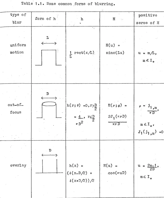
Table 1.1 lists the forms assumed by h for a number of common degradations, following Roetling et al (1968). The table also lists the optical transfer function,

H

=

H(u,v), and the positive points in~t which His

.

rect (x)

=

1 ,

I

X

I

~

!

I

X

I

>

-!

( 1 . 9)

- 0 ,

and I+ is the set of positive integers.

If h i s of a simple (cf. Table 1.1) but unknown form, i t is possible to determine the particular simple form of h from the zeros of IF(u,v)

I

(Gennery 1973). Taking theFT of (1.6), neglecting noise, and using the convolution theorem for Fourier transforms gives

F

=

PH. (1.10)

It follows that the set of zeros of F is the union of the set of zeros of P and the set of zeros of H. If h has a simple form, like any of those in Table 1.1, the zeros of H form a simplepattern (e.g. they lie along equispaced

parallel straight lines for uniform motion blur, or on rings for out-of-focus blur). In general the zeros of P do not form a simple pattern. Therefore, the pattern of the zeros of H is clearly visible among the zeros of F, if !FI is

displayed, so that the form of h may be deduced. For simple blurs, the extent of h may be calculated from the spacing of the zeros (Gennery 1973).

1.3.2 Edge Analysis

edge be modelled as a unit step function step(x) defined by

step(x)

=

0, x < 0,

(1.11)

= 1, X ~ 0,

and consider this edge as the original image. Neglecting noise, f is given by

Now

f(x,y)

=

step(x) 0 h(x,y)

d f {x, 0)

ax

co

=

JJ

step(x-a)h(a,S)dadS.

.. -co

co

=

f

h(x,S)dS

-co

(1.12)

(1.13)

(1.14)

which is the projection of h parallel to the y-axis (Smith et al 197 3). Edges in different directions give different projections of h. An estimate of h may be· reconstructed from a finite number of these projections (Smith et al 1973). If h is circularly symmetric i t may be recovered from a single projection. If h is one-dimensional (1-D) then

(1.13) reduces to

df(x,O)

ax

=

h (x) ,

so that h may be found directly.

1.3.3 Image Segmentation

(1.15)

(1971). It is based on work done by Prof. T.G. Stockham on the restoration of old Caruso recordings. The results of this investigation were later presented in detail

(Stockham et al 1975).

The final degraded image is divided into M segments of equal size, and the intensity distribution in the jth segment is denoted by fj

=

fj(x,y), where j

=

1, ... ,M. The corresponding intensity distribution of the original image in the jth segment is denoted by pj

=

pj(x,y). The effect of convolving pj with h is not confined to the jth segment because the degraded image is spread into adjacent segments. This effect may be reduced by multiplying each segment by a window which falls off to zero at the edge of each segment (Stockham et al 1975). It is then

approximately true that fj ₌ pj _{® h}

I j = 1 1 • • • I M. (1.16)

so that (1.10) gives

Fj ₌ pj _H

_,

_{j = 1 I • • • I M. (1.17)}

Taking the product of (1.17) over j and solving for

IHI

yields

1 1

[.~

Fj]

M

~M

·r

IHI

=

rr

pJ (1.18)

]=1 j=1

I [.

~

pj

1

An a J2riori guess is made at the form of

MJ

I

_so ]=1

that (1.18) gives an estimate of

I

H ' · For simple blurs (as

A refinement of this technique is suggested in chapter B.

1.3.4 Calibration Techniques

One method of determining h which comes under the heading of calibration techniques is proposed by Ekstrom

(1973a). He considers the case when the degraded image f of a known original image p is available. Neglecting noise and using a discrete model of (1.6} he. obtains

(1.19)

where (in matrix notation)

f

=

(fj),

h

=

(hk) and~= (pj,k) for j = 1, ... ,N1 and k = 1, ... ,N2 and where N1 >N2 •

In matrix notation, the convolution in (1.6) corresponds to multiplication of _h by a matrix

R.

of dimension N 1 x N2 •

(A 1-D explanation is given here for simplicity). The method of least squares is then used to obtain an estimate of

h

given by

(1.20)

where the superscript t denotes the matrix transpose. Methods such as this are often used when calibration is

possible. The edge detection methods described in 1.3.2 are the most commonly used when h cannot be determined through calibration. The advantage of the method described in 1.3.3

1.4 DIGITAL IMAGE RESTORATION

Image restoration methods for obtaining p from£, as given by (1.6), are in general either optical or digital. Optical image restoration is performed by a combination of holography and standard photographic and optical techniques. Alternatively, the image can be digitised byscanningit with a computer-controlled microdensitometer, so that i t can be stored as discrete "pixels" (picture elements) in computer memory - the restoration is· then carried out in a digital computer. Digital and optical techniques are reviewed

separately in 1.4 and 1.5 respectively, and are compared in 1 . 6.

Digital image restoration has recently been reviewed by Huang et al (1971), Sondhi (1972), Andrews (1974) and Hunt (1975). It has also featured in a number of special issues of journals (e .·g. Proc. IEEE July 1972, Computer May 1974, and Optical Eng. May-June 1974). Two introductory books have been published on the subject (Rosenfeld 1969, and Andrews 1970).

, Various digital image processing laboratories are in operation and have periodically issued reports describing their facilities and the tasks they carry out (Patterson et al 1974, Hunt et al 1974, Billingsley 1973).

Digital restoration techniques are broadly divisible into four categories: recurs~ve, nonrecursive, positive and superresolution, and miscellaneous. These are dealt with in turn.

due to Andrews (19T4), of restoration techniques into two categories: continuous/continuous methods and

discrete/discrete methods. In the continuous/continuous methods, both f and p are considered to be continuous.

It is then assumed that f is bandlimited, so that the

continuous f may be obtained from t'tle samples of f taken at the Nyquist rate (Goodman 1968). It is said that f is band-limited to a frequency Nf if

IF(u,v) I

=

0 (1. 21)

in 2-D, or

IF (u) I

=

0 _for

I

_{u I} > Nf' (1.22) in 1-D (i.e. for f

=

f(x)). The Nyquist sampling rate in a given direction is equal to the reciprocal of the actual (or effective) extent of F in that direction. In the

discrete/discrete methods i t is assumed that both f and p are sampled and discrete.

1.4.1 Recursive Techniques

A recursive digital filter is one which gives a sequence of output samples as a weighted sum of input samples and previously calculated output samples. Such a

"'

filter may be used to give samples of p from samples of f and previously calculated samples of

p.

In 1-D, if pk and

"' "'

fk {where k€I+) are samples of p

=

p(x) and f

=

f(x) respectively, then in general the pk are given by

= ₊

M2

. r

M d. fk . ,

J =- 2 J -J

where M1 , M2 , the c₁ and the dj are constants. Such filters

are widely used in 1-D signar processing (IEEE Selected Reprints on Digital Signal Processing 1972). A number of approaches have been taken to the problem of extending these filters to 2-D (e.~. Shanks 1970). Some attempts have been made to apply these· 2-D recursive filters to image

restoration (Zimmermann and Gupta 1973, Hall 1972). However, their usefulness has been limited for a number of reasons. Firstly; because of the lack of a 2-D factorisation theorem

(Huang et al 1971), many results for 1-D recursive filters do not hold in 2-D. This makes i t difficult to approximate a desired frequency response with a stable 2-D filter.

Secondly, to be effectively implemented, a 2-D recursive filter needs to be approximated by a finite sum of separable filters (Huang et_ al 1971). A third problem is the choice of boundary values needed to start the recursion. Because the number of sample points in an image is often not large (e.g. 128x128 pixels), the effect of errors in the chosen boundary values may spread throughout the whole image. For these reasons, recursive filters are not much used in image restoration at present.

1.4.2 Nonrecursive Techniques

The use of nonrecursive filters for image restoration is widespread. The outputs of such filters depend only on the input samples. Unlike with nonrecursive filters, there is no feedback of previously calculated outputs as in (1.23). Corresponding to (1.23) the general expression for the

= .(1.24)

where M2 and the d. are constants. The main advantages of

J

these filters are that there is no stability problem, they are easily implemep.ted, noise analysis is relatively simple, and the extent of the resultant psf (i.e. the result of

convolving the psf with the filter) in the restored image can be conveniently chosen. Nonrecursive filters are applied either by convolution in image

space~r

by multiplication in Fourier

space~

1.4.2.1 Fourier Methods

Nonrecursive filtering is carried out in~y means of the Fourier or the Hadamard transforms. Such

transformations have been made practical by the development of efficient alg·orithms for carrying them out on the digital computer. The Fast Fourier Transform algorithm or FFT was put forward by Cooley and Tukey in 1965. Later a fast Hadamard transform also became available (Andrews 1970, Robinson 1972). Only the FFT is considered here because similar results hold for both transforms, and the FFT is the one more widely in use. Other fast transforms such as the Fermat number transform (Agarwal and Burrus 1974) also exist.

Unlike theFT in (1.8) which acts on a continuous function f, the FFT acts on a rectangular array

where

N N

F

m,n

=

1 't' ·,· . ' 27fi(k.m+ln)/N2

L. ~ ' f e

N2 k=1 1=1 k, 1 ·:· • ( 1 • 25) Various Fourier transform filtering techniques which have become known as "inverse filtering" are now discussed. In line with most work on the subject (Huang et al 1971, Andrews 1974) the filtering equations are presented in continuous form, although their digital implementation by means of the FFT is necessarily discrete.

Taking theFT of (1.6) gives

F

=

PH+N. ( 1. 26)

A

In the procedure known as inverse filtering, p is taken to be the inverse FT of F H, where H = H (u,v) is called the "inverse filter" ~or the following reason. When n = 0 i t follows from (1.26) that

p

= p if

H = 1/H, (1.27)

which is known as the direct inverse filter.

Two shortcomings of the direct inverse filter {1.27) are as follows. Firstly, H may have zeros at spatial

frequencies within the range of interest (e.g. uniform motion blur and out-of-focus blur) , in which case 1/H does

not exist. Secondly, division by H tends to unduly amplify any noise that is present at or near zeros of H. This noise amplification tends to increase with frequency because IHI generally decreases with increasing frequency. These

Andrews 1974) and Hunt (1975). A number of aut~ors (Harris 1966, McGlamery 1967, Muelier and F~ynolds 1967) describe restoration techniques using filters which are minor

modifications of (1.27). For example, Nathan (1971) uses (1.27) with the proyiso that His not allowed to exceed a set constant.

When n

f

0, which is always true in practice, perhaps the most suitable form for H is the Wiener filter (Helstrom 1967, Slepian 1967aj Horner 1969)

H

=

H

*

where the asterisk denotes the complex conjugate and

(1.28)

~

=

~(u,v) is an a priori estimate of the ratio of INI to

!Pl.

The Wiener filter is optimum in the sense that i t

.

"

results 1n a p for which

CX)

. J J

I

p

(x, y) - p (x, y) 12 dxdy (1.29)

- CX)

is minimised (Sondhi 1972). A number of modifications to the Wiener filter have been proposed (Hunt 1975, Cole 1973). For example, Cole (1973) suggests a geometric mean filter which can be classed between the inverse filter and the Wiener filter:

H

=

I

*

1-S I

(.!_)s ( H )

H IHI2 + 4>2

( 1 • 30)

where 0 ~ s' ~ 1. Gennery {1973) simplifies (1.28) by

of the noise which he then estimates.

Constrained least squares methods are discussed in 1.4.4.1 for the SV case. The corresponding filter for the SI case is (Hunt 1975)

H

=

H

*

(1.31)

where A is a parameter determined by iteration and

~u,v)~{u,v)

corresponds t o £ in (1.50) (refer to 1.4.4.1).

The MSE criterion in (1.28) for the optimum

p

is not necessarily the best. Optimality criteria are discussed by Sondhi (1972) and Hunt (1975). The restoration procedure yielding the result

p

which appears the best, depen~on

£,

the detail of interest in p, and also on the interpretative powers of the human observer. Thus, human criteria for

judging the best restoration are essentially subjective. However, to be practically implemented, criteria need to be objective. The advantages of the MSE criterion are that i t is objective and easily computable. The problem of

presenting an image in the most suitable form for a human observer is largely an enhancement problem, for which

techniques such as histogram equalisation (Andrews 1974) can be used. Even so, i t is desirable that the optimality

H

=

H

*

(1.32)

where IHel

=

IHe(u,v) I is the modulation transfer function of the eye. Nevertheless, the MSE criterion has been widely adopted and is showA to_ produce good restorations by a

number of authors (Gennery 1973, McGlamery 1967, Harris 19 68) .

1.4.2.2 Direct Methods

Nonrecursive filtering can be accomplished directly by convolution with a finite filter array

in~s

in (1.24). One advantage this offers is that i t is faster than

convolution using the FFT, if the array is small enough (Hall 1972). The main disadvantage is that direct methods lack the versatility of Fourier methods for dealing with noise. Implementation of direct nonrecursive filters can be either digital, or optical, using incoherent light to superimpose displaced negatives (Frieden 1974), or electro-optical by scanning with a specially designed aperture and writing the result directly on to film (Smith 1966, Honda et al 1 9 7 4, 1 9 7 5) .

in 1-D by Smith (1966) when designing a continuous filter rather than a filter array. He minimises the radius of gyration of the resultant psf. However, the solution for a filter array is more useful and this is considered in both one and two dimensions by a number of authors (Saleh 1974, Frieden 1974, Stuller 1972, Riemer and McGillem 1973, Nathan 1971, Arguello et al 1972, and Honda et al 1974, 1975). The various techniques they propose for deriving the filter array and dealing with noise are considered in detail in chapter 6. It suffices to say here that nonrecursive filter arrays provide a viable alternative to Fourier filtering methods.

1.4.3 Positive Restoration and Superresolution

Positive restoration methods make use of (1. 7)- in addition to (1.6) so that the solution is generally more difficult than for the methods previously mentioned._ Superresolution aims at recovering the spatial frequency content of an image that has been lost through bandlimiting. Positive restoration is considered ·here with superresolution because positive restoration methods can be used to obtain superresolution. Positive restoration and superresolution are discussed by Andrews (1972, 1974), Gerchberg (1974) and Huang et al (1971).

1.4.3.1 Positive Restoration

Positive restoration methods have only recently

become available. They have been used with some success in 1-D applications, but their use is not yet practical in 2-D.

technique to achieve superresolution in 1-D. He assumes that P

=

P(u) is given up to some cutoff frequency u , and

. c

wishes to extend P to a new cutoff frequency ur >u. c c

As p

=

p(x) is positive he defines a new function g

=

g(x) by

p(x)

=

(g(x)) 2_~0,

so that

P(u) = G(u)

®

G(u}.

He then develops an iterative technique to find an

A A

estimate G

=

G(u) of G which minimises

where

u

c

I

₀ A 2 cc

I

P < u > - . P c u >

I

a:u ,

P(u)

=

G(u) ® G(u).

(1.33)

( 1 • 34)

( 1 • 35)

(1.36)

P

=

P(u) given by (1.36) is bandlimited to u~ as required. Other authors (Philip 1963, 1973, Frieden 1972,

Frieden and Burke 1972, Lahart 1974) use a maximum likelihood or maximum entropy ·restoration which finds the most likely original image given a degraded image formed from a

statistical distribution. Alternatively, the image may be assumed to be a 2-D probability density function, so that Bayes theorem can be used for the restoration (Richardson 1972}.

intensity increments or":Jrn.ins" at samples of

p.

"

A corresponding estimate f

=

f(x) of the degraded image is cumulatively built up and at any stage is given by

(1.37)

A decision rule is required for the placement of grains. ·A grain of fixed intensity d is placed at a sample x of

o n

"

p if xn permits the inequality

f

(x ) + d h (x -x ) ~ r

f

(x )

m o m n m m ( 1 • 38)

to be obeyed for all samples x , for a minimum value of m

r . This method gave encouraging results in a computer

m

simulation, but is not yet practical for use in 2-D. Another technique which is classified as positive by Andrews (1974) is the modified Van Cittert method used by Jansson (1970) and Jansson et al (1970). Neglecting noise, the 1-D form of (1.6) may be written as a matrix equation

(1.39)

where in matrix notation f

=

(f.) and p

=

(pk) are column

J ,...,

rectors of length N, and H

=

(h. k) is a square matrix.

- Jr .

Attempts to solve (1.39) directly by inversion of~ to yield

-1

= _,... H f (1.40)

lead to unacceptable solutions because of the instability of H to inversion. An iterative technique is therefore

,_.

"k

k+1

The p. are obtained from

J

"k+1

p.

J

=

"k

P·

J + (1.41}

"'1

where K is a relaxation parameter and

,e

=

.f.

This approach

has given good results when applied to physical spectra in 1-D. However, i t would be unwieldy in 2-D because of the size of the matrices that would be involved.

1.4.3.2 Superresolution

Analytic continuation is the principal method of obtaining superresolution. The basis of the approach is that the FT of an image of finite extent is analytic, so that the whole FT can be obtained, in the absence of noise, from any portion of i t . Prolate spheroidal wave functions

(PSWF's) are ideally suited to analytic continuation (Slepian and Pollak 1961). They are used for superresolution by

.a

number of authors (Frieden 1967, Barnes 1966, Rino 1969, Huang et al 1971). An earlier technique not using PSWF's was discussed by Harris (1964). The main limitation of

these methods is that they are very unstable in the presence of noise and only a very small extension of the FT seems to be practical (Rushforth and Harris 1968). Once again

experimental results have been restricted to 1-D: It seems clear that the iterative approach of

It is assumed that the extent of p(x} is less than or equal to A.

P. (u)

J

The (j+1)th estimate Pj+

1 (u) of P(u) is obtained from as follows. Take the inverse FT of P. (u) to obtain

J

p . (x) •

J Obtain pj+1 (x) from

Pj +1 (x)

=

Pj(x) rect(x/A).

Then P.+

1 (u) is given by

J .

P j+1 (u)

=

=

_{E'T of Pj+ 1 (x),}

( 1. 42)

I

(1.43) The resultant error after each iteration Rj+

1(u) is given by

P j+1 (u) = P (u) + Rj+ 1 (u) . (1.44)

Gerchberg shows, using Parseval's theorem, that the 'energy' of the error spectrum is monotonically decreasing as j

increases. The technique is surprisingly stable to noise and the results are limited more by the accuracy of the

estimate of the extent of the image, than by the noise level present. De Santis et al (1975) have reformulated

Gerchberg's algorithm using PSWF's.

1.4.4 Miscellaneous Methods

1.4.4.1 Matrix Methods

In 1-D (1.4) may be written using (1.1} as

00

f(x)

=

f

h(x,a)p(a)da + n(x), (1.45)

which is in the form of a Fredholm integral equation of the first kind. The discrete/discret~ version of (1.45) is

f

=

H p + n

,..., ~ ,...., (1.46)

where (in matrix notation) f

=

(fj)'

£

=

(pk)'

n

=

(nk) ' H

=

(h. k) for j

=

1, .. , Nand k

=

1, .. , M. A number of

-

] ,

numerical analysis techniques have been proposed for solving this equation for

p

=

(p.),

j

=

1, .. , N. As written, (1. 46)

. - J

describes an SV system. When h is SI, the Fourier inverse filtering techniques of 1.4.2.1, using the FFT, become applicable with a consequent increase in processing speed.

In continuous form (1.45) has no stable solution because a high frequency oscillation in p can produce a negligible effect on f (Phillips 1962, Sondhi 1972). If f and p are sampled at rates such that N

=

M, if n

=

0, and if the determinant of His nonzero, then in principle (1.46) _...,.

A

is solvable for p. However, in practice, because of the size of N, inversion of

E

is slow, andE is almost singular

(Hunt 1972, Ekstrom 1973b,c). This makes the solution very unstable in the presence of noise. If (1.1) is expressed in matrix form in 2-D, with the 2-D matrices being rewritten as 1-D ones (MacAdam 1970, Hunt 1973), the problems become even worse (Andrews 1974, Huang et al 1971).

As well as the technique of Jansson et al (1970) characterised by (1.41), pseudoinverse techniques (Adler

where

k

= ₁₌₀ E (I-H) lf

~ """ , . . J (1.47)

or

₌

f + (I-H)""k-1 .~ ~ p I (1.48)

where I is the identity matrix. Such iterations, although slow, are capable of giving, in 1-D, a _{,.._}

p

which is a

considerable improvement on

L·

It is possible to solve (1.46) by placing constraints on it. Phillips (1962) proposes that the £be found which A is the smoothest solution in the sense that

co

(1.49)

is minimised. Twomey (1963) gives a more generalised solution which does not require H to be square. _~ He puts a constraint on the noise and the smoothness, obtaining

" _{(HtH C)- 1 Htf, (1.50)}

p = +

... ...,. ,..._. ll,...,. ,_, ,_

where

c

= p Cp t _{is minimised, where £is} some square matrix

p _...,

~---that makes Cp a reasonable criterion of smoothness. ~ is chosen by trial and error to give the best solution.

Setting~= 0 in (1.50) results in

=

(1.51)

which is a direct inverse filter generalised for the SV case. Corresponding generalisations of the Wiener and other

two major disadvantages, ncmeiy lack of speed and impracticability in 2~D.

MacAdam (1970) shows how any 2-D convolution can be rew·ri tten as a 1-D ~onvolution. He then develops an

algorithm for doing deconvolution under the constraint that

"

the values of p, f, and h lie within prescribed ranges. He suggests that the constraints should be modified after each attempt at a restoration. The danger here is that the

programmer may end up partly drawing his own picture. The main disadvantage of the method is its slowness, if f has a

large number of samples. 1.4.4.2 Other Methods

A technique which has found some application in 1-D image restoration ·(McKinnon et al 1975, Bates et.al 1975) is based on the following result. A function of finite

extent is characterised uniquely by the zeros of the complex FT (Bates 1969). The complex FT is defined as in (1.8). except that u and v are complex. The basic result is that the set of complex zeros of bin (1.1) is the union of the sets of complex zeros of p and h. Thus, deconvolution may be performed by subtracting the. set of complex zeros of h

"'

.

from that of b, and then obtaining the corresponding p 1n image space.

A number of authors consider the case when h(x,y,a,B) is not deterministic, but a ~andom function of position

Another possibility known as multiframe processing is that

a

number of images of a single object may be

available, each of which has been degraded by a different psf. The various methods proposed for dealing with this case are discussed by Huang et al (1971}. However, the main interest in this thesis is with a single image

degraded by a deterministic psf.

The restoration techniques discussed so far are linear. However, nonlinear techniques for restoring

linearly degraded images are also possible. Frieden {1968) derives a filter to minimise

00

If

jp(x,y) - p(x,y) 1· dx dy, " . K· (1.52}

-co

instead of (1.29), where K is a positive integer.

A thorough treatment of nonlinear filtering techniques is given by Oppenheim et al (1968). Their use is demonstrated to be practicable by Stockham et al (1975). However, non-linear techniques, though potentially more powerful than linear ones, have not yet found wide application because the slight processing advantages they offer are ~utweighed by their increased complexity and decreased speed.

In (1.4) the noise present in f is assumed to be additive. Although this is the simplest and most commonly used model, i t is not necessarily the most accurate one. Some types of noise are better modelled as being

multiplicative (Huang 1966, Hunt 1975). Both Stockham (1972) and Hunt (1975) consider ways of dealing with

the effects of various types of noise in a system. However, at present, image restoration quality seems to be limited more by the image restoration technique used than by the

inaccurate model of additive noise.

In each restoration technique which has been discussed, except for direct nonrecursive filtering and the slow matrix methods in 1.4.4.1, i t is effectively

assumed that all o f f given by (1.4} is available. However, any real-world image must be of finite size because i t

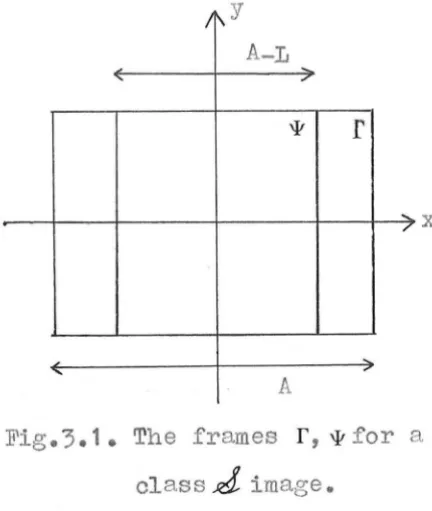
exists within a finite recording .frame. As is explained in detail in chapter 2,· i t makes sense to consider the special class

.d.

of degraded images which, fit completely inside their recording frames; and the general class~of degraded images which are truncated by their recording frames. In the case of class~images, the restoration techniques which have been discussed (except for direct nonrecursive filtering and the slow·matrix methods in 1.4.4.1} are unsoundly based and may give unacceptable results.

This serious problem is mentioned but not solved by Huang et al (1971), Ekstrom (1973c}, Hoppe (1970), Lewis et al (1975), and Campbell et al (1974). It is discussed in detail in chapter 2. In almost all published restorations

truncation of f because i t is of class~only has an effect on a band at the edge of

p,

whose width equals the width of the filter array. This is noted by Ekstrom (1973c).

1.5 OPTICAL IMAGE RESTORATION

Vander Lugt (1968), Stroke (1972), Huang et al (1971) and Campbell et al (1974) are among the many who have

reviewed optical image restoration techniques, which are usually effected with a coherent optical system similar to that shown in Fig. 1.2.

The FT property (Goodman 1968) of a lens means that if a film tra~sparency with amplitude transmittivity f(x,y) is placed in the front focal plane (a) of lens (b) , and is illuminated with a collimated uniform beam of coherent monochromatic light, then the amplitude at the back focal plane (c) of lens (b) is

F(21T~l 21Tnl

Af '~) - 1 1

=

F(u,v) (1.53)

where (~1 _,n1 _{) are the spatial coordinates of the back focal}

plane, X is the wavelength of the light, and f₁ is the focal length of each lens. This means that inverse filtering may be performed optically simply by placing a film transparency, whose amplitude transmittivity is equal to the desired

filter H, in the back focal plane (c) of lens (b} (Goodman 1968, Stroke 1972). A second lens (d) is then used to perform the inverse FT to give

p

in plane (e).

approximations of those described in 1.4.2.1, because the dynamic range of any transmissive medium is limited.

It is not possible to make an optical filter which has a transmittivity greater than unity. When a filter is, as i t usually is, complex i t must be produced by a holographic method or by using special phase retarding plates (Marechal et al ·t953). Holographic methods have proven simpler and more accurate (Vander Lugt 1968, Stroke 1972, Lee 1970, Campbell et al 1974). Holographic filters have density variation only and may be formed optically (Stroke 1972), or by means of a digital computer (Gough and Bates 1972).

Optical filtering techniques have been used to obtain· successful restorations of class

_d..

images under laboratory conditions (Stroke and Halioua 1973a, 19731:1, Lohmann and Werlich 1967, Lui and Gallagher 1974). Campbell et al

(1974) have attempted to restore a classg?image optically. They find that artefacts are present throughout

p.

These are caused by the convolution of the filter impulse response, h, with the sharp edges of the truncated degraded image.

Optical image restoration may also be carried out using incoherent light (Frieden 1974, Honda et al. 1974,

1975}. For example, Frieden (1974) suggests that an image may be restored by superimposing displaced negatives. These methods are dealt with in 1.4.2.2 because they are

1.6 COMPARISON OF OPTICAL AND DIGITAL METHODS

Digital and optical image restoration techniques are compared by Huang et al (1971) and Stroke (1972).

The main advantage of digital restoration is its versatility. For example, i t is simple to vary the filter interactively, whereas even small changes in an optical filter may require that a new filter be constructed (this may take days). Also, digital restoration may be used to do a number of nonlinear operations which have no optical

counterpart, although Lee (1974} discusses nonlinear operations which can be achieved optically.

The great advantage of optical restoration is the speed with which an image may be processed, and the large amount of information that can be stored simultaneously. Because optical processing is parallel, the speed with which an image may be restored is limited only by the time taken to position transparencies and film in an optical bench. The enormous informa-tion storage capacity of photographic film means that a large number of resolvable points are processed each time. On the other hand, digital techniques are typically applied to a sampled image consisting of as few as 128x128 pixels. The time taken for a digital

restoration using, for example, a Burroughs B6718 computer is commonly of the order of two minutes. An advantage of digital restoration is its accuracy- and reliability.

The latter error necessarily effects both optical and digital techniques s·imilarly. Errors due ;t() sampling are generally of the order of 1%, but may be made as small as 0.01% with sophisticated scanning equipment. In general, processing . errors are negligible. There are a number of error sources in optical restoration other than those due to estimating the characteristics of the degradation (Huang et al 1971). These are - imperfect optical components, film grain noise, nonlinearities, and more importantly: errors in construct-· ing the filter, and the presence of speckle noise

(characteristic of coherent systems) on the restored image. These are serious practical limitations on the use of

optical image restoration methods.

Both optical and digital restoration methods are expensive. An optical image processing system is expensive because of the cost of a high quality coherent system.

A digital image processing system is expensive because of the cost of a computer, but this may be hired. Actual operating costs are probably higher for digital methods because of the cost of computer time.

Overall i t is my opinion that the digital advantages of versatility and accuracy outweigh the optical advantages

linear

nonlinear

..

-

_system

_'b

_function

d

p _{' .}

.... ...

/ _)I\

"" /

h(x,y,a,B)

n

_T~t.

Fig.1.1. Model for a degrading system.

y

y

u

X

(

_X

_X

X

)

(a) (b) (c) (d) (e)

-

..

type of

_positive

form of h'

h H

blur

_. ,.

..

zeros of H

' '

L

~ ~

-uniform

H(u)

₌

motion

·'·

1

rect(x;t),.

sinc(Lu)

u

=

mjL,

L

mti+

-

'---:-D

~ 7

out-of-

~

h(r;

0) =O,r)'~ H(p;tj~)

₌

p ==

_{j1 m}

2

_~'

focus

-·

_7rD

- .__

=

1.._,

rLD

--

2J

₁

(1rpD)

-

₂

1rD2

1rP

D

_m

_£I+,

J1(j1,m)

==0

D

(

_>

overlay

h(x)

₌

H(u)

₌

u

₌

_{2D .}

2m-1,

( o

(x-D/2)

+

. cos(1ruD)

[image:55.597.43.575.64.705.2]