Propagation of Natural Waves on Plates of a Variable Cross Section

(1)

2018, Volume 5, e4262 ISSN Online: 2333-9721 ISSN Print: 2333-9705

DOI: 10.4236/oalib.1104262 Feb. 9, 2018 1 Open Access Library Journal

Propagation of Natural Waves on Plates of a

Variable Cross Section

Ismail Ibrahimovich Safarov, Zafar Ihterovich Boltaev

Bukhara Technological-Institute of Engineering, Bukhara, Republic of Uzbekistan

Abstract

In this paper, a conjugate spectral problem and biorthogonality conditions for the problem of extended plates of variable thickness are constructed. A tech-nique for solving problems and numerical results on the propagation of waves in infinite extended viscoelastic plates of variable thickness is described. The viscous properties of the material are taken into account using the Voltaire integral operator. The investigation is carried out within the framework of the spatial theory of viscoelasticity. The technique is based on the separation of spatial variables and the formulation of a boundary value problem for Eigen values which are solved by the Godunov orthogonal sweep method and the Muller method. Numerical values of the real and imaginary parts of the phase velocity are obtained depending on the wave numbers. In this case, the coin-cidence of numerical results with known data is obtained.

Subject Areas

Applied Physics, Continuum Mechanics

Keywords

Waveguide, Spectral Problem, Plane Wave Biorthogonality, Plastic, Dual Problem

1. Introduction

The study of the propagation of deformation waves in elastic and viscoelastic media is an important direction in modern wave dynamics. The main problem is the study of the dissipative (damping) properties of the system as a whole, as well as its stress-strain state. With the free propagation of waves, the dissipation reduces to the attenuation of free waves. The rate of damping quantitatively es-timates the dissipative properties of the system: the greater the decay rate, the

How to cite this paper: Safarov, I.I. and Boltaev, Z.I. (2018) Propagation of Natural Waves on Plates of a Variable Cross Section. Open Access Library Journal, 5: e4262.

https://doi.org/10.4236/oalib.1104262

Received: December 15, 2017 Accepted: February 6, 2018 Published: February 9, 2018

This work is licensed under the Creative Commons Attribution International License (CC BY 4.0).

http://creativecommons.org/licenses/by/4.0/

(2)

DOI: 10.4236/oalib.1104262 2 Open Access Library Journal

higher the dissipation [1][2]. It is known [3][4] that the normal waves in the

deformed layer (Lamb waves) are not orthogonal in layer thickness, that is, the integral of the scalar product of displacement vectors of two different waves considered as a function of the coordinate perpendicular to the surfaces of the layer is not zero. They are also not orthogonal to the conjugate waves obtained from considering the adjoint problem. This circumstance introduces additional difficulties in solving practical problems [5][6]. In this work, the difference from the known ones, the conjugate spectral problem, the biorthogonality conditions are constructed, an algorithm is developed, and numerical results are obtained for the problem of extended plates of variable thickness.

2. The Mathematical Formulation of the Problem

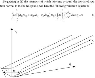
We consider the visco elastic waveguide as an infinite axial х1 variable thickness

(Figure 1). Basic relations of the classical theory of plates of variable thickness can be obtained on the basis of the principles of virtual displacements. The vari-ation equvari-ation problem visco elasticity theory in three-dimensional statement has the form

(

ij ij u ui i

)

d d dx x x3 2 1 0

(

i 1, 2, 3;j 1, 2, 3

)

ν

σ δε +ρ δ = = =

∫∫∫

(1)

where ρ-material density; ui-displacement components; σij and εij-components of

the stress tensor and strain; h-plate thickness; V-the volume occupied by the body. In accordance with the hypotheses of Kirchhoff-Love

(

)

12 23 33 0, i 3 , 3,

i

дw

u x w x t w

дx

σ =σ =σ = = − = _{. (2)}

Neglecting in (1) the members of which take into account the inertia of rota-tion normal to the middle plane, will have the following variarota-tion equarota-tion:

(

)

2

2 2

11 11 12 12 22 22 3 2 3

2 2

d 2 d d d 0

h h

S S

w

s x s w x

t

σ δε τ δε τ δε ρ δ

− −

∂

+ + + =

∂

[image:2.595.206.537.436.706.2]

∫ ∫

(3)

Based on the geometric relationships and relations of the generalized Hooke’s law, taking into account the kinematic hypotheses (2), the expressions for the

components of the strain and stress tensor has the form [7]

(

)

(

)

2

3

11 11 22 22 22 11 12 12

1

, , 1, 2; 2

; ; ,

1 1 1

j i ij

j i i j

u

u w

x i j

x x x x

E E E

ε

σ

ε

νε

σ

ε

νε

σ

ε

ν

∂ ∂  ∂ = _ + _− = ∂ ∂ ∂ ∂   = + = + = − − +

   (4)

( )

0

( )

(

) ( )

0

d , t

n n En

Eϕ t =E ϕ t − R t−τ ϕ t τ



∫



 ₍₅₎

where

ϕ

( )

t -arbitrary function of time; ν-Poisson’s ratio; REn

(

t−

τ

)

-the core

of relaxation; E01-instantaneous modulus of elasticity; we accept the integral

terms in (5) small, then the function ϕ

( )

_t =ψ

( )

_t e−iωRt, where

ψ

( )

_t -slowly

va-rying function of time, ωR-real constant. Then, we replace of (6) approximate

species [8]

( )

0 1

С S

n j j R j R

Eϕ=E _ − Γ ω − Γi ω _ϕ

where

( )

0

cos d

C

n ωR RЕn τ ω τ τR ∞

Γ =

_∫

_,

( )

0

sin d

S

n ωR RЕn τ ω τ τR ∞

Γ =

_∫

_{, respec-}

tively, cosine and sine Fourier transforms relaxation kernel material. As an ex-ample, the visco elastic material take three parametric relaxation nucleus

( )

1

e nt n

Еn n

R t =A −β t−α . Here An,α βn, n-parameters relaxation nucleus. On the

effect of the function RЕn

(

t−

τ

)

superimposed usual requirements inerrability,

continuity (except t=τ ), signs-certainty and monotony:

( )

0

d

0, 0, 0 d 1.

d

En

En En

R

R R t t

t

∞

> ≤ <

_∫

<

Introducing the notation for points

2 2 2 2

11 2 2 22 2 2

1 2 2 1

; ;

w w w w

М D v M D v

x x x x

∂ ∂  ∂ ∂  = _ + _ = _ + _

∂ ∂ ∂ ∂

   

(

)

2

₍

3

₎

12 2

1 2

1 , .

12 1

w Eh

M D v D

x x ν

∂

= − =

∂ ∂ −

When R_Еn

(

t−

τ

)

=0, then

(

)

3 2 12 1 Eh D ν =

− . Here E is the modulus of elas-

ticity.

Integrating (3) in the strip thickness leads to the following form

2 2 2 2

11 2 12 22 2 2

5 1 1 2 2

2 d d 0.

s

w w w w

M M M s h w s

x x

x x t

δ δ δ _ρ _δ

 ∂ ∂ ∂  ∂ + + − =   ∂ ∂ ∂ ∂ ∂  

∫

(6)

Integrating twice by parts and alignment to zero, the coefficients of variation

w

δ

inside the body and on its boundary and we obtain the following

(4)

(

)

2 2 2

2 2

11 12 22

2 2

1 2 2

2 0,

M M M

hw w w t

x x

x x ρ

∂ ∂ ∂

+ + + = = ∂ ∂

∂ ∂

∂ ∂   (7)

with natural boundary conditions:

2 2 2 0 0; 0; w x

w x l

∂  ₌ ∂   = =  (8) 1 1 1 0 0; 0; w x

w x l

∂  ₌ ∂   = =  (9)

The main alternative boundary conditions to them

22

22 12

2 2

2 1

0

2 0; 0;

M M M x l x x =   ∂ ∂  ₊ ₌ ₌  ∂ ∂  (10) 11 11 12 1 1 1 2 0

2 0; 0;

M M M x l x x =  _∂ _∂  ₊ ₌ ₌  ∂ ∂  (11)

For, we construct a spectral problem by entering the following change of va-riables 2 2 2 22 12 2 2 2 1 1 2 ; ; ; . W w W x M M W W M Q x x x x

ϕ

∂ = = ∂ ∂ ∂  ∂ ∂ = _∂ + _∂  = _∂ + _∂   (12)

Substituting (12) into (7) we obtain the differential equation of the system rel-atively sparse on the first derivatives х2 :

(

)

(

)

2 2 2

2 1 1

2 2 2 1 2 2 2 1 2 1 0; 1 0; 0; 0.

Q M W

D h

x x x t

M W

Q D

x x

W

D M D

x x W x ϕ ν ρ ν ϕ ϕ ∂ ₊∂ ₊ _′ ₋ ∂ ₊ ∂ ₌ ∂ ∂ ∂ ∂ ∂ _{− −} _′′ ₋ ∂ ₌ ∂ ∂ ∂ ∂ − + = ∂ ∂ ∂ _{− =} ∂ (13)

And alternative boundary conditions х2=0; x2=l2; 0

ϕ= or

(

)

22

1

1 M 0;

M D v

x

∂

− − =

∂

0 W

=

or

(

)

2 2 1

1 0.

Q D v

x

ϕ

∂

+ − =

∂ (14)

(5)

0

ϕ= or

(

)

22

1

1 M 0;

M D v

x

∂ − − =

∂

0 W

=

or

(

)

2 2 1

1 0

Q D v

x

ϕ

∂

+ − =

∂ (15)

Now consider the infinite along the axis х1 band with an arbitrary thickness

changes h=h x

( )

2 . We seek a solution of problem (13)-(15) in the for

(

_{Q M}_, _{, ,}ϕ_W

)

T=

(

_{Q M}_, _{, ,}ϕ _W

)

T_ei(αx1−ωt) (16)

Describing the harmonic plane waves propagating along the axis х1. Here

(

)

T

, , ,

Q M ϕ W -complex amplitude-function; k-wave number; С (С С= _R+iC_i)-

complex phase velocity; ω-complex frequency.

To clarify their physical meaning, consider two cases:

1) k=kR; С С= R+iCi, (ωR =ωI+iωI) then the solution of differential

Equations (13) has the form of a sine wave at х1, whose amplitude decays over

time;

2) k=kR+ikI; С С= R, Then at each point х1 fluctuations established, but х1

attenuated.

In both cases, the imaginary part kI or CI characterized by the intensity of the

dissipative processes. Substituting (16) in (17), we obtain a system of first order differential equations solved for the derivative

(

)

(

)

2 2 2

2

1 0;

1

0; 0

Q М D v h W

М Q D v W

M W

D W

α α ϕ ρ ω α

ϕ α

ϕ

′− − ′ − − = ′− + ′ − =

′ − − = ′ − =

(17)

with boundary conditions at the ends of the band х2 = 0, l2, one of the four types

1) Swivel bearing: W =M =0 (18)

2) Sliding clamp: Q= =

ϕ

0 (19)

3) Anchorage: W = =ϕ 0 (20)

4) Free edge:

(

)

(

)

2

1 0

M D W

Q D

α

ν

α

ν

ϕ

 + − = 



− − =

 (21)

Thus, the spectral formulated task (17) and (21) the parameter α2_{, describes}

the propagation of flexural waves in planar waveguide made as a band with an

arbitrary coordinate on the thickness change х2. It is shown that the spectral

para-meter α2_{It takes complex values (in the case of}

(

)

₀

Еn

R t−

τ

≠ ) If R_Еn

(

t−

τ

)

=0,

whereas the spectral parameter α2_{It takes only real values. Transform this}

sys-tem (17). We have

(

)

2

(

)

2

1 1

Q′=M′′+D′′ −v α W+D′ −v α ϕ

From whence

(

)

2 2 2

1 0

M′′+D′′ −v α W −α M −ρhw W=

(6)

2

1

0.

W M W

D

α

− − =

Thus, the conversion system is of the form

(

)

(

)

2 2 2

2

1 0

M M h D v W

W W M

D

α ρ ω α α  ′′− − − ′′ − =   ′′ − − =   (22)

The boundary conditions (18)-(21) in alternating W M, it has the form:

1) Swivel bearing: W =M =0; (23)

2) Sliding clamp: 2

(

)

1 0;

W′=M′−α D′ −ν W = (24)

3) Anchorage: W =W′=0 (25)

4) Free edge:

(

)

(

)

( )

2

1 0

M D W

M DW

α ν α ν ′ + − =

′

′ − − = (26)

at х2=0 or х2 = +l2.

Let М and W some own functions of the system (22)-(26) may have a

complex meaning. Multiply the equation system (22) to function _Mˆ _and_Wˆ _,

complex conjugate to М and W . Identical converting the first equation, we

integrate the resulting equality х2 and composed of the following linear

combi-nation

(

)

( )

(

)

( )

(

)

2 2 2

2 2

2 2 2

0 0 0

2 2 2

0 0 0

2

2 2 2

0 0 0

ˆ_d ₁ ˆ_d ₁ ˆ_d

ˆ_d ˆ_d ₁ ˆ_d

ˆ

ˆ_d ˆ_d _d ₀

l l l

M W x DW W x DW W x

MW x hWW x D WW x

MM

W M x WM x x

D

α ν α ν

α ω ρ α ν

α ′′ ′′ ′′ − − + − ′′ − − − − ′′ + − − =

∫

         (27)

Integrating (27) by parts,

(

)

(

)

(

)

(

)

(

)

(

)

(

)

2 2 2 2

2 2 2 ₂

2 2 2 2 0 ₀ 2 2 2 2 0 0 2 2

2 2 2

0

0 0 0

2 2 2

2 2

0 0

ˆ ˆ

1 d

ˆ

1 d d

ˆ

ˆ ˆ ˆ

2 1 d d d

ˆ ˆ

2 1 d 1 d 1

l l

l l l l

l l

M DW W M W M W x

DW W x MW MW x

MM

D WW x hWW x x W M

D

D W W x D WW x v D

α ν

α ν α

α ν ω ρ

α ν α ν α

   ′− − ′  − ′ ′+ ′ ′   _ _   ′ ′ ′ + − − _ + _   ′′ ′ + − − − + ′ ′ ′ ′ ′′ + − + − + −

∫

 _        

  2

2 0

ˆd 0 l

W W x =

∫

 or

(

)

( )

(

)

(

)

(

)

(

)

(

)

( )

2 2

2 2 2

2 2

0 0

2

2 2 2

0 0 0

2 2 2

0 0 0

ˆ ˆ ˆ

1 1

ˆ

ˆ ˆ _d ˆ ˆ _d _d

ˆ_d ₂ ₁ ˆ _d ₁ ˆ _d _0.

l _l

l l l

l e e

M v DW W M v DW W

MM

M W M W x WM WM x x

D

hWW x v D WW x v D WW x

α α

α

ω ρ α α

(7)

It is easy to make sure that is the integral terms of (28) vanish at any combina-tion of the boundary condicombina-tions (23)-(26). It should also be noted that all the functions under the integral valid at R_Еn

(

t−

τ

)

=0. The expressing α2 (28) We

find that

(

)

(

)

(

)

(

)

( )

2 2 2

2

2 2 2

2 0 0 0

2 2 2

0 0 0

ˆ

d d d

ˆ ˆ _d _{2 1} ˆ_d ₁ ˆ _d

l l l

MM

M W M W x x hWW x

D

MW MW x D WW x D WW x

ω ρ α ν ν ′ ′+ ′ ′ + + = ′ ′′ ′ + − − − −

∫

 _    

    -real

number.

Thus (with R_Еn

(

t−

τ

)

=0), It is shown that the square of the wave number

for own endless strip of varying thickness is valid for any combination of boun-dary conditions. If R_Еn

(

t−

τ

)

≠0, then α2_{It is a complex value for any} com-bination of boundary conditions.

3. Adjoin Spectral Problem, Orthogonality Condition

The resulting spectral problem (17)-(21) is not self-adjoin. Built for her adjoin

problem using this Lagrange formula [9]

( )

*

(

*

)

*

( )

*

0

0 0

d , d ,

l _l l

L U ⋅V x=Z U V − L V ⋅U x

∫

(29)

where L and L*—direct and adjoin linear differential operators; U and V*—arbitrary decisions of relevant boundary value problems.

In our case

(

)

(

)

2 2 2

2 2 2 2 2 2 1

1 0 1

1 0

0 0 1

д

D v h

дх д D v дх L д D дх д дх

α α ρ ω

α α  ₋ ₋ _′ ₋ ₋      ₋ ₋ _′ ₋    =    ₋       −      (30)

on the left-hand side of Equation (29) will be as follows

(

)

(

)

2

2 2 2

0

2 2

2

1 1

1 d 0

l

Q Q MQ D Q h WQ M M QM

D WM M W W W W x

D

α α ν ϕ ρ ω

α ν ϕ ϕ ϕ α ϕ ϕ

• • • • • • • • • • • •  ′ − − ′ − − + ′ −   ′ ′ ′ + − + − − + − _ =

∫

(31)

or, integrating parts

(

)

(

)

(

)

(

)

(

)

2 2 0 0 2 2

2 2 2

2

1

1 d 0

l l

QQ ММ WW Q M Q

M Q M W D Q

D

W D M h Q W x

ϕϕ

α ϕ ϕ α ν ϕ

α ϕ α ν ρ ω

(8)

Thus the conjugate (30)-(32), the system has the form

(

)

(

)

2

2 2 2

0 1 0 1 0 1 0 Q M M Q D

W D Q

W D M h Q

α ϕ

φ α ν

α ν α ϕ ρ ω

• • • • • • • • • • • •  ′ + =   _{′ +} ₊ ₌    ′+ + ′ − =   ′− ′ − + + =  (33)

Moreover, we get the conjugate boundary conditions of equality to zero is

integral members

(

_*

)

2

0

, l

Z U V expression in (32):

1) Swivel bearing:

ϕ

Q 0, x2 0,l2

•₌ •₌ ₌ ₍₃₄₎

2) Sliding clamp: W M 0, x2 0,l2

•₌ •₌ ₌

(35)

3) Anchorage: M Q 0, x2 0,l2

•₌ •₌ ₌ ₍₃₆₎

4) Free edge:

(

)

(

)

2

2 2

1 0,

1 0, 0,

D Q

W D M x l

ϕ

α

ν

α

ν

• • • •  + − =   − − = = 

For conditions biorthogonality solutions once again use the Lagrange formula (29) in the form

( )

(

)

2

0 0

d , ,

l _l

L U V• L V• • U x Z U V•

 +  =

 

∫

(37)

that leads to the consideration of the following integral

(

)

(

)

(

)

(

)

2

2 2 2

0 2 2 2 2 2 2 1 1 1 1 1 1 l

i j i i j i i j i j i j

i j i i j i j i j i i j

i j i j j i j i j i j i j

i j i j j i j j i i j

j i j j i

Q Q M Q D Q h W Q M M

Q M D W M M W

D

W W W Q Q M Q M M M Q

M W D Q W W

D

W D W

α α ν ϕ ρ ω

α ν ϕ ϕ ϕ α ϕ

ϕ α

ϕ ϕ ϕ ϕ α ν ϕ α ϕ α ν

• • • • • • • • • • • • • • • • • • • • • •  ′ − − ′ − − + ′  ′ ′ − + − + − − ′ ′ ′ + − + + + + ′ ′ ′ + + + + − + ′ + − −

∫

2 2 d 0,

j j i

M•+ρ ωh Q W• _ x =

(38)

where

(

)

T

, , ,

i i i i

Q M ϕ W -own form, corresponding to the Eigen value αi original

spectral problem;

(

Q Mj, j,

ϕ

j,Wj

)

T

• • • • _{-own form, corresponding to the Eigen}

value αj adjoin.

Integrating (38) by parts

(

)

(

)

(

)

(

)

(

)

2 2 2 2 2 0 0

1 1 d

1 1 0,

l

i j i j j i i j i j

l

j i i j

M Q D Q D W M W x

D Q D W M

α α ν ϕ ν ϕ

ν ϕ ν

• • • • • •  _  ′ ′ −  _− − − + − − _     +_ − − − _{ }=

∫

(39)

where to i≠ j we have the condition biorthogonality forms:

(

)

(

)

(

)

(

)

]

2 2 2 0 0

1 1 d

1

l

i i j i j j

l

i j j i ij

M D Q W D M x

D W M Q

ν ϕ ϕ ν

ν ϕ δ

(9)

The expression W Mi j Qjϕi

•₋ • _{zero, if the border is set to any of the}

condi-tions (18)-(21) in addition to the condicondi-tions of the free edge.

4. Fixed Problem for a Semi-Infinite Strip of Variable

Thickness

Consider a semi-infinite axial x1 lane variable section, wherein at the end (x1 = 0)

harmonic set time exposure of one of two types of:

( )

2 e , 11

( )

2 e , 0

i t i t

W W l

W = f x ω M = f x ω x = (41)

or

( )

1 2 e , 1 2 e , 1 0

i t i t

Q

fϕ x ω Q f x ω x

ϕ = = = ₍₄₂₎

where

(

)

3 3

1 1 3 2

1 1 1 2

, 2 1

W W W

Q D

x x x x

ϕ =∂ = _∂ + −ν ∂ _

∂ _∂ ∂ ∂ _ (43)

Transform the boundary conditions (41) so that they contain only selected our variables W, φ, M and Q

( )

2 22 22

( )

2 1

1 2

e ,i t e ,i t 0,

w M

W W

W f x D f x x

x x

ω ∂ _ν∂  ω

= _ + _= =

∂ ∂

 

( )

2 33

(

)

3 2

( )

2 1

1 1 1 2

e ,i t 2 1 Q e ,i t 0,

W W W

f x D f x x

x x x x

ω ω ϕ ν   ∂ ∂ ∂ = _ + − _= = ∂ _ ∂ ∂ ∂ _ or

( )

2 22 22

(

)

22

( )

2 1

1 2 2

e ,i t 1 e ,i t 0,

w M

W W W

W f x D D f x x

x x x

ω ∂ _ν∂  _ν ∂ ω

= _ + _− − = = ∂ ∂ ∂  

( )

(

)

( )

2 1

2 2 2

2 1

2 2 2

1 1 2 2 1

e ,

1 e , 0,

i t i t Q W f x x

W W W

D D f x x

x x x x x

ω ϕ ω ν ∂ ₌ ∂       ∂ ∂ ₊∂ ₊ ₋ ∂ ∂ ₌ ₌       ∂ __ _∂ ∂ ___ ∂ _∂ _ Of finally

( )

2 e ,

( )

2

(

1

) ( )

2 e , 1 0

i t i t

w M w

W = f x ω M =_f x +D −ν f′′ x _ ω x = (44)

( )

(

) ( )

2 1

2 2 1

1

e ,

1 e , 0.

i t i t Q W f x x M

f x D f x x

x ω ϕ ω ϕ ν ∂ = ∂ ∂ _ _′′ _ =_ − − _ = ∂ (45)

Assume that the desired solution of the no stationary problem can be ex-panded in a series in Eigen functions of the solution of the spectral problem. In the case of constant thickness it is evident, and in general, the question remains open.

(10)

( )

( 1 )

2 2

1 ₂

2

e k

k

N

k i x t

k

k _k

k

W W x

x a

M M x

Q Q x

α ω

ϕ ϕ ₋ ₋

=

 

 

=  

 

   

   

∑

. (46)

where W_k,

ϕ θ

_k, _k,M_k-biorthonormal own forms of the spectral problem (17) -

(21).

The representation (46) gives us the solution to the problem of non-stationary wave in the far field, i.e., where it has faded not propagating modes. The number of propagating modes used N course for each specific frequency ω, since the cu-toff frequency is greater than the other ω.

Consider two cases of excitation of stationary waves in the band: 1) fw=0-antisymmetric relative х1;

2) f_ϕ=0-symmetric.

In the case of antisymmetric excitation, substituting (46) into (44) and ex-pressing fM(x2), obtain

( )

2

( )

2

1

N

M k k

k

f x α M x

=

∑

. (47)

Value biorthogonality (40) gives expression to determine the unknown coeffi-

cients 2

( ) ( )

2 2 2

0

d e

k M k

a =

∫

f x Q• x x .

In the case of a symmetrical excitation fQ

( )

x2 We obtain rearranging (46)

to (45) in the following form

( )

2

(

( )

2

)

1

N

Q k k k

k

f x iα a M x

=

∑

− (48)

Biorthogonality ratio (30) gives

( )

2

2 2

0

d l

k Q k

k

i

a f x Q x

α

•

=

_∫

₍₄₉₎

Testing Software System and Study the Properties of

Propagation of Flexural Waves in a Band of Variable

Thickness

Testing program was carried out on the task of distributing the flexural waves in a plate of constant thickness. Consider the floor plate of constant thickness

infi-nitely satisfying Kirchhoff-Love hypotheses, with supported long edges (Figure

1).

At end face х1=0 specified:

( )

1 2 e , 11 2 2 e

i wt i wt

w= f x M = f x (50)

Spread along the axis х1 flexural wave is described by the differential control

(11)

(

)

2 2 2 2 1 2 2 1 0 0 , 0, 1 0 0, M

Q hw w w t

x M

w M

D x

w h h

ρ θ ϕ ϕ  _′ ∂ _′′ _′′ + + = = ∂ ∂  _∂  ′ − =   _∂  ′ − + =  _∂  ′− = =  (51)

with boundary conditions of the form (15)

(

)

22 2

1

0, 1 w 0, 0,π

w M D x

x

ν ∂

= − − = =

∂ (52)

Introducing the desired motion vector in the form of

( 1 )

ei a xk t

Q Q M M w W ω

ϕ

− −            _{ =}        _{  }     (53)

Go to the spectral problem

2 2 2 0, 0, 1 0, 0,

Q M hW

M Q

M W

D W

α ω ρ

ϕ α ϕ  ′ − − =  ′ − =   ′ − − =   ′  − =  (54)

with the boundary conditions

(

)

2

0, 1 0, 0,π

W= M+D −ν α W= x =

or

2

0, 0, 0,π

W= M= x = . (55)

Rewrite the system (54) as follows

2

2 2

1

0,

W M W

D

M M hW

α α ω ρ

 ′′− − =    ′′ − − =  (56)

and W=0, M=0, x2=0,π.

We seek the solution of (56) in the form

(

)

2

sin ,

sin , 1, 2, w

M

W a nx

M a nx n

=

= =  (57)

satisfying the boundary conditions (55).

We obtain an algebraic homogeneous system

2 2

2 2 2

1 0;

0.

W W M

M M w

n a a a

D

n a a ha

α

ω ρ

− − − =

− − − = (58)

(12)

2 2

2 2 2

1

detn D 0,

h n

α

ω ρ

α

+ = + or 2 2 1,2 , k h n D ρ

α + = ±ω _(59а)

where, when R_Еn

(

t−

τ

)

=0

2 2 1,2 . h n D ρ

α = − ±ω _(59b)

Ownership of constant thickness strip bending vibrations are of the form

1,2 2 1,2 2 1,2 2 1,2 2 sin ; sin ; cos ; cos . n n n n W nx

M hD nx

n nx

Q hD nx

ω ρ ϕ ω ρ = = ± = =_ (60)

We construct the solution of the problem adjoin to (54)-(55)

2 2 *

* 2 0, 0 1 0, 0

W h Q

W

M Q

D

Q M

α ϕ ρ ω ϕ ϕ α • • • • • • • •  ′ + + =   ′ + =   ′ + + =    ′ + =  (61) and * * 2

0, Q 0, x 0,π

ϕ

= = = _{. (62)}

Transforming (61)-(62) we obtain the following system of first order differen-tial equations 2 2 2 0 1 0, h Q Q Q D

ϕ α ϕ ρ ω α ϕ • • • • • •  ′′ − − =   ′′ − − =  

2 0,π; 0, 0.

x =

ϕ

•= Q•= (63)

The solution of (63) in the form

2 2

sin , Qsin

aϕ nx Q a nx

ϕ•₌ • •₌ • ₍₆₄₎

From whence 2

1,2

α It has the same form (59a), own forms of vibrations are of

the form: 1,2 2 1,2 2 1,2 2 1,2 2 sin , sin , cos cos . n n n n phD nx Q nx

W n phD nx

M n nx

(13)

For biorthogonality conditions direct solutions and the adjoin problem is ne-cessary to consider the following equation

π 2 2 0 2 2 2 2 2 1 1 d

i j i i j i j j i j i i j i j

j i j i j j i i j i j i i j j i

j i i j i j j i j i j i ij

Q Q M Q hW Q Q Q M Q M M Q M

M M M Q M M W

D D

W W W W W W W h Q W x

α ω ρ

ϕ α ϕ ϕ ϕ α ϕ ϕ ϕ

ϕ ϕ α ϕ ρ ω δ

• • • • • • • • • • • • • • • • • • • •  ′ − − + ′ + + ′ −  ′ ′ ′ + + + + − − +  ′ ′ + + − + + + = 

∫

(66)

where Q Mi, i,

ϕ

i,Wi-own form for the direct problem, the corresponding Eigen

values αi, and Q Mj, j,ϕj,Wj

• • • •_{-own form of the dual problem, the}

correspond-ing Eigen value αj. Integrating by parts in (66), using the boundary conditions

(55) and (62) we obtain the desired condition:

π

2 0

d

i j i j ij

M Q• Wϕ• x δ

 +  =

 

∫

. (67)

We now verify biorthogonality received their own forms (60) and (65) using the condition biorthogonality (67)

( )

( ) ( )

π

2 2 2 2 2

0

π

2 2 2

0

sin sin sin sin d

2 sin sin d π ij

hD ix jx hD ix jx x

hD ix jx x hD

ρ

ρ δ

 _⋅ ₊ 

 

= =

∫

The normalized adjoin eigenvector on π ρhD, we have a system of

eigen-vectors satisfying the condition (67).

We now obtain the solution of the problem of the distribution of the statio-nary wave in the semi-infinite strip of constant thickness. Suppose that at the border х1=0 set the following stationary disturbance:

( )

2

2 1

e sin e ,

e sin e , 0

i t i t

W

i t i t

M

w W b nx

M M b nx x

ω ω

= =

= = = (68)

We seek a solution of a problem

(

1 2

)

(

1 2

)

1 1

, , _k _k, , , _k _k

k k

w x x t a W M x x t a M

∞ ∞

= =

=

∑

=

∑

(69)

where

( )

_{( )}

( )

21 e , 2 e ,

k l k l

i a x t i a x t

k k

W =W x − −ω M =M x − −ω

а Wkи Mk-own form (60), corresponding to αk

It is evident from the band at the end face at x1=0 decision (69) must satisfy

the boundary conditions (68)

( )

2

( )

2

1

sin ei t ei t,

W k k

k

b nx ω a W x ω

∞

=

∑

( )

2

( )

2

1

sin ei t e ,i t

M k k

k

b nx ω a M x ω

∞

=

(14)

or go to the amplitude values

( )

2

1

sin ei t ,

w k k

k

b nx ω a W

∞

=

∑

( )

2

1

sin еi t ,

M k k

k

b nx ω a M

∞

=

∑

(70)

Consider the following integral

π π 2 2 1 1 0 0 π 2 1 0 d d d .

j j k k j k k j

k k

k k j k j j

k

MQ W x a M Q a W x

a M Q W x a

ϕ

∞ ∞ • • • • = = ∞ • • =    +  = _ + _   _ _   = _ + _ =

∑

∫

∑ ∫

(71)

On the other hand on the edge х1=0 the same integral as follows

( )

π

2 2 2

0

sin sin d

M j W j

b nx Q• b nx ϕ• x

 + 

 

∫

(72)

Substituting in (72) from the normalized own form (65) we obtain

( )

π

2 2 2 2 2

0

π

2 2 2

0

1

sin sin sin sin d

π π

sin sin d

π π

M w

w M

b nx jx b nx jx x

hD b b

nx jx x

hD ω ρ ω ρ   ±         = ± ⋅ ⋅    

∫

(73)

From a comparison of the formulas (71) and (73) it is clear that under such boundary conditions is excited only “n”-Single private form:

2 2 w M j nj b b a hD

ω

δ

ρ

±₌ _ _± _  

  (74)

Thus, the solution of the no stationary problem for a half-strip of constant thickness has the form

(

)

( )

(

)

( ) e e l l

i x t n n n n

W a W a W

M a M a M

α ω α ω − − + + − − − − − + − − = +

= + (75)

where

2

sin n

W±= ± nx , M_n±= ±ω ρhDsinnx₂ а an

±_{-determined from the ratio (74).}

Now suppose that the steady influence on the border of semi-infinite strip

1 0

х = _{it has the form}

( )

2 e ,

( )

2 e

i t i t

w M

w= f x ω M = f x ω (76)

Let us expand the function fw and fM Fourier series of sinus in the

inter-val

[ ]

0,π

( )

2

( )

2

( )

2

( )

2

1 1

sin , sin

k k

w w M M

k k

f x B kx f x b kx

∞ ∞

= =

=

∑

=

∑

(77)

(15)

(

)

( )

(

)

( )

1 1

e i xl t , e i xl t

k k k k k k k k

k k

W a W a W α ω M a M a M α ω

∞ ∞

− − − −

+ + − − + + − −

= =

=

∑

+ =

∑

+ (78)

where

2 2

k k

w M k

b b a

hD

ω ρ

±₌ _± _a

k

W±, Mk

±

determined from the ratio (60).

5. Numerical Results and Analysis

The numerical solution of spectral problems carried out by computer software

system based on the method of orthogonal shooting S. K. Godunov [10]

com-bined with the method of Muller. The results obtained in testing with the same software package analytically up to 4 - 5 mark frequency range from 0.01 to 100. Hereinafter, the entire analysis is conducted in dimensionless variables, in which

the density of the material ρ, half the width of the waveguide l2 and E modulus

taken to be unity, and the parameters of relaxation kernel

0, 048; 0, 05; 0,1

A= β = α= .

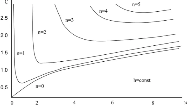
The calculation results are obtained when A = 0. Figure 2 shows the spectral

curves of the lower modes of oscillation of constant thickness plate, the corres-ponding n = 0, 1, 2, 3, 4, 5 for Poisson’s ratio υ = 0.25. Analysis of the data shows that the range of applicability of the theory of Kirchhoff-Love to a plate of con-stant thickness is limited by the low frequency range. For example, for the first

mode (h = 0), the range of application of the theory

0 ≤ ≤

ω

3

because of the

unlimited growth of the phase propagation velocity with increasing frequency,

for high frequencies C Cf s~ ω .

At high frequencies, where the wavelength is comparable or less than the fa-shion of strip thickness, there is, as is well known, localized in the faces of the

Rayleigh wave band at a speed slower speed Сs, however, as is obvious, this

[image:15.595.212.533.522.706.2]

for-mulation of the problem, in principle, does not allow to obtain this result. How-ever, it should be noted that in the application of the theory of Kirchhoff-Love platinum constant thickness is obtained the correct conclusion about the growth

(16)

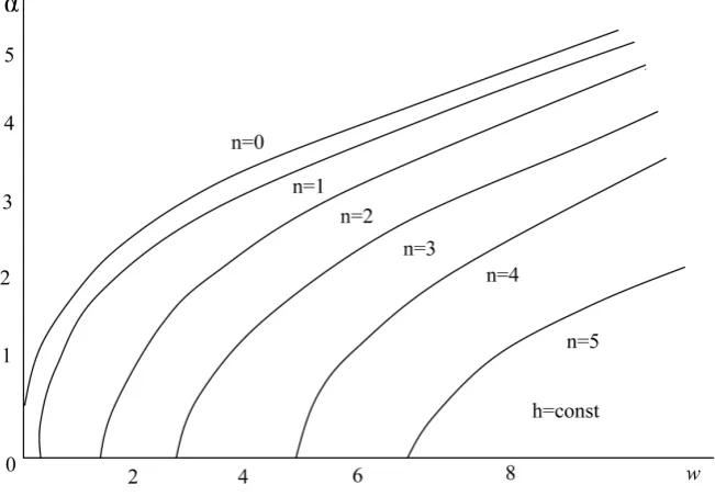
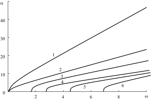
of the number of propagating modes with increasing frequency that is well seen

from the spectral curves of Figure 2 and Figure 3, which shows the dependence

of the wave number α the frequency for the same modes of waves.

Figure 4 shows the obtained numerical form for the above modes of oscilla-tions coincided with the same accuracy (4 - 5 decimal places) in the division of bandwidth by 90 equal segments.

[image:16.595.211.537.209.435.2] [image:16.595.214.539.462.709.2]

Figure 5 illustrates the solution of the stationary problem: the amplitude of the excited oscillation modes linearly depends on the frequency ω.

Figure 3. The dependence of the frequency of the wave.

(17)

We proceed to the propagation of flexural waves in a symmetric band Kir-chhoff-Love of variable thickness. Let us first consider a waveguide with a linear

thickness change, presented in Figure 6 and Figure 7 which are free edges.

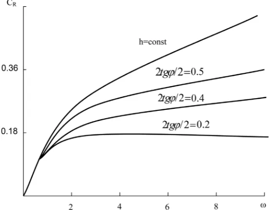
Fig-ure 8 shows the dispersion curves for the first mode, depending on the verge of tilt angle φ/2. Curve I corresponds to a strip of constant thickness h0=h1. Curve

2 corresponds to a waveguide with an angle of inclination of faces ϕ =2 π 4 or

tgϕ =2 1 and curve 3 corresponds to a waveguide tgϕ =2 0.2. The figure

[image:17.595.239.507.239.469.2]

shows that, unlike the bands in the case of constant cross-section of the wave-guide with a small tapered angle at the base of the wedge α (Curve 3) there exists a finite limit of the phase velocity of the fashion spread, and

Figure 5. The amplitude of the excited mode depending on the frequency.

[image:17.595.243.519.501.707.2]

(18)

[image:18.595.231.510.74.232.2]

Figure 7. The settlement scheme.

Figure 8. The dependence of the real and imaginary parts of the phase ve-locity on frequency.

lim 2 tg 2

f s

C C

ω

ϕ

→∞  =

where Сs-The speed of shear waves, which coincides with the results of other

studies [11] [12]. Thus, it is shown that-Lava Kirchhoff theory provides a wave

propagating in the waveguide is tapered with a sufficiently small angle at the base of the wedge-speed, lower shear wave velocity and different from the Ray-leigh wave velocity. Moreover, these waves from a frequency distributed without

dispersion. This wave is called “wave Troyanovskiy-Safarov” [13][14].

[image:18.595.236.514.272.488.2]

(19)

[image:19.595.233.519.68.268.2]

Figure 9. The forms of the coordinate fluctuations x2.

Kirchhoff theory-Lava applicability for studying wave propagation in wave-guides is tapered, as the frequency increases with decreasing length of one side of the wave modes, with different wave localizes with the sharp edge of the wedge so that the ratio of the wavelength and the effective thickness of the material is in the field of applicability of the theory [15]. This statement is true, the smaller the angle at the base of the wedge.

It should also be noted that the numerical analysis of the dispersion Equation (33) does not allow to show the presence of strictly limit the speed of wave propagation modes, since the computer cannot handle infinitely large quantities. We can only speak about the numerical stability result in a large frequency

range, which is confirmed by research. For example, when tgϕ =2 0.2 value

of the phase velocity of a measured without shear wave velocity at ω = 3 and ω = 40 It differs fifth sign that corresponds to the accuracy of calculations, resulting in test problem.

In the example h0 = 0.0001, it certainly gives an increase of the phase velocity

when the frequency increases further, since such a strong localization of the wave to the thin edge of the wedge, starts to affect the characteristic dimen-sion-the thickness of the truncated wedge, and Kirchhoff hypothesis-Lava stops working. To solve the problem of acute wedge numerically is not possible, since

the dispersion equation contains a term D−1_{, and the thickness tends to zero}

flexural rigidity D behaves as a cube and the thickness goes to zero. This signifi-cantly increases the “rigidity” (i.e. the ratio between the small and large coeffi-cient) system, increases dramatically the computing time and decreases the ac-curacy of the results. However, it is clear that you can trust the results obtained

where the agreed parameters h0 and α. We note also that the numerical

experi-ment showed no significant dependence of the phase velocity of the first mode of

the Poisson’s ratio ν, and the fact that a family of dispersion curves with

(20)

velocity to the limit does not depend on the angle of the wedge φ. On the modes, starting from the second, the speed limit dependence on Poisson’s ratio

be-comes noticeable about 8.5% for the second mode when changing

0 ≤ ≤

ν

0.5

.

[image:20.595.224.519.285.468.2]

Generally, the limit speed increases with the stronger and the more the mode number.

Figure 10 shows the dispersion curves for the first modal wedge

tgϕ =2 0.2. The figure shows that the speed of the first mode (curve I) is

equal to zero for ω = 0 and since the frequency ω = 1, virtually unchanged. The speed of the second mode (curve 2) is nonzero and finite for ω = 0 and stabilized at ω = 3. The rest of the modes (curve number matches the number of fashion)

have a cut-off frequency, which can be easily determined from Figure 11 (the

dependence of the wave number α of the frequency), and decreasing, stabilized (seen 3 and 4 modes) at top speed.

[image:20.595.227.527.512.709.2]

Figure 10. Dependence of the real and imaginary parts of the phase velocity on frequency.

(21)

[image:21.595.227.527.292.490.2]

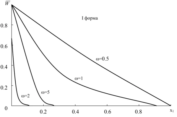
Figure 12 shows the evolution of the first waveform with the frequency ω for

frequencies ω = 0.5; 1; 5 и 20. Pronounced localized form with increasing

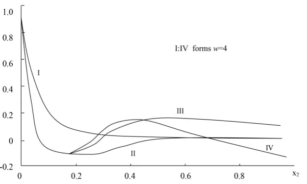
fre-quency. Figures 13-16 show the own forms respectively for 2 - 4 modes of

vi-bration for different frequencies: ω = 1, 2, 3 and 4 (the number of grid points corresponds to the number form). And here there are localized forms in the area

of thin wedge edge. Figure 16 gives an idea of the degree of localization of the

forms at the frequency ω = 1, obviously, the lower the number of forms, the

stronger it is localized at the edge of the wedge.

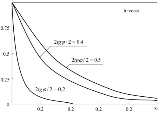
Figures 17-19 show the spectral curves of the first three events in the case of

the nonlinear dependence of the thickness of the strip from the coordinates х2.

( )

2 0 2, 0 2 1,

p

h x =h +hx <x ≤

where the parameter ρ It was assumed to be 1.5; 2; 2.5; 3 (curves 1, 2, 3, 4, re-spectively, curve “0” corresponds to p = 1-linear relationship).

[image:21.595.224.529.518.708.2]

Figure 12. Changing the shape of the coordinate fluctuations x1.

(22)

[image:22.595.225.521.71.291.2]

[image:22.595.230.517.320.500.2]

Figure 14. Changing the shape of the coordinate fluctuations.

Figure 15. Changing the shape of the coordinate fluctuations.

[image:22.595.228.529.529.709.2]

(23)

[image:23.595.237.508.69.260.2]

[image:23.595.241.504.292.482.2]

Figure 17. Changing the phase velocity as a function of frequency.

Figure 18. Changing the phase velocity as a function of frequency.

[image:23.595.242.505.517.708.2]

(24)

[image:24.595.232.517.75.259.2]

[image:24.595.234.519.290.478.2]

Figure 20. Change in the shape of the plate oscillations along the coordinate.

Figure 21. Change in the shape of the plate oscillations along the coordinate.

[image:24.595.232.518.513.710.2]

(25)

From the equation of “0” with the remaining curve shows that they are located on the horizontal high-frequency asymptote, monotonically to zero. The mi-drange is observed a characteristic peak which is shifted to lower frequencies

with an increase in “p”. In accordance with the charts of waveforms at Figures

20-22 quicker and localization of motion near the edge of the waveguide. Thus, it can be concluded that the phase velocity of the wave in the localized waveguide edge is defined as the frequency increases the rate of change of thick-ness in the vicinity of the sharp edge.

Figures 23-28 illustrate the solution of the stationary problem for a

wedge-shaped waveguide with a linear change in the thickness of the coordinates

[image:25.595.220.525.252.462.2]

х2 depending on the location of the excitation zone, from which it is clear that

[image:25.595.221.521.490.704.2]

Figure 23. The change factor а depending on the frequency.

(26)

[image:26.595.225.526.76.278.2]

the main contribution to the resulting solution brings a sharp edge excited

wa-veguides. Analysis of Figures 23-25 shows that, if aroused sharp edge of the

wedge is raised mostly first oscillation mode, and ratio α1 increases with

in-creasing frequency.

The amplitude of the remaining modes is not more than 5% from the first

(ω = 10). Upon excitation of the central waveguide portion (Figure 26 and

Fig-ure 27) the amplitude of oscillation is 20 - 50 times lower than when excited

sharp edge and decreases with increasing frequency. Figure 28 shows the factors

[image:26.595.222.525.306.523.2]

(27)

[image:27.595.224.531.64.274.2]

conclusion that in this case the entire frequency range can be divided into zones,

in which one of the modes propagates mainly. For example, in the case of Figure

25:

0 ≤ ω ≤ 2 I fashion; 2 ≤ ω ≤ 5 II fashion; 5 ≤ ω ≤ 10 III fashion, t. i.

6. Conclusions

[image:27.595.222.522.314.581.2]

(28)

- On the basis of the variation equations of the theory of elasticity, the

mathe-matical formulation of the problem of the propagation of longitudinal waves in plates of variable thickness is reduced to a system of differential equations with the corresponding boundary conditions.

- Showing that the square of the wave number for own endless bands of

varia-ble thickness in any combination of the action of the boundary conditions.

- The obtained spectral problem is not self-adjoint, so the associated problem

is constructed for it. Coupling system consists of ordinary differential equa-tions with the appropriate boundary condiequa-tions. With the help of the La-grange formula obtained conditions biorthogonality forms. The problem is solved numerically by the method of orthogonal shooting S. K. Godunov in conjunction with the method of Muller.

- Analysis of the data shows that the region with the imaginary theory of

Kir-chhoff-Love to the plate of constant thickness is limited by the low frequency range. At high frequencies, when wavelength comparable to fashion or less than the thickness of the plate, theory Kirchhoff-Love does not yield reliable results.

- For the phase velocity of propagation modes in the band of variable

thick-ness, there is final repartition unlike the constant cross-section strip.

References

[1] Bestuzheva, I.P. and Durov, V.N. (1981) On the Propagation of Edge Waves in Elastic Media. Akustik Journal, 27, 487-490.

[2] Bobrovnitsky, Y.I. (1977) Dispersion of Flexural Normal Waves in the Thin Strip. Akustik Journal, 23, 34-40.

[3] Skudrzyk, E. (1971) Simple and Complex Vibratory Systems. University Park and London, 558 р.

[4] Grinchenko, V.T. and Myaleshka, V.V. (1981) Harmonic Oscillations and Waves in Elastic Bodies. Kiev, 284 p.

[5] Kravchenko, V.T. and Myaleshka, V.V. (1981) Properties of Harmonic Waves Propagating along the Edges of the Rectangular Elastic Wedge. Akustik Journal, 27, 206-212.

[6] Meeker, T. and Metzler, A. (1966) Ducting in Long Cylinders and Plates. Def. Acoustics, Principles and Methods, Trans. from English, 1 A, 140-203.

[7] Koltunov, M.A. (1976) Creep and Relaxation. High School, Moscow, 273 p. [8] Rabotnov, Y.N. (1977) Hereditary Elements of Mechanics of Solids. Nauka,

Mos-cow, 384 p.

[9] Neumark, M.A. (1969) Linear Differential Operators. Nauka, Moscow, 526 p. [10] Mysovskikh, I.P. Lectures on Methods of Calculation: St. Petersburg University.

1998 p.

[11] Safarov, I.I., Teshaev, M.H. and Boltaev, Z.I. (2012) Wave Processes in the Mechan-ical Waveguide. Lambert Academic Publishing, Saarbrücken, 217 p.

[12] Safarov, I.I., Boltaev, Z.I. and Akhmedov, M.S. (2015) Distribution of the Natural Waves. Lambert Academic Publishing, Saarbrücken, 110 p.

(29)

with Attached Concentrated Mass. Lambert Academic Publishing, Saarbrücken, 92 p.

[14] Safarov, I.I., Akhmedov, M.S. and Boltayev, Z.I. (2015) Dissemination Sinusoidal Waves in of a Viscoelastic Strip. Global Journal of Science Frontier Research: F Mathematics and Decision Sciences, 15, 39-60.