Spatiotemporal Analysis and Predictive Modeling of Rabies in Tennessee

(1)

ISSN Online: 2151-1969 ISSN Print: 2151-1950

DOI: 10.4236/jgis.2018.101004 Feb. 7, 2018 89 Journal of Geographic Information System

Spatiotemporal Analysis and Predictive

Modeling of Rabies in Tennessee

Nyssa Hunt

1,2,3

, Andrew Carroll

2

, Thomas P. Wilson

1,3

1_{Department of Biology, Geology, and Environmental Science (BGES), University of Tennessee at Chattanooga, Chattanooga,}

Tennessee, USA

2_{Interdisciplinary Geospatial Technology Lab (IGTLab), University of Tennessee at Chattanooga, Chattanooga, Tennessee, USA} 3_{C/O Amphibian and Reptile Monitoring Initiative for a better Environment (ARMIE), Department of Biology, Geology, and}

Environmental Science (BGES), University of Tennessee at Chattanooga, Chattanooga, Tennessee, USA

Abstract

Among viruses, Rhabdovirus, more commonly known as rabies, is largely monitored throughout landscapes because of its known risks and deadliness. While vaccination and education efforts have been enforced and apparently successful in the past decades, many questions still exist in some regions about the virus’s spread and potential. In the United States, the state of Tennessee’s Department of Health has documented rabies reports from the 1940s-2010s, but not as many spatial analyses have been performed to further map and as-sess rabid animals in this variable landscape. Our study proposed to create distribution and density models to give an idea of the types of locations rabid animals have consistently been found. A predictive model was also created using software that simulated landscape fragmentation and habitat connectiv-ity, to provide further insight for potential disease spread. Our results display that Tennessee’s central region, which is a more homogenous landscape, tended to host a lot of rabid animals and maintained a rather consistent dis-tribution throughout the years. The predictive model was simulated on a less homogenous landscape and displayed that spread potential can be affected by natural barriers. Each of these spatial results could be of service in future dis-ease monitoring, hopefully for the benefit of wildlife and people alike.

Keywords

Epidemiology, Rabies, Predictive Modeling, Spatial Analysis, Habitat Connectivity

1. Introduction

Spatially and temporally, diseases have earned a noticeable level of recognition

How to cite this paper: Hunt, N., Carroll, A. and Wilson, T.P. (2018) Spatiotemporal Analysis and Predictive Modeling of Rabies in Tennessee. Journal of Geographic Infor- mation System, 10, 89-110.

https://doi.org/10.4236/jgis.2018.101004

Received: December 21, 2017 Accepted: February 4, 2018 Published: February 7, 2018

Copyright © 2018 by authors and Scientific Research Publishing Inc. This work is licensed under the Creative Commons Attribution-NonCommercial International License (CC BY-NC 4.0). http://creativecommons.org/licenses/by-nc/4.0/

(2)

DOI: 10.4236/jgis.2018.101004 90 Journal of Geographic Information System

attention to furthering research efforts. As with any virus, considering where ra-bies is still found, analyzing how fast it is spreading, and reflecting on prevention efforts can only expand on preexisting knowledge of this zoonotic disease.

Apart from Australia, Antarctica, and several island systems, rabies exists on a global scale [4] [5]. The virus itself is only found to exist in animals, primarily being terrestrial mammals and it thrives in this group [2] [6]. Furthermore, it is the class of mammals that might be considered of moderate size and appear to be most prominent. In the United States, these species include, but are not li-mited to: raccoons (Procyon lotor), skunks (Mephitis mephitis), bats (15 mem-bers of family Vespertilionidae), foxes (Urocyon cinereoargenteus and Vulpus vulpes), and coyotes/dogs (Canis latrans and Canis lupus familiaris) [3] [6]. Across the country, trends of host species have been observed for each region, consequently displaying broad distributions for the disease. Raccoons function as the main rabies reservoir along the Atlantic coast, while skunks and foxes are the main groups toward the west; the northernmost range (approximately up to 71˚N) exists in Alaska with foxes [6]. While the virus is rather widespread, though, its absence of information in certain sections of the west and of the southeast can lead to questions of what is necessary for it to abide in existing lo-cations.

(3)

As rabies continues to exist in various geographies, further studies have been performed worldwide to observe and predict its capabilities and impacts. In China, the virus was observed to begin in 139 counties in 2000; seven years later, that number increased to 980 counties, encompassing most of China’s more de-veloped region [7]. Similarly, the Indonesian archipelago has observed an emer-gence throughout the islands, as they gathered reports from each region using GPS points and GIS tools [8]. In Greece, a rabies outbreak was documented during 2012-2014, where certain agricultural landscapes were noted to facilitate rabid wildlife movement [9]. Studies in each of these regions display that the vi-rus functions throughout island nations as well as homogenous landscapes.

Within the United States, other levels of research have taken place in regard to modelling network activity and predictions [4] [10]. Connecticut has performed network studies, analyzing the speed of spread of rabies throughout the state and what paths of travel it has taken [11]. In Wyoming, spatial and temporal patterns of how a rabid raccoon might travel across the landscape have been predicted

[12]. Northern Texas has sought to create a simple rabies model for interactions between skunks and bats, which are two prominent rabies vectors in the state

[13]. Those cases represent a few forms of recent research efforts toward possible solutions, while influencing future ideas to expand upon.

2. Justifying Tennessee’s Need for Rabies Monitoring

As more is discovered of the rabies virus, new questions and research opportuni-ties arise, especially for areas of the country that receive a lesser amount of atten-tion. Specifically, the southeastern section of Tennessee has not posted any pub-lic updates regarding what the spread status of rabies is now, while citizens are commonly wary. Vaccination efforts and prevention methods via bait have been reported successful in recent decades, but this still leaves questions as to whether the virus is totally eradicated or is still a cause of concern [3]. In truth, the virus may have spread to unknown and unmonitored locations, or perhaps the data has yet to be released to the public. Some agencies from which to gather rabies data include the CDC, the US Department of Agriculture (USDA), the US De-partment of Health and Human Services (USDHHS), and Tennessee Wildlife Resources Agency (TWRA), as each gain records of cases reported in certain re-gions [3]. But again, not all regions receive the same amount of surveillance and therefore would result in data gaps.

Because of the many questions rabies poses in Tennessee (see Figure 1), we are driven to perform spatial analysis and modeling of the rabies virus distribu-tion for both the state and southeastern Tennessee region. Analyzing historic and present data allows a spatiotemporal view on disease spread to better eluci-date areas of concern. Not only does this have the potential to reveal the capacity of rabies presence in this section of the country, but it could also provide insight on future plans of action in combating the virus [10].

(4)

[image:4.595.120.540.61.260.2]

Figure 1. The region of interest, Tennessee, highlighted in blue and showcasing the broadness of the area.

southeastern Tennessee and Appalachian region requires special attention to as-sess the landscape for natural barriers or corridors of travel [10] [14]. In contrast to states like Kansas or Oklahoma, which are more prairie-like, eastern Tennes-see contains a ridge and valley system that produces a much different arena for the wildlife. The significance of this lies with the type of area to be analyzed, as the region’s potential for disease facilitation has been previously understudied.

In conjunction with recorded GPS points, including some ecological data, such as the National Land Cover Dataset (NLCD) 2011, would be appropriate to extrapolate what areas rabies seems to “prefer most”. Along with this, a habitat connectivity model could also reveal correlation between habitat types and “dis-ease corridors”, where NLCD data will be necessary [10] [14]. However, a level of bias must be considered, as the virus would have had to have been observed by humans and with some proximity to developed areas. One might question – is it possible to accurately map where rabies resides most and predict its spread from there? Therefore, we hypothesize that using habitat connectivity modeling will provide a new aspect of disease monitoring and prediction of the rabies vi-rus distribution.

3. Materials and Methods

3.1. Hardware and Software Requirements

(5)

guide, at least 2 gigabytes of RAM are required to handle simple tasks, though insufficient RAM is the most common cause of program failure [16]. Similarly, Fragstats requires 2 gigabytes of RAM at minimum, but a computer having at least 4 gigabytes is preferable [15]. With these aspects in mind, a computer with 8 GB of RAM, an i5 Intel Core processor, and approximately 250 GB of hard drive space was used for this project, as those specifications were adequate to ba-sic memory and processing requirements.

3.2. Rabies Occurrence Data Acquisition

and Initial Data Processing

To begin, GPS points of documented rabies cases were sought after from a couple of health agencies. First to be contacted was the CDC; however, the data they possessed could not be shared. Second, the Tennessee Department of Health (TDH) was contacted and point data was successfully acquired. The agency also included a file that contained all counties of Tennessee and rabies information for each county, which assisted in referencing all points to their locations. Fur-thermore, the points ranged back to 1942, which would allow for a great amount of historical analysis. With these pieces of data in possession, it would now be possible to analyze temporal ranges and densities throughout the state and over time [1].

However, while the point data included 12, 889 reported cases of animal ra-bies, ranging from 1942-2014 by county, the points were programmed to be randomly generated in their respective counties. This presented a shift in the ul-timate direction and broadened some focuses, but still allowed for general spatial processing.

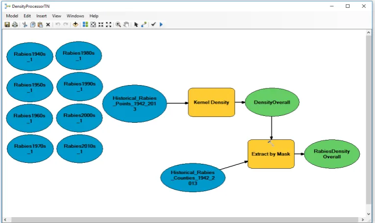
As the amount of cases was so large, it was appropriate to break them up by time eras; the entire point shapefile was split into decades by repeatedly selecting attribute and exporting the selections to separate files. Thus, standalone files for the 1940s, 1950s, 1960s, etc. could then be viewed and finer details could be made out over time. From those files, polygons were generated for each decade era to define the basic range of the rabies virus within Tennessee. A model was created to efficiently create each of these ranges, which input a point shapefile, converted them to a series of lines, and then converted the final output into a polygon (see Figure 2). Each of these range polygons were stored in a feature dataset, which was also contained in a file geodatabase created to store the gen-erated files in this project.

Following the creation of general ranges, temporal densities with each decade were sought to be processed. By viewing the points alone, it was evident that certain counties contained clusters of points, displaying concentrations of re-ported rabies cases. Another model was created for each point file to be processed with the Kernel Density tool, which calculates the amount of concentra-tion of points within an area and considers the proximity of the points (see

(6)

[image:6.595.107.492.74.403.2]

Figure 2. An ArcGIS workflow built for creating rabies distribution polygons for each decade, utilizing tools that convert the

ra-bies presence points to lines, converting lines to polygons, and lastly dissolving lines in the polygon to produce a continuous po-lygon representing geographic distribution.

Figure 3. An ArcGIS workflow built to process rabies density models throughout the decades, where rabies points are processed

[image:6.595.108.491.463.691.2]

(7)

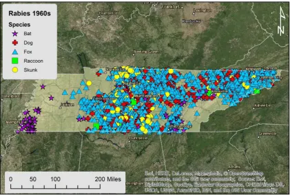
Along with general density, the prevalence of certain species throughout the areas was noticed, thus brought the need to highlight these species for each dec-ade: Dog, Fox, and Skunk. Two other species of concern were also considered: Bat and Raccoon. A visual for each era was created, with only the specified ani-mals included on the legend (if present in the decade), and exported.

3.3. Data Preparation for Predictive Modeling

The Memphis, Nashville, Chattanooga, Knoxville, and Tri-Cities areas were found to contain high concentrations of rabies cases, as was evident from the cumula-tive density layer. Therefore, the counties with the highest concentrations of ra-bies were selected and set aside for clipping, due to the apparent significance in cases. Perhaps the greatest question at this point is: what habitats are hosting ra-bid animals?

Acquiring the NLCD data from the government posted site was the next step in finding an answer to this question. Though the 2011 dataset was initially thought to be needed, the 2000s era was more complete as a decade in its docu-mentation of rabies cases. Knowing this, NLCD 2001 was selected for its spati-otemporal relevancy to the 2000s era rabies cases documented, also being rele-vant for simulating distribution trajectory. This data was found to be rendered in the same resolution as NLCD 2011.

The NLCD 2001 data was downloaded and uploaded onto ArcMap, which was soon after clipped to the defined counties from earlier. Doing this revealed that while deciduous forest was the most dominant land cover type of all the coun-ties, the areas that experienced incredibly high concentrations also contained noticeable proportions of impervious surfaces and hay/pasture lands. Based on the trends of impervious surfaces and hay/pasture lands, along with the known ecology of wildlife known to utilize those lands, these areas were selected as the habitat types for modeling connectivity.

3.4. Spatial Analysis with Fragstats and Circuitscape

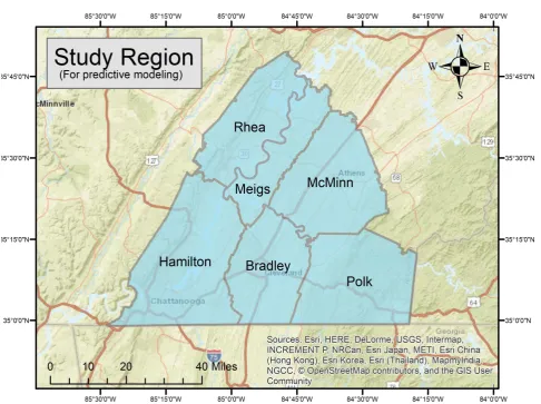
The Chattanooga area and five other southeastern Tennessee counties were tar-geted for the predictive modeling, for the sake of time potentially required for the process and computational capability. Outside of Hamilton county, the fol-lowing counties were selected: Bradley, Polk, Rhea, Meigs, and McMinn (see

Figure 4). These counties are directly to the north and east of Hamilton, and

have also displayed some cases for rabies in the 2000s. From the counties shape-file provided by the TDH, these 6 counties were selected and exported to become a separate file. From there, this new boundary allowed for an extraction of the NLCD 2001 by using the Extract by Mask tool for the raster.

Fragstats is a program that specializes in identifying habitat fragmentation and ranking habitat patches according to quality based on the geometry of each

area [15]. Running this tool will yield an output file that can be used to process

(8)

[image:8.595.57.544.61.424.2]

Figure 4. The study region chosen for predictive modeling, which includes the Tennessee counties of Hamilton, Rhea, Meigs,

Bradley, McMinn, and Polk, all of which are in the southeastern area of the state.

clipped NLCD had to be converted into a binary format for it to be able to frag-ment the landscape into patches. This was done by performing a series of reclas-sifications using the Reclassify tool in ArcGIS, in which the hay/pasture and im-pervious surfaces were reclassified to 1 and all other surfaces were reclassified to 0, indicating areas where the surfaces of interest are absent. Because the NLCD does not include road surfaces, those also had to be added using the Raster Cal-culator tool and the subsequent file experienced another reclassification. After these steps, the file needed to be converted into ASCII format, as this file type consistently runs successfully on Fragstats.

(9)

Following this, another reclassification was performed to separate the values into 10 categories in this case, 1 being the “best for spread” and 10 being the “worst for spread”.

In order to execute Circuitscape [16], the program that is used to model con-nectivity over a landscape, two files are needed: one to represent focal nodes, which highlight areas of interest to solve connection combinations for, and one to represent the resistance/conductance, on which the program will attempt to solve for each of the focal nodes. The Core Area Index (CAI) file that resulted from Fragstats was converted to ASCII to function as the resistance/conductance. As for the nodes, some of the existing rabies points were used as a simulation for this predictive model. As 30 connectivity pairs would be needed for a sufficient sample, 11 nodes were created (one extra in case a node drops out); these nodes were converted from point to raster, then raster to ASCII. Another key aspect to note is that these ASCII files must be in the same resolution and extent in order to run together [16]. The pixel resolution for these files had to be shifted to ap-proximately 40 m during all of the conversions, which proved to be fine enough to make out details, while coarse enough for the computer to handle processing.

4. Results

Each phase of the spatial analysis was built on previous modeling steps: the dis-tribution models revealed the occurrence history, the cumulative density re-vealed which land features may have been exploited by primary carriers of ra-bies, and the habitat connectivity modelling simulated how certain landscapes could facilitate disease spread. The graphics highlighted in the following sections are a testament to each of these aspects.

4.1. Distribution Models

(10)

[image:10.595.73.527.76.249.2]

Figure 5. This polygon represents the rabies range of occurrence during the 1940s, where the range is observed to cover most of

[image:10.595.76.522.296.470.2]

Tennessee.

Figure 6. During the 1950s, the range for rabies in Tennessee was slightly retracted in the northwest, but still rather broad

throughout the state.

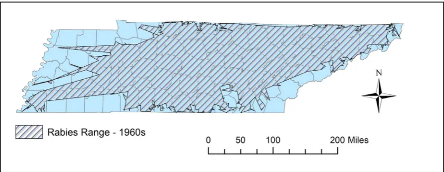
Figure 7. While rabies distribution was broad in the central and eastern regions of Tennessee during the 1960s, western

[image:10.595.74.522.515.689.2]

(11)

[image:11.595.67.531.73.252.2]

Figure 8. In the 1970s, the rabies reports in the west decreased, while the central and northeastern regions displayed solid

[image:11.595.70.529.296.474.2]

preva-lence, as reflected by this polygon.

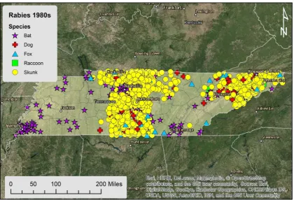
Figure 9. In the 1980s, the western rabies distribution expanded again, while being solid in the central and eastern regions.

Figure 10. In the 1990s, some sections of southeastern Tennessee experienced retractions in distribution, while the west began

[image:11.595.75.530.512.690.2]

(12)

[image:12.595.75.526.70.244.2]

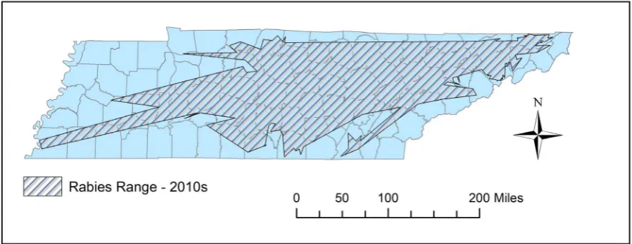
Figure 11. By the 2000s, rabies distribution became broadened to most regions of the state, while not being present as much in the

northwestern area.

Figure 12. This polygon is reflective of rabies cases documented up to 2014, which makes the 2010s an incomplete dataset. Still, a

retraction of cases in the west and southeast is noticeable, with areas in the central and northeast regions still having solid pres-ence.

4.2. Density Models

Performing a kernel density of all rabies cases in Tennessee revealed high con-centrations in certain counties and regions of the state (see Figure 13). Shelby county displayed the most density in western Tennessee; Davidson, Williamson, Rutherford, Maury, Wilson, Robertson, and Sumner counties displayed the most density in central Tennessee; Hamilton county displayed the most density in southeastern Tennessee; Knox, Washington, and Sullivan counties displayed the most density in northeastern Tennessee.

[image:12.595.77.520.295.466.2]

(13)

cases of bats also being reported in various parts of the state (see Figures 16-19). In the 2000s, raccoons were reported with rabies for the first time in Tennessee, occurring in the eastern region of the state (see Figure 20). By the 2010s, rabies cases have the appearance of decreasing in case count, but the amount of skunks reported is still of concern (see Figure 21).

[image:13.595.208.540.170.418.2]

Overall, the densities of cases displayed which areas received the most rabies

Figure 13. A cumulative density map of the rabies cases reported in Tennessee, from the

1940s-2010s; highly populated regions were noted to have had some of the highest densi-ties of rabies reports.

Figure 14. Throughout the 1940s, dogs accounted for 2145 out of 2442 rabies reports

[image:13.595.210.541.472.691.2]

(14)

[image:14.595.85.513.72.350.2]

Figure 15. Throughout the 1950s, dogs accounted for 1327 out of 2456 rabies reports total, indicating a rabies decline for that

species, while reports for foxes grew to 633.

Figure 16. Throughout the 1960s, rabies cases in foxes grew significantly, accounting for 1966 out of 3294 cases total, while dog

[image:14.595.89.511.394.677.2]

(15)

[image:15.595.84.514.69.351.2]

Figure 17. In contrast to the 1960s, the 1970s cases were split in dominance between skunks and foxes, where skunks accounted

for 394 out of 944 cases total and fox cases declined significantly to 271. Bat cases increased somewhat in western and eastern re-gions.

Figure 18. In the 1980s, skunks became the dominant reservoir species of rabies in central and northeastern Tennessee, accounting

[image:15.595.89.510.407.693.2]

(16)

[image:16.595.86.519.69.357.2]

Figure 19. Throughout the 1990s, skunk cases had decreased, but still remained the dominant rabies reservoir with 792 out of 965

cases total. Bat cases also declined to 87, though the cases began occurring more widespread in eastern regions.

Figure 20. In the 2000s, skunks were still the dominant rabies reservoir, with 689 out of 1011 cases total. Unlike previous decades,

[image:16.595.81.518.401.689.2]

(17)

[image:17.595.112.487.68.320.2]

Figure 21. Thus far into the 2010s, skunks are still dominant in terms of being rabies carriers, but now only account for 153 out of

229 cases total, which is a great drop compared to decades prior. Bats cases number to 39, while raccoons are at 8, which may be reflective of rabies vaccination programs.

Figure 22. Overall, from the years of 1942-2014, the total numbers of rabies cases in the five animals of concern are as follows:

Bat: 614; Dog: 3943; Fox: 2990; Raccoon: 105; Skunk: 3663 cases. Dog cases, represented in orange, have an obvious spike and de-crease from the 1940s-1960s. Fox cases, represented by the silver bar, display growth and a spike in the 1950s-1960s, also dwin-dling down in later decades. From the 1960s-2010s, skunks and bats, represented by dark blue and magenta respectively, have been steadily documented, with a spike in the 1980s for skunks and a slow decrease. Raccoons, represented in yellow, accounted for the least amount of rabies cases throughout the decades.

[image:17.595.99.499.377.587.2]

(18)

[image:18.595.208.540.248.674.2]

fragment spread potential [14] [20].

Figure 23. CircuitScape connectivity model: red areas indicate high levels of habitat

(19)

5. Discussion and Conclusions

Expanding on pre-existing knowledge provided by health agencies and replicat-ing predictive methods from similar research can hopefully give us a better idea on how to handle viral epidemics. Relating spread to a landscape, as this study was specialized for, can also allow insight into spatial thinking, which is an as-pect that should more often be considered with disease studies. The CDC, TWRA, USDA, TDH, and other related agencies would be able to use this information to add to their databases and to possibly enhance prevention strategies for rabies.

The spatial modeling methods performed in this study may reveal which sce-narios could be more efficient for rabies monitoring and mapping. The polygon ranges displayed very broad coverage, but may not represent the true range of rabies in the state as finely as the density maps. At the same time, the density maps are dependent on point data coming from consistent reports throughout the years. If rabies reports were not consistently given, hotspots may be biased to certain areas, such as those with high population densities. Both methods are able to give visual representation of basic presence, however, largely differing in broadness of coverage and spatial resolution.

Throughout the decades, certain groups of animals were documented in large numbers, seeming to occur in waves. The fact that dogs were documented with rabies most in the 1940s-1950s could be attributed to less vaccination strategies in place during the time period or simply less documentation of rabid wildlife during that era (Figure 14 and Figure 15). Dog cases decreased dramatically by the 1960s, while fox cases began occurring at a greater scale during that same decade, where central Tennessee’s more homogenous landscape might have faci-litated the spread more (Figure 16). In the remaining decades and up to the present, skunks took the place of foxes in terms of high rabies counts within the same regions of the state (Figures 17-20). These trends in rabid wildlife and where these waves occurred allow for speculation of what regions should be con-sidered for further spatial analysis and consideration of landscape ecology.

Predictive modeling is often an experimental frontier, though it continues to be of great use in spatial studies. Connectivity models can display habitat corri-dors that may not be noticeable at a glance and can give quick indications of which areas need to be monitored more closely. The output from Circuitscape

[16] in this study (Figure 23) displayed generally broad potential for infected animals to spread throughout the landscape, but the variation in landscape seemed to break higher potential in many areas [4] [11]. This observation may explain why the southeastern region of Tennessee may not have experienced as high of a rabies outbreak over the years, as non-homogenous landscapes can create landscape barriers to infected animals [20].

(20)

agnose rabies may have also had influence. This study’s main focus was to assess rabies occurrence based on available data, which unexpectedly unveiled trends in data occurrence need to be studied further.

This research created distribution and density summaries of documented ra-bies occurrence in Tennessee, which was previously understudied for decades in this area. The predictive aspects tested methods for mapping disease potential and habitat connectivity throughout unique landscapes of Tennessee. In addi-tion, the aforementioned models can identify other areas needing rabies moni-toring in the state. As shown in this study, continuous monimoni-toring and model creation of this virus, along with utilization of landscape analysis software, can assist in spatial reasoning for future vigilance.

Acknowledgements

This manuscript is based on an undergraduate capstone experience submitted by the first author (NH) in partial-fulfillment for the requirements set by the third author (TPW) for ESC 4920 (Advanced Applications of Remote Sensing and Geographic Information Systems in 2014). We gratefully acknowledge the Ten-nessee Department of Health for their contribution of data necessary for this project. We also thank the UT-Chattanooga Biology, Geology, and Environmen- tal Science Department for their support. Additionally, we thank the GIS lab for providing the resources and equipment required completing this process, as well as facilitating a fruitful and supportive learning environment with its personnel.

References

[1] Banyard, A.C., Horton, D.L., Freuling, C., Müller, T. and Fooks, A.R. (2013) Con-trol and Prevention of Canine Rabies: The Need for Building Laboratory-Based Sur- veillance Capacity. AntiviralResearch, 98, 357-364.

https://doi.org/10.1016/j.antiviral.2013.04.004

[2] The Humane Society of the United States (2017) Understanding Rabies—Facts and Safety Guidelines Clear Up Misperceptions.

http://www.humanesociety.org/animals/resources/facts/rabies.html?credit=web_id8 8988707#Which_Species_Carry_Rabies

[3] Tennessee Department of Health (2017) Rabies Control Manual 2017.

(21)

17.pdf

[4] Smith, D.L., Lucey, B., Waller, L.A., Childs, J.E. and Real, L.A. (2002) Predicting the Spatial Dynamics of Rabies Epidemics on Heterogeneous Landscapes. Proceedings of the National Academy of Sciences, 99, 3668-3672.

https://doi.org/10.1073/pnas.042400799

[5] Jackson, A.C. (2011) Research Advances in Rabies. Elsevier/Academic, Amsterdam. [6] Centers for Disease Control and Prevention (2017) Rabies.

http://www.cdc.gov/rabies/index.html

[7] Jinning, Y., Li, H., Tang, Q., Rayner, S., Han, N., Guo, Z., Liu, H., Adams, J., Fang, W., Tao, X., Wang, S., Liang, G. and Sá Carvalho, M. (2012) The Spatial and Tem-poral Dynamics of Rabies in China. PLoS Neglected Tropical Diseases, 6, e1640. https://doi.org/10.1371/journal.pntd.0001640

[8] Ward, M.P. (2014) Rabies in the Dutch East Indies a Century Ago—A Spatio-Tem- poral Case Study in Disease Emergence. Preventative Veterinary Medicine, 114, 11-

20. https://doi.org/10.1016/j.prevetmed.2014.01.009

[9] Giannakopoulos, A., Valiakos, G., Papaspyropoulos, K., Dougas, G., Korou, L.M., Tasioudi, K.E., Fthenakis, G.C., Hutchings, M.R., Kaimaras, D., Tsokana, C.N. and Iliadou, P. (2016) Rabies Outbreak in Greece during 2012-2014: Use of Geographi-cal Information System for Analysis, Risk Assessment and Control. Epidemiology &

Infection, 144, 3068-3079. https://doi.org/10.1017/S0950268816001527

[10] Wheeler, D.C. and Waller, L.A. (2008) Mountains, Valleys, and Rivers: The Trans-mission of Raccoon Rabies over a Heterogeneous Landscape. Journal of Agricultur-al, Biological, and Environmental Statistics, 13, 388.

https://doi.org/10.1198/108571108X383483

[11] Smith, D.L., Waller, L.A., Russell, C.A., Childs, J.E. and Real, L.A. (2005) Assessing the Role of Long-Distance Translocation and Spatial Heterogeneity in the Raccoon Rabies Epidemic in Connecticut. Preventive Veterinary Medicine, 71, 225-240. https://doi.org/10.1016/j.prevetmed.2005.07.009

[12] Ramey, C.A., Mills, K.W., Fischer, J.W., Mclean, R.G., Fagerstone, K.A. and Enge-man, R.M. (2013) Graphically Characterizing the Movement of a Rabid Striped Skunk Epizootic across the Landscape in Northwestern Wyoming. EcoHealth, 10, 246-256. https://doi.org/10.1007/s10393-013-0853-3

[13] Borchering, R.K., Liu, H., Steinhaus, M.C., Gardner, C.L. and Kuang, Y. (2012) A Simple Spatiotemporal Rabies Model for Skunk and Bat Interaction in Northeast Texas. Journal of Theoretical Biology, 314, 16-22.

https://doi.org/10.1016/j.jtbi.2012.08.033

[14] Rees, E.E., Pond, B.A., Cullingham, C.I., Tinline, R., Ball, D., Kyle, C.J. and White, B.N. (2008) Assessing a Landscape Barrier Using Genetic Simulation Modelling: Implications for Raccoon Rabies Management. Preventive Veterinary Medicine, 86, 107-123. https://doi.org/10.1016/j.prevetmed.2008.03.007

[15] McGarigal, K. (2012) FRAGSTATS v4: Spatial Pattern Analysis Program for Cate-gorical and Continuous Maps. University of Massachusetts, Amherst, MA. http://www.umass.edu/landeco/research/fragstats/fragstats.html

[16] McRae, B.H. and Shah, V.B. (2009) Circuitscape User’s Guide. The University of California, Santa Barbara, CA.

http://docs.circuitscape.org/circuitscape_4_0_user_guide.html

[17] Kramer, L. and Elliott, M. (2005) Identification of Conservation Opportunity Areas in Georgia. Gap Analysis Bulletin, 13, 14-20.

(22)

DOI: 10.4236/jgis.2018.101004 110 Journal of Geographic Information System (2006) Development of a GIS-Based, Real-Time Internet Mapping Tool for Rabies Surveillance. International Journal of Health Geographics, 5, 47.