Meta Heuristic Algorithm based on Ant Colony Optimization Algorithm, Tabu Search and Project Scheduling Problem (PSP) for the Traveling Salesman Problem

Received Nov 20, 2013 / Accepted Dec 19, 2013

Editorial Académica Dragón Azteca (EDITADA.ORG)

Meta-Heuristic Algorithm based on Ant Colony Optimization Algorithm,

Tabu Search and Project Scheduling Problem (PSP) for the Traveling

Salesman Problem

Fuentes-Penna Alejandro

_{, Estrada-Carrillo Marisa}

_{, Flores-Jiménez Ivette}

_,

Flores-Jiménez Ruth

and Moreno-Gutiérrez Silvia S.

1

_{Escuela Superior de Tlahuelilpan – Universidad Autónoma del Estado de Hidalgo}

_{Universidad Politécnica del Estado de Morelos}

1

_{alexfp10hotmail.com}

Abstract.

Keywords: Tabu Search, Project Scheduling Problem, Ant Colony Optimization, Traveling Salesman Problem.

1 Introduction

1.1 Tabu Search

Glover [33] describes Tabu Search as “a general heuristic procedure for guiding search to obtain good solutions in

complex solution spaces. Its rules are sufficiently broad that it is often used to direct the operations of other heuristic procedures”.

Hertz and de Werra [32] describes Tabu Search Method a: the search from an initial feasible solution s moving step by step defining a neighbourhood N of each point s* towards a solution giving the minimum value of some objective function, the next s* selection depends if f(s*) is better than f(s) or not.

Glover [33] proposed a Tabu Search Algorithm: Choose an initial solution s in X

stop: = false Repeat

Generate a sample V* of solutions in N(s).

Find a best s' in V* (i.e. f(s') < f(Y) for any ~ in V*). iff(s') >f(s) then stop: = true

else s := s' Until stop

Whei-Min et al [34] proposed the tabu restrictions when certain conditions imposed on moves, which make some of them forbidden, creating a tabu list formed to record these moves. A tabu restriction in can be expressed as

3

1.2. Project Scheduling Problem

Every project has a set of activities involving a target and a set of restrictions. Each activity has a set of restricted resources and an assigned cost; in this scenario, Project Scheduling Problem (PSP) is a way to solve this kind of problems where it can be considered as a generic name given to a whole class of problems in which it is necessary scheduling of optimum way the time, cost and resources of projects [3].

Ruiz-Vanoye et al [5] presented an instance set of Project Scheduling Problem for Software Development for projects of software development, a PSP variant.

Ruiz-Vanoye et al [6] describe the project management as “the application of knowledge, abilities, tools and techniques to activities of projects so that they fulfill or exceed the needs and expectations of a project, such as: reach, time, cost and quality, requirements identified (needs) and requirements non-identified (expectations)”.

There are many types of problems where PSP can be applied:

 Technical elements (development of software, pharmaceutical drugs or civil engineering, Production systems planning) [6].

 Elements of the administration (Project Scheduling Problems, Manufacturing Management, Technology Management, contracts with the government or development of new products) [6],

 Groups of industry (industrial engineering, automobiles, chemicals or financial services) [6].  Bio – inspiration elements to choose the best option.

 Biotechnology elements to choose the best way to obtain the best elements combination.  Scholar elements (Timetabling Scheduling, scholar administration)

 Health elements (nursing process, drug administration, patient care management)

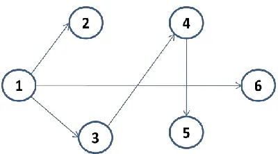
Huang et al, 2009 [4] defines a software project as a directed acyclic graph G = (V, A, S, E) where V = (1, 2, …, n) is the set of nodes representing the events (figure 1). A is the set of arcs representing the activites, (i, j)  A is the arc acyclic graph G from node i to j, and there is only one directed arc (i, j) from i to j, S V is the start node, and EV is the end node. Each activity duration time be a stochastic variable denoted  ={ij (i, j) A} .The capital cost of activity through

(i, j) is denoted Cij while the resource cost of activity through (i, j) is denoted rij.

Ruiz-Vanoye et al [23] classify the main variants of PSP:

 Resource-constrained Project Scheduling Problem (RCPSP),

 Multi-Mode Resource-Constrained Project Scheduling Problem (MRCPSP),  Construction Project Scheduling Problem (construction PSP),

 Project Scheduling Problem for Software Development (software PSP),  Payment Scheduling Problem,

 Time/cost trade-off Problem (TCTP).

Fuentes et al [24] proposed PSP with Linear Responsibility Chart (LRC) to generate an initial workload and a project initial total cost.

4

1.3 Traveling Salesman Problem

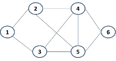
The traveling salesman problem (TSP) [10] models the situation of a travelling salesman who is required to pass through a number of cities without visiting twice the same city, so that the total travelling distances be minimal (Figure 3). According to Papadimitriou and Steiglitz [11], a Combinational Optimization Problem (COP) P = (S, f) is an optimization problem in which are given a finite set of objects S and an objective function – maximize or minimize – f :S →R+ that assigns a positive cost value to each of the objects s ∈ S. The objects are typically integer positive numbers, subsets of a set of items, permutations of a set of items, or graph structures. COP can be modelled as discrete optimization problems in which the search space is defined over a set of decision variables Xi i = 1, …, n, with discrete domains. Therefore, we will henceforth use the terms CO problem and discrete optimization problem interchangeably.

Zambito [31] describes the TSP as a graph G with a set of vertices V, a set of edges, E, and a cost, cij, associated with

each edge in E; the author mentions the solution to the TSP must return the cheapest Hamiltonian cycle of G.

Figure 3. Graph TSP representation

At [10], the author refers the TSP is a set of n towns, where the TSP can be stated as the problem of finding a minimal length tour to visit each town once. dij is the length of the path between towns i and j; in the case of Euclidean TSP, dij is the Euclidean distance between i and j. An instance of the TSP is given by a graph (N,E), where N is the set of towns

and E is the set of edges between towns. bi(t) (i=1, ..., n) is the number of ants in town i at time t and 1

( )

n

i i

m

b t







the total number of ants.

Goyal [25] Classified TSP on different instances:  Symmetric TSP

 Asymmetric TSP

The deterministic solutions to TSP are:  Linear programming [26].

 Dynamic programming formulation for an exact solution of TSP [27].  The branch and bound technique [28].

 Graphs with degree at most 3 in exponential time [29].

The non-deterministic solutions to TSP are:  Nearest neighbor algorithm [30].  Insertion algorithms [30].  K-Opt Heuristics [30].

5

There are many practical real life uses of the TSP, where each node can be presented as a city, geographical location, buildings, locations, electronic points, etc.; the most common of which are [31]:

 Transportation routing problems  Salespersons

 Music band on tour

Postal delivery person

1.4 Ant Colony Optimization (ACO)

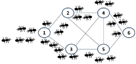
The first ACO algorithms are presented by Marco Dorigo et al at the early 1990’s [1]. The development of these algorithms was inspired by the observation of ant colonies. The behavior that provided the inspiration for ACO is the ants searching food and finding the shortest paths between the food sources and their nest. When searching for food, ants initially explore the area surrounding their nest in a random manner (Figure 2). While moving, ants leave a chemical pheromone trail on the ground. Ants can smell pheromone. When choosing their way, they tend to choose, in probability, paths marked by strong pheromone concentrations. As soon as an ant finds a food source, it evaluates the quantity and the quality of the food and carries some of it back to the nest. During the return trip, the quantity of pheromone that an ant leaves on the ground may depend on the quantity and quality of the food [11].

Figure 2. Ants path representation

Dorigo et al [21] present the General ACO meta-heuristic: procedure ACO metaheuristics

ScheduleActivities ManageAntActivity()

EvaporatePheromone() // forgetting

DaemonActions() {optional} // centralized actions local search, elitism end ScheduleActivities

end ACO metaheuristics

Steps for implementing ACO [21]:

• Choose appropriate graph representation • Define positive feedback

• Choose constructive heuristic

• Choose a model for constraint handling (tabu list at TSP)

1.4.1 Algorithms to solve TSP with ACO

6

Stutzle and Hoos [16] solved the TSP based on pheromones trail and the heuristic information between nodes choosing between the maximum and the minimum trail strenghts and constructing a valid tour according to a probability distribution proportional. They proposed a Max-Min ant System where they select the best ant to update the pheromones trail. Tsai and Tsai [18] Describes a new approach for Solving Large Traveling Salesman Problem Using Evolutionary Ant Rules for solving TSP introducing a genetic exploitation and the method nearest neighbor (NN).

Junjie and Dingwei [19] used an ACO Algorithm for multiple TSP, where the total salesmen visited every unvisited nodes selecting the next node independently.

Salami [20] proposed the ACO Genetic Algorithm (ACOG) adapting genetic operations to enhance ant movement towards solution state.

The way ant colonies function has suggested the definition of a computational paradigm, which we call Ant System This solution can apply to TSP because the solution consists on visit stages evading obstacles. Dorigo et al [11].

2. Meta-Heuristic Algorithm based on ACO, Tabu Search and PSP for TSP

A combinatorial optimization problem has a set C = {c1,…, cn} of components. A subset c1 of components represents an

optimal solution of the problem; There are a 2C _{possible solutions combination (S) and the selected solution S}

1 is feasible

if S1  S. A time function t is defined over the solution domain and the objective is to find a minimum time solution S1.

The ants move is based on stochastic local decision policy with two parameters: local pheromone update rule, which applied whilst constructing solutions and global pheromone updating rule, which applied after all ants construct a solution.

The proposed algorithm is combined well distribution strategy of initial ACO, a next-node selection with Tabu search and a PSP for assign the best way. The recognition group explores the different paths according to Tabu Search to visit every node.

The main loop consists on Estimate the effort’s cost between nodes following the pheromone trail, select the next node with the best solution f(s*), the minimal effort cost (the node with minor path, max pheromones and minor distance) and update the visited nodes.

The main target is determine the best way (optimization loop) to travel between nodes selecting the next node based on the recognition loop and the main loop.

The proposed algorithm is described as follows:

//Initialization

Set parameters, initialize pheromone trails m = nodes (cities)

costij = Travel cost between nodei and nodej

Wt = Total cost

wij = Travel Cost from nodei to nodej

distanceij = Distance between nodei and nodej

N = Total of ants

k = random number of ants N

timeij = time between nodei and nodej

antp = actual ant

// Functions

Tabu_evaluation(nodei, nodej)

7

End Tabu_evaluation

Tabu_restriction(nodeq)

For each neighbor nodeq

Tabu_evaluation (nodei, nodeq)

End For

End Tabu_restriction

Update Pheromones()

Total_Pheromonesij = Total_Pheromonesij + Pheromonesantp –

random_diffusion_pheromones End Update

max_Pheromones()

Compare k – pheromones from pathsp and select the pathp with max pheromones

End max_pheromones

min_pathp()

Compare k – pathsp and select the pathp with min total_distance

End min_path

Estimate cost_effortij(timeij, distanceij, Wt)

If (timeij > 0, distanceij > 0, Wt > 0)

cost_effortij = ((timeij* distanceij * Wt)/( timeij + distanceij + Wt))

End if End Estimate

Trace_best_way() selecting nodej to visit where (max_pheromoneij() and

min_cost_effortij() and min_pathij())

Select neighbor nodes from nodei

Compare neighbor – pathsp (pheromonesij(), cost_effortij(), pathij())

Select the best_way with (max_pheromonesij(), min_cost_effortij(),

min_pathij())

End trace_best_way

// Recognition loop

Allocate h = random number of k on initial (or random) nodei where i <= m

for each antp from k group

Select random nodej to visit

Do

Estimate timeij Estimate distanceij

Update nodes visited Update pheromones()

Assign pathp = pathp + distanceij

Tabu_restriction(nodej)

nodei= nodej

Select random nodej to visit

While nodej was not visited

end for

//Main loop n=N-k

For each ant from n group // second ants group

Allocate n = N-k ants on initial (or random) nodei where i <= n

8

Estimate cost_effortij(time, distance, Actual_weight) from neighbor nodes

Tabu_restriction(nodeq) from neighbor nodes

Select nodej to visit where ((max_pheromone() and min_pathp() and

min_cost_efforij() and minor Tabu_restriction(nodeq))

If max_pheromone() = 0

Select random nodej

End if

Update cities visited() Update pheromones() i=j

While not_visited_all_nodes()

//Optimization loop

initial (or random) nodei // the origin city

do

trace_best_way() selecting nodej to visit where (max_pheromoneij() and

min_cost_effortij() and min_pathij() and min_Tabu_restriction())

i=j

While not_visited_all_nodes()

2.1 Algorithm description

This algorithm differs from the algorithms proposed; it uses a Project Scheduling Problem (PSP) to enhance performance. It consists of three main sections: initialization, main loop and optimization loop. The main loop runs for a user defined number of iterations. These are described below:

Initialization

a. Set the initial parameters: variables, initial states, functions, inputs, outputs, initial trajectory, output trajectories. b. Initial set of nodes (cities)

c. Set initial pheromone trails value = 0. d. Set the travel costs between nodes

e. Estimate the total weight of deliver packages

f. Estimate each weight’s package to deliver on each node g. Define the total ants

h. Select an ants random number from total ants i. Set the distances between nodes

j. Each node has empty pheromones.

Functions

a. Update pheromones(): Ants leave a pheromone trail which is updated when another ant goes through the same path and randomly the trail is removing for natural conditions.

b. The max pheromones function compares the paths between the actual node with other nodes and select the path where more ants.

c. Min_path():This function aims to compare the different paths used by ants recognition group and select the minimal distance path.

d. Cost_effort: Each path between two cities laid out by the ants has a time, distance and weight carried. The effort is calculated from these factors multiplying them and dividing the result by the sum.

e. Trace_best_way():This function analyzes the different path efforts between two cities, from this analysis, we choose the path of least distance, less effort and maximum pheromone.

f. Tabu_evaluation(): This funtions estimate the effort multiplying the cost and the distance.

9

Recognition loop

a. A random ants number is allocated on initial node (or random node) to initialize the paths search (recognition group)

b. Each ant will visit every node randomly estimating the time and distance between nodes and delivering pheromones. The tabu_restriction compares the distance-cost between the actual node with neighbor nodes.

Main loop

a. Set the initial parameters with the results of initialization and recognition loop. b. Each ant is individually placed on initial state with empty memory.

c. The rest of the ants colony is allocated on the same initial node (or the same random node) from recognition group

d. Set initial pheromone trails value based on recognition group. e. Each visited city has ant’s pheromones from recognition group.

f. Construct Ant Solution while each ant has not visited every city: Each ant constructs a path by applying the transition function between node (i,j) based on the data from recognition group and the new data from actual ant; the probability of moving from node to node depend on the parameters described before.

a. Apply Local Search

b. Estimate the cost effort from actual node to neighbor nodes based on time and distance estimated by recognition group

c. Select the next node to visit based on minimize the cost effort, maximize the pheromones, minimize the path’s distance and the minor evaluation.

d. Update Trails: Evaporate a fixed proportion of the pheromone on each road. For each ant perform the “ant-cycle” pheromone update. Reinforce the best tour with a set number of “elitist ants” performing the “ant-cycle”.

e. Update the pheromones where the actual ant has passed.

f. The operations are applied to individual(s) selected from the population with a probability based on fitness. Darwinian Reproduction, Structure-Preserving Crossover or Structure-Preserving Mutation. g. End While

Optimization loop

a. Set the initial parameters with the results of initialization, recognition loop and main loop. b. Set initial pheromone trails value over initialization, recognition loop and main loop. c. Each city has a pheromones level from N group.

d. Construct the best Ant Solution: Each ant constructed a path by applying the transition function between node (i,j).

e. the best way is calculated by multiplying the distance, time and weight and divided by the sum of these parameters:

a. While not visited every city

i. max_pheromone(): Analize the paths (i,j) maximizing the pheromones level ii. min_cost_effort(): Analize the paths (i,j) minimizing the cost_effort iii. min_pathij(): select the path (i,j) minimizing the distance

iv. min_tabu_restriction(): select the node with minor evaluation. b. End While

2.2. Simulation

The 100 cities tour simulation [22] to be solved with ACO and The proposed algorithm to compare the solutions. // Initialization loop:

10

m = 100 nodes

costij = random function between 0…1

Wt = sum of random weight package delivered on nodej

distanceij = 0.0001 – 10-0000

N = Random Total ants

k = Random number of ants < N timeij = 0.001 seconds * distance * 1000

At the initial tours we presented 100 cities to visit (figure 4). Each city is represented by a node with a random distance.

Figure 4. Initial tour

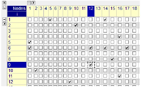
The neighbors nodes are defined randomly, allocated them with x and y coordinates. In figure 5, the node 12 has 2 neighbors: node 6 and node 9.

Figure 5. Neighborhood Allocating the cost of the nodes is done randomly between 1 and 100 (figure 6).

11

Figure 6. Aleatorial solution

The ACO Solution (Figura 7) does not present crossing ways and the results are better than AS; the time solutions increase almost 300% comparing to AS, but the solution reduced the 20% distance approximately. The effort cost is widely better if the AS effort cost is 100%, ACO presents de 85% averaged.

Figure 7. ACO solution

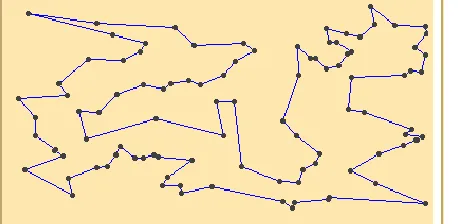
The proposed algorithm solution (Figure 8) used less memory than AS and ACO, the time solution is similar to ACO, but the effort cost is 20% averaged lowest than AS and in some cases, presents a 13% lowest from ACO.

12

2.3 Comparing solutions

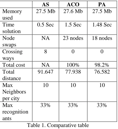
The table 1 shows the comparison between AS, ACO and the proposed algorithm (PA) results from one instance. This instance has a hundred nodes randomly distributed, ten neighbor nodes maximum, thirty-three ants from recognition group and a random weight per node.

AS ACO PA

Memory used

27.5 Mb 27.6 Mb 27.5 Mb Time

solution

0.5 Sec 1.5 Sec 1.48 Sec Node

swaps

NA 23 nodes 18 nodes Crossing

ways

8 0 0

Total cost NA 100% 98.2%

Total distance

91.647 77.938 76.582 Max

Neighbors per city

10 10 10

Max recognition ants

33% 33% 33%

Table 1. Comparative table

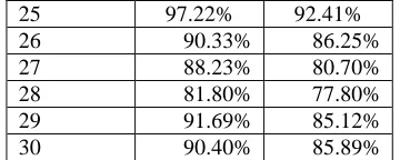
The table 2 shows the results from 30 instances where the best algorithm is SPANCO with the minimal effort cost estimation. In this table we assume the 100% effort cost is the AS traced path.

Instance ACO PA

1 85.04% 83.56%

2 98.66% 83.56%

3 97.52% 81.07%

4 97.76% 89.95%

5 88.19% 82.60%

6 92.88% 86.64%

7 94.36% 83.56%

8 93.33% 82.97%

9 90.45% 81.07%

10 93.32% 89.95%

11 87.80% 82.60%

12 89.91% 86.64%

13 94.25% 87.05%

14 88.23% 86.54%

15 91.21% 85.25%

16 88.04% 85.80%

17 93.15% 85.12%

18 86.22% 84.96%

19 87.96% 82.76%

20 91.17% 83.72%

21 83.25% 80.03%

22 92.77% 88.24%

23 85.93% 82.16%

13

25 97.22% 92.41%

26 90.33% 86.25%

27 88.23% 80.70%

28 81.80% 77.80%

29 91.69% 85.12%

30 90.40% 85.89%

Table 2. 30 effort per instance comparative table

3. Conclusions

Ruiz-Vanoye et al. [9] describes the complexity of algorithms as the way of classify the algorithms about the optimal solutions on time and efficiently and the complexity of instances as the problem complex [9]; in this way the SPANCO algorithm involves a non probabilistic steps because it based on select the best way maximizing the resources and minimizing the efforts.

The AS solution has several problems to solve TSP, the Ant colony Optimization (ACO) algorithm may produce redundant states in earlier steps, but if we combine ACO with Project Scheduling Problem (PSP) and Tabu Search adding a cost_effort function, the algorithm is better minimizing the time and effort’s costs to enhance the behavior of the inducted system.

A colony of ants moves through system states randomly based on past pheromones trails but this way not always is the best solution. If we apply PSP, the ants moves are focused on reduce the redundant states by selecting the optimum way to solve the problem.

The simulation results has a better performance selecting the best way based on pheromones trail, the minimal path, the minimal time and the minimum evaluation.

4. Related works

This is the first work introducing PSP, Tabu Search and ACO to solve TSP, in future works the researches can improve the effort_cost function or introduce new paradigms or new meta-heuristics. This solution can be applied on several problems with similar requirements.

5. Bibliography

[1] Dorigo M, Optimization, learning and natural algorithms. PhD thesis, Dipartimento di Elettronica, Politecnico di Milano, Italy, 1992 [in Italian].

[2] E. Bonabeau, M. Dorigo and G. Theraulaz, Swarm Intelligence: From Natural to Artificial Systems. New York, NY: Oxford University Press, 1999.

[3] Fuentes-Penna A., Ruiz-Vanoye J., Pathiyamattom-Joseph S. and Fernández-Medina M. A. Linear Responsibility Chart for PSP. 2011 Electronics, Robotics and Automotive Mechanics Conference

[4] Huang, W., Ling, L., Wen, B., Cao, B. (2009). Project Scheduling Problem for Software Development with Random Fuzzy Activity Duration Times. Advances in Neural Networks – ISNN 2009. 6th International Symposium on Neural Networks, ISNN 2009. Wuhan, China, May 2009 Proceedings, Part II. Springer. LNCS 5552. ISSN: 0302-9743. ISBN-10: 3-642-01509-3. ISBN.13: 978-3-642-01509-0

[5] Ruiz-Vanoye Jorge A., Pathiyamattom-Joseph Sebastian. y Fernández-Medina Miguel A. and Fuentes-Penna A. Project Scheduling Problem for Software Development Library – PSPSWDLIB. Revista de Ciências da Computação, 2010, nº5.

14

Industrial Engineering Theory, Applications and Practice, pp. 460-472, Mexico City, Mexico October 17-20, (2010) ISBN 97809652558-6-8.

[7] Jorge A. Ruiz-Vanoye, Ocotlán Díaz-Parra, Alejandro Fuentes-Penna, José C. Zavala-Díaz. Productos de Innovación Tecnológica obtenidos de imitar la Naturaleza. Revista de Educación y Divulgación Científica y Tecnológica de la UDLAP (ALEPH ZERO). Número 57, Julio - Septiembre (2010).

[8] Jorge A. Ruiz-Vanoye, Ocotlán Díaz-Parra, Felipe Cocón, Andrés Soto, Ma. De los Ángeles Buenabad Arias, Gustavo Verduzco-Reyes, Roberto Alberto-Lira. Meta-Heuristics Algorithms based on the Grouping of Animals by Social Behavior for the Traveling Salesman Problem. International Journal of Combinatorial Optimization Problems and Informatics, Vol. 3, No. 3, pp. 104-123, Sep-Dec (2012). ISSN:2007-1558.

[9] Jorge A. Ruiz-Vanoye and Ocotlán Díaz-Parra. An Overview of the Theory of Instances Computational Complexity.International. Journal of Combinatorial Optimization Problems and Informatics, Vol. 2, No. 2, May-Aug, 2010

[10] Lawler E, Lenstra JK, Rinnooy Kan AHG, Shmoys DB. The travelling Salesman problem. New York: John Wiley & Sons; 1985

[11] Marco Dorigo, Vittorio Maniezzo, and Alberto Colorni. The Ant System: Optimization by a colony of cooperating agents. IEEE Transactions on Systems, Man, and Cybernetics–Part B, Vol.26, No.1, 1996, pp.1-13

[12] Papadimitriou CH, Steiglitz K. Combinatorial optimization—Algorithms and complexity. New York: Dover; 1982. [13] S. Goss, S. Aron, J. L. Deneubourg, and J. M. Pasteels, “Self-organized shortcuts in the argentine ant,”

Naturwissenschaften, vol. 76, pp. 579–581, 1989.

[14] B. H¨olldobler and E. O. Wilson, The Ants. Berlin: Springer-Verlag, 1990.

[15] R. Beckers, J. L. Deneubourg, and S. Goss, “Trails and U-turns in the selection of the shortest path by the ant Lasius Niger,” J. Theoretical Biology, vol. 159, pp. 397–415, 1992

[16] Thomas Stutzle and Holger Hoos. MAX-MIN Ant System and Local Search for the Traveling Salesman Problem. 0-7803-3949-5/97/$10.00 0 1997 IEEE

[17] Marco Dorigo and Gianni Di Caro. Ant Colony Optimization: A New Meta-Heuristic. 0-7803-5536-9/99/$10.00 01999 IEEE

[18] Cheng-Fa Tsai and Chun- Wei Tsai. A New Approach for Solving Large Traveling Salesman Problem Using Evolutionary Ant Rules.

[19] Pan Junjie and Wang Dingwei. An Ant Colony Optimization Algorithm for Multiple Travelling Salesman Problem. Proceedings of the First International Conference on Innovative Computing, Information and Control (ICICIC'06). 0-7695-2616-0/06 $20.00 © 2006 IEEE.

[20] Nada M. A. Al Salami. Ant Colony Optimization Algorithm. UbiCC Journal, Volume 4, Number 3, August 2009 [21] Marco Dorigo and Thomas Stützle. Ant Colony Optimization Book. The MIT Press. Editorial Springer.

[22] Optimization Software for Mathematical Programming. http://www.aimms.com. Last visited: 02/02/2013.

[23] Jorge A. Ruiz-Vanoye, Ocotlán Díaz-Parra, José C. Zavala-Díaz, Alejandro Fuentes-Penna, Juan C. Olivares-Rojas. Models, resources and activities of project scheduling problems. International Journal of Industrial Engineering-Theory Applications and Practice. ISSN: 1943-670X

[24]Fuentes-Penna A., Ruiz-Vanoye J.A., Pathiyamattom-Joseph S. and Fernández-Medina M.A. 2011 Electronics, Robotics and Automotive Mechanics Conference 978-0-7695-4563-9/11 $26.00 © 2011 IEEE. DOI 10.1109/CERMA.2011.80 461.

[25] Sanchit Goyal. A Survey on Travelling Salesman Problem.

[26] Dantzig GB, Fulkerson DR, Johnson SM (1954). Solution of a Large-scale Traveling Salesman Problem.” Operations Research, 2, 393410.

[27] Held M, Karp RM (1962). A Dynamic Programming Approach to Sequencing Problems”. Journal of SIAM, 10, 196 - 210.

[28] Little JDC, Murty KG, Sweeney WD, Karel C, ”An Algorithm for the Traveling Salesman Problem,” Operational Research, vol. 11, no. 6, pp. 972-989, 1963.

[29] Eppstein, D. 2003b. The traveling salesman problem for cubic graphs. In Proceedings of the 8th Workshop on Algorithms and Data Structures. Lecture Notes in Computer Science, vol. 2748. Springer-Verlag, New York, 307– 318.

[30] Hahsler, Michael; Hornik, Kurt (2007), ”TSP Infrastructure for the Traveling Salesperson Problem

15

[32] Hertz A. and de Werra D. L. Using Tabu Search Techniques for Graph Coloring. Computing by Springer-Verlag. 1987. Computing 39, pp 345- 351.

[33] Glover F. Future paths for integer programming and links to artificial intelligence, Comp. Oper. Res. 13 (1986)533-549.