Asymptotically optimal path planning with integrated local optimisation for robotic vine pruning

(1)

Asymptotically optimal path

planning with integrated local

optimisation for robotic vine

pruning

Scott Paulin

A thesis presented for the degree of Doctor of Philosophy

in

Mechanical Engineering at the

University of Canterbury, Christchurch, New Zealand.

(2)

(3)

ABSTRACT

Grapes are an important crop to New Zealand and the rest of the world. Vineyards cover 75,000km2 worldwide and New Zealand wine exports were valued at $1.57 billion in 2016. Grape vines are pruned annually to improve yield. Pruning is done manually for many vine species and is the most labour intensive and expensive task for the vineyard.

A robotic pruning system is being developed at the University of Canterbury to automate cane pruning, where canes are selectively removed to leave a small number of long healthy canes. The robot uses stereo-cameras to construct a 3D model of the vines and an AI system to determine where vines should be pruned. A UR5 robot arm with a spinning router is then used to make the cuts. An online path planning algorithm is required to plan collision free paths for the robot arm to reach cut-points. The path planner should quickly compute paths that are fast to execute after being converted to trajectories so that the robot can operate efficiently. This thesis proposes new path planning approaches for quickly computing paths that are fast to execute when converted to trajectories.

(4)

robot relies on its path planner being able to quickly find paths that can be converted to fast-to-execute trajectories.

Collision detection speed is often the bottleneck in performance for many sampling based path planners. Fast path planning can be achieved by using an efficient collision detector. This research proposes a new collision detection algorithm that exploits the structure of grape vines to provide fast collision detection. This collision detector takes 3.0×10−6 seconds on average to classify the collision status of a robot configuration and is 50 times faster than the popular Flexible Collision Library [Pan et al 2012]. This speed-up in collision detection results in a 27 times reduction in path planning times.

Two approaches to finding fast-to-execute paths are to use an asymptotically op-timal path planner, or to use a local optimiser. Asymptotically opop-timal planners are guaranteed to eventually find the optimal, e.g. shortest, solution but can be slow. Local optimisers are capable of quickly improving a solution with respect to a cost function such as path length, but are not guaranteed to find the optimal solution. The approach proposed in this thesis integrates an asymptotically optimal planner with a local optimiser to speed up the search for short paths while retaining the planner’s asymptotic optimality. The asymptotically optimal RRTConnect* planner integrated with a ‘short cut’ local optimiser found paths that were 31% faster to execute than those found by RRTConnect* without the local optimiser for the vine pruning robot given three seconds of planning time.

(5)

v

robot.

(6)

(7)

LIST OF FIGURES

1.1 Vine pruning robot [Botterill et al 2016]. 2

1.2 3D reconstruction of grape vines [Botterill et al 2016]. 3

1.3 Robot arm making a cut [Botterill et al 2016]. 3

1.4 How the path planning module typically fits in with the rest of a robotic

system. 4

1.5 Planning node from Fig. 1.4. Tref is a reference trajectory and c0, ..., cn

denotes a sequence of robot configurations. 5

1.6 Two poses for the UR5 robot arm that put the end-effector at the same

position. 5

2.1 Roadmap with two connected components and a brown obstacle. 12

2.2 An example of a multiple query planner searching for a path from qstart

toqgoalthrough its roadmap G. 12

2.3 GrowRoadmap procedure for the PRM path planner. 12

2.4 Tree of motions rooted at the blue circle with a brown obstacle. 13

2.5 An example of a single query planner finding a path from qstart toqgoal. 14

2.6 Expansion process for RRT. 15

2.7 Locally optimal insertion of a new vertex into an incremental planner’s

(12)

2.8 Focussed sampling after an initial solution has been found. 19

2.9 Path plan and corresponding tree of motions for a bidirectional search

between the start (S) and goal (G) vertices. 20

2.10 Lazy path plan between the start (S) and goal (G) vertices with an

invalid motion. 21

2.11 RRT with an abstracted goal representation. 26

2.12 Weed spraying robot environment. 31

2.13 Proposed apple harvesting robot path planning scene [Nguyen et al 2014]. 31

3.1 UR5 robot arm with labelled joints and dimensions in mm. 36

3.2 Individual joint positions for collision-free configurations from one

mil-lion randomly sampled configurations. 38

3.3 Mounting the UR5 on a flat surface (brown) causes its configuration space to be disjoint depending on the position of the shoulder lift joint. 39

3.4 Annotated image of vine pruning robot setup in ROS’s RVIZ

visualisa-tion software. 41

3.5 Vine pruning robot hub (a) and inside the hub (b) [Botterill et al 2016]. 43

3.6 Labelled robot arm [Botterill et al 2016]. 43

3.7 Cutting tool dimensions. 44

3.8 Robot arm reaching to make the last of six cuts on a plant. 44

3.9 Robot arm at the start and end of a cut swipe motion 44

3.10 Separation cut [Botterill et al 2016]. 45

3.11 Reference frames for the cameras and planning software. 46

3.12 Information flow for vine pruning robot. 48

(13)

LIST OF FIGURES xiii

3.14 UR5 robot simulator. 49

3.15 Path planning to cut a vine through with a router. 51

3.16 Procedure to attempt to calculate a swipe motion to make a cut. 51

3.17 Distance from optimal cut point for solved cuts obtained in simulation from data captured on a row of Sauvignon Blanc at Lincoln University. 52

3.18 Two reconstructed grape vines with modified cut motions shown in green. 53

3.19 Cubicle picking scenario. 53

3.20 Dimensions for cubicles experiment setup. 55

3.21 Gripper for cubicles experiment with dimensions. 56

3.22 Information flow for the simulated cubicles picking robot. 56

4.1 Discrete motion validation with at most L distance between collision

checked points. 58

4.2 Cross-sectional view of a capsule approximated by a sphere and ray. 62

4.3 Adaptive safety margin applied to a vine. 63

4.4 One dimensional sweep and prune. 64

4.5 Full collision checking of an object with the rest of the scene. 64

4.6 Full collision checking of the robot arm with itself and the environment. 65

4.7 The safety margin applied to an obstacle. 66

4.8 Breakdown of computation time for specialised collision detector. 67

4.9 Computation and execution times when using FCL or the proposed

spe-cialised collision detector. 68

5.1 Path plan and corresponding tree of motions for a bidirectional search. 72

(14)

5.3 Expansion process for RRT. 74

5.4 Path planner success rates for vine pruning experiment. 78

5.5 Path planner computation times for vine pruning. 79

5.6 Lengths of paths found by each planner for vine pruning. 79

5.7 Execution time for paths found by each planner. 81

6.1 RRT* insertion of the yellow vertex. 87

6.2 Multiple restarts of RRTConnect with short-cutting. 89

6.3 RRTConnect* with short-cutting. 91

6.4 Insertion of a path p into a planner’s graph G using RRT*’s insertion procedure for the objective of minimising Euclidean path length. 93

6.5 Means for 304 successful grape vine planning queries. 95

6.6 Means for 144 cubicles queries. 96

7.1 Two poses for the UR5 robot arm that put the end-effector at the same

position illustrating workspace redundancy. 100

7.2 The blue dots show equivalent configurations shown in blue for a robot arm with two joints that can each operate in the range [−2π,2π). 104

7.3 Algorithm for computing goal configurations for a robot using its workspace

and configuration space redundancy. 105

7.4 Path length and execution times using different numbers of random goals and the improvement over using one goal for the vine pruning experiment.108

7.5 Ranking of goal configuration used in shortest path over time for vine

(15)

LIST OF FIGURES xv

7.6 Path length and execution times using different numbers of the closest goal configurations and the improvement over using one goal for the vine

pruning experiment. 110

7.7 Ranking of goal configuration used in shortest path over time for vine

pruning experiment. 111

7.8 Path length and execution times using different numbers of random goals and the improvement over using one goal for the cubicles experiment. 112

7.9 Ranking of goal configuration used in shortest path over time for cubicles

experiment. 113

7.10 Path length and execution times using different numbers of closest goal configurations and the improvement over using one goal for the cubicles

experiment. 114

7.11 Ranking of goal configuration used in shortest path over time for cubicles

(16)

(17)

LIST OF TABLES

2.1 Asymptotically optimal variations of feasible path planners. 15

2.2 Comparison of agricultural robots that use joint space path planning. 32

4.1 Configurations of specialised collision detector and FCL 62

4.2 Mean times for full collision checking with smart safety margin 65

4.3 Mean times for self collision checking with smart safety margin 65

4.4 How the specialised collision detector identifies that pairs of objects are not intersecting when the input robot state is not in collision. 66

5.1 Path planners tested 76

5.2 Parameters used for each planner in experiments 77

6.1 Summary of planners evaluated 91

6.2 Parameters used in vine pruning robot tests 92

6.3 Parameters used in cubicle picking tests 92

7.1 Goal types and descriptions 102

1 Neighbourhood definitions for some popular asymptotically optimal

(18)

(19)

ACKNOWLEDGEMENTS

I would like to thank my supervisors Professor XiaoQi Chen, Associate Professor Richard Green and Dr. Tom Botterill for the advice and feedback they have provided me with during my studies. In particular, I would like to thank Tom for his advice, critical feedback, technical discussions and patience, which have all greatly contributed to my PhD experience and the skills that I take forward.

(20)

(21)

Chapter 1 INTRODUCTION

Grapes are an important crop to New Zealand and the rest of the world. Vineyards cover 75,000km2 worldwide [FAO 2017] and New Zealand wine exports were valued at $1.57 billion in 2016 [NZ Winegrowers 2016]. Grape vines are pruned annually during the winter to improve yield and prevent disease [Kilby 1999]. Many vines in New Zealand arecane pruned, where branches are selectively cut to leave two or three long healthy canes [Christensen 2000]. Pruning is done manually for many vine species and is the most labour intensive and expensive task for the vineyard [Dryden 2014]. It is also one of the few tasks on the vineyard that has not been mechanised.

(22)

the-sis proposes new path planning approaches that are tested on this vine pruning robot. The robot is fully described in Chapter 3.

A number of other robots have been developed to perform labour intensive agricul-tural tasks such as kiwi-fruit harvesting [Scarfe et al 2009], apple harvesting [Nguyen et al 2013, Davidson et al 2016], precision weeding [Lee et al 2014], and melon har-vesting [Edan 1995, Edan et al 2000] among others [Hayashi et al 2010, Chatzimichali et al 2009, Liu et al 2012, Cai Jianrong, Wang Feng, L¨uQiang 2009, Noguchi and Terao 1997]. Like the vine pruning robot, all of these robots perform their tasks (harvesting or weeding) while stationary, with the exception of the melon harvesting robot [Edan et al 2000].

In their review of 50 recent agricultural robots, Bac et al [2014] found that sensing the environment and robot cycle times were two important challenges. The robot’s cycle time is directly affected by the computation time and quality, e.g. shortness, of collision free paths found by the path planner. Imperfect sensing results in the path planner having a model of the world with errors. If these errors are not accounted for, the robot may collide with obstacles while following a path that the planner has computed to be collision free.

(23)

3

(a) Grape vines to be reconstructed.

[image:23.595.113.525.511.748.2]

(b) Reconstructed grape vines. Optimal cuts are marked in blue and vines to be removed are shown in orange.

Figure 1.2: 3D reconstruction of grape vines [Botterill et al 2016].

(24)

1.1 ROBOT ARM PATH PLANNING

Path planners use sensor data to compute a path for the robot to achieve its task without colliding with the environment or itself. This path is then parameterised by the relative time that the robot will reach each waypoint, forming a trajectory. The trajectory is then executed by the robot, and the environment may be altered if objects are moved (Fig. 1.4).

To speed up computation time, path planners run on robots without differential constraints, e.g. many robot arms, ignore the robot’s velocity and accelerations. These velocities and accelerations are computed to minimise the execution time of the path after the planner has terminated with a valid path (Fig. 1.5). Quick-to-execute paths can still be found by the planner because execution time is often strongly correlated with the path’s Euclidean length (see the figures in Chapt. 6), even though other factors such as the accelerations of the robot’s joints influence the execution time of the path.

Robot arms are typically required to perform tasks in their workspace, e.g. reach the fruit at a certain Cartesian position. The workspace of a robot arm is typically two or three dimensional and consists of all the points reachable by the robot. Alternatively, the robot’s position can be represented by its joint angles, or configuration. A robot’s configuration space describes all sets of joint angles that can be obtained by the robot.

Planning Robot controller

Environment Sensing

Control logic Tref

Actuation

W

orld

mo

del

Task spec.

(25)

1.1 ROBOT ARM PATH PLANNING 5

Path planner c0, ..., cn Time stamping Tref

W

orld

mo

del

Task spec.

Figure 1.5: Planning node from Fig. 1.4. Tref is a reference trajectory and c0, ..., cn

denotes a sequence of robot configurations.

Forward and Inverse kinematics are used to map the robot’s pose in its workspace to its configuration. Forward kinematics maps a configuration to link poses in the workspace. This can often be solved analytically for serial manipulators. Inverse kine-matics maps the pose of one or more links to configuration space. Solutions can be found using numerical optimisation algorithms such as Levenberg–Marquardt [Mar-quardt and Donald. W. 1963]. Analytical solutions exist for some robot arms e.g. the UR5 [Hawkins 2013]. One end-effector pose for the robot can sometimes be achieved by the robot in more than one configuration (Fig. 7.1).

(26)

1.2 MOTIVATION

Enabling robots to perform their tasks quickly is an important problem for many different robot systems. Bac et al [2014] use cycle time as a performance indicator in their review of 50 recent robotic systems for harvesting fruit, and cite it as an important economic factor for agricultural robots.

The primary motivation of this thesis is to develop new approaches for path plan-ning that allow the vine pruplan-ning robot to quickly prune vines. To achieve this, my approaches should quickly compute high quality (e.g. short) paths for the robot arm. The new approaches developed in this thesis can be used on different robots. Some of these approaches are tested on a secondary robot task as well as being tested on the vine pruning robot.

1.3 THESIS ORGANISATION

Chapter 2 contains a review of the path planning literature relevant to agricultural robots that use a robot arm. This covers approaches that have been used to speed up and/or improve the quality of paths found for robot arms. It also covers approaches for dealing with ‘real world’ effects such as sensor uncertainty.

Chapter 3 describes the experiment setup. This details about the input data, how the robot arm was controlled, how cut positions were selected and how cuts were performed. A secondary experiment, a robot for reaching into cubicles, is also described. This secondary robot was used for testing the proposed approaches in Chapters 6 and 7 to verify that they were applicable to robotic tasks other than grape vine pruning.

(27)

1.3 THESIS ORGANISATION 7

In Chapter 5 the performance of 17 commonly used sampling based path planners is compared. The most successful planners for this task are identified, and one of them is selected to be further improved in subsequent chapters.

Chapter 6 presents a path planning algorithm that integrates an asymptotically optimal path planner with a local optimiser to speed up the search for high quality paths. By integrating a short-cutting local optimiser the planner was able to find paths that had a 31% shorter execution time when converted to trajectories after three seconds of computation time.

Many robot arms can achieve their tasks using more than one goal configuration, in this thesis these arms are called redundant. Chapter 7 shows how these extra goal configurations can be used by an asymptotically optimal path planner to quickly find high quality paths. By using these extra goal configurations, paths that had a 58% lower execution after being converted to trajectories could be found.

(28)

(29)

Chapter 2 PATH PLANNING LITERATURE REVIEW

Path planners often operate in the robot’s configuration space [Lozano perez 1983] to find collision free paths. A configuration represents the position of each of the robot’s joints, this is six dimensional for the six degree of freedom UR5 robot arm used for vine pruning. The configuration space,C, can be split into Cfree and Cobs. Cfree is the

set of all configurations where the robot is not in collision with the environment or itself. Cobs is the set of configurations where the robot is in collision with itself or the

environment. Computing an explicit representation of configuration space for many robot arms is prohibitively expensive.

Sampling-based planners [Kavraki et al 1996, LaValle 1998, Sucan and Kavraki 2010, Sucan et al 2012] are by far the most widely used methods used for online planning for robot arms and other high degree of freedom robots because they do not require an explicit representation of the robot’s configuration space. They use a collision de-tector to classify sampled configurations as either in Cfree or Cobs. Artificial

Poten-tial Fields [Khatib 1986, Newman and Hogan 1987, Hwang et al 1992, Barraquand et al 1992] and geometry-based methods [Lozano prez and Wesley 1979, Schwartz and Sharir 1983] have also been developed, but are limited to simple environments [Koren and Borenstein 1991] because they get stuck in local minima or require an explicit representation of the robot’s configuration space.

(30)

planners attempt to quickly find a solution and terminate as soon as one is found. Feasible planners can return poor, e.g. long, solutions because they do not optimize solutions. Optimizing planners attempt to find high-quality, e.g. short, solutions within a set computation time or number of iterations.

Many sampling based path planners are probabilistically complete [LaValle 1998, Kuffner and Lavalle 2000, Sucan and Kavraki 2009a]. As the number of samples drawn by the planner approaches infinity the probability that a solution is found, given a robustly feasible solution [Karaman and Frazzoli 2011] exists, approaches 1.

Some sampling-based path planners are also asymptotically optimal. The cost of the best path found by an asymptotically optimal planner will approach the cost of the optimal path, given a robustly optimal path [Karaman and Frazzoli 2011] exists, as the number of iterations approaches infinity.

Sampling-based path planners often use an acyclic graph data-structure referred to as a tree. Vertices in the graph represent sampled configurations and edges represent local paths between these configurations. These local paths can be straight lines in configuration space, e.g. when planning for a robot arm, or curved arcs when plan-ning for car robots. The planner returns a path, which is a sequence of vertices and edges connecting the start and goal configurations. Graph vertices are fast to collision check because they represent a single point in configuration space, while edges can be expensive to check because they represent a path.

(31)

Fraz-11

zoli 2011] or Sparse Roadmap Spanners (SPARS) [Dobson and Bekris 2014].

Multiple-query planners, e.g. Probabilistic Roadmap (PRM) [Kavraki et al 1996], often construct a graph with many edges between vertices as shown in Fig. 2.1, this is often referred to as a roadmap. It should be noted that straight lines in configuration space do not represent straight line motions in the workspace, for a robot arm these often result in arcing motions. The roadmap is expanded during planning as shown in Fig. 2.2. The routineGrowRoadmap expands the roadmap, andShortestPath returns the shortest path through the roadmap between two vertices e.g. by using A* graph search [Hart and Nils 1968]. Multiple query planners are effective when they are used for more than one query in an environment because they can re-use the roadmap. Roadmaps can be slow to construct because they often have a large number of edges that need to be collision checked. This means multiple-query planners can be slow if they are only required for few planning queries.

The PRM is the most well known multiple-query sampling based path planner. To solve a planning query the PRM grows its roadmap until the start and goal configu-ration are within one connected component as shown in Fig. 2.2. The PRM roadmap is typically grown by batch-sampling and then connecting these new samples into the roadmap as shown in Fig. 2.3. The BatchSampleVertices method returns a number of collision-free vertices, where the exact number might be a parameter set by the user. The original implementation used a batch size of one. TheConnectNewSamples routine forms collision-free edges between the newly sampled vertices and the existing roadmap. Some variations of PRM, e.g. k-PRM1, attempt to connect each new ver-tex to the nearest k vertices. Other variations, e.g. r-PRM, attempt to connect new vertices to other vertices within a radius. The original PRM implementation only at-tempted to connect vertices if they were in different connected components. When the start and goal vertices are in the same connected component a graph search algorithm, e.g. A*, is used to recover the path between the start and goal vertices.

Single query planners are effective at quickly finding collision free paths. These

(32)

Figure 2.1: Roadmap with two connected components and a brown obstacle. Filled circles show vertices, arrows show edge directions. The query start vertex is shown in blue and goal vertex is shown in red.

1: function Query(G= (V, E), qstart, qgoal)

2: do

3: G ←GrowRoadmap(G)

4: whileqstart andqgoal are not in the same connected component

5: return ShortestPath(G, qstart, qgoal)

6: end function

Figure 2.2: An example of a multiple query planner searching for a path from qstart to

qgoalthrough its roadmap G.

1: function GrowRoadmap(G= (V, E))

2: Vsampled ← BatchSampleVertices()

3: G← ConnectNewSamples(G, Vsampled)

4: return G

5: end function

(33)

13

planners build a directed tree as shown in Fig. 2.4. The vertices of this tree represent points in the robot’s configuration space and edges in this tree represent paths between these vertices. This tree has few edges because each vertex is only connected to one other vertex. Having few edges makes trees relatively quick to construct because fewer expensive edge collision checks need to be performed. However, having few edges means that trees are not usually useful for planning queries other than the one they were constructed for. Fig. 2.5 shows a procedure for solving a planning query with a single query planner. The function GrowTree expands the planner’s tree. Trace constructs the path between the start and goal vertex by recursively following each parent’s vertex starting with the goal.

Figure 2.4: Tree of motions rooted at the blue circle with a brown obstacle. Filled circles show vertices, arrows show edge directions. The goal vertex is shown in red.

(34)

1: function Query(qstart, qgoal)

2: Initialise Gto be a graph with a single vertexvstart atqstart

3: vgoal← qgoal

4: do

5: G ←GrowTree(G, vgoal)

6: whilevgoal∈/ G

7: return Trace(G, vgoal)

8: end function

Figure 2.5: An example of a single query planner finding a path from qstart to qgoal.

GrowTree may take additional parameters.

to the new vertex is collision free then an edge to the new vertex is formed and it is added to the tree.

Planning from experience approaches combine the fast plan times of single-query planners with the ability to reuse computation. A single-query planner is used to quickly compute collision-free paths for planning queries, and these paths are stored in a graph [Phillips et al 2012, Coleman et al 2015] or a path database [Berenson et al 2012]. Eventually some planning queries can quickly be satisfied by using data from the graph or database, without needing to invoke the single-query planner.

2.1 ASYMPTOTICALLY OPTIMAL MOTION PLANNING

Asymptotically optimal planners eventually converge to the optimal solution [Kara-man and Frazzoli 2011]. They are similar to probabilistically complete feasible path planners, but the edges of all vertices must remain optimal within a local neighbour-hood, see Appendix 8.2. A number of feasible path planners have been adapted to be

asymptotically optimal (Tab. 2.1).

(35)

neigh-2.1 ASYMPTOTICALLY OPTIMAL MOTION PLANNING 15

(a) Tree of motions. (b) New vertex is sampled (green).

r

(c) Vertex is saturated. (d) Vertex is added to tree.

Figure 2.6: Expansion process for RRT with ranger. The start vertex is shown in blue, the goal vertex is shown in red. The green vertex is sampled, saturated, and added to the tree.

Table 2.1: Asymptotically optimal variations of feasible path planners.

Feasible planner Optimal variation

RRT RRT* [Karaman and Frazzoli 2011]

RRTConnect RRTConnect* [Akgun and Stilman 2011, Klemm

et al 2015, Jordan and Perez 2013]

PRM PRM* [Karaman and Frazzoli 2011]

(36)

bouring vertex that minimises the cost to arrive at the new vertex. The edges from the remaining vertices in the neighbourhood must then be updated if the new vertex provides a better path to arrive as shown in Fig. 2.7. When a new vertex, vnew is

sampled its neighbourhood is calculated as either all vertices within a radius or the nearest k vertices (Fig. 2.7a). An edge is then formed between vnew and the vertex

in the planner’s tree that minimises the cost to arrive at vnew (Fig. 2.7b). Edges to

other vertices within the neighbourhood may also be updated (Fig. 2.7c). Updating or forming edges is expensive because it requires collision checking.

Some optimizing planners are asymptotically optimal [Karaman and Frazzoli 2011] and will eventually converge to the optimal solution [Gammell et al 2015, Janson et al 2015, Karaman and Frazzoli 2011]. Other optimizing planners are asymptotically near-optimal and will eventually converge to a near-optimal solution [Arslan 2013, Dob-son and Bekris 2014, Otte and Frazzoli 2015, Salzman and Halperin 2016].

2.1.1 Batch sampling

Optimal sampling-based path planners can be split into those that perform incremental search, and those that perform batch sampling. RRT* [Karaman and Frazzoli 2011] and other incremental sampling based path planners attempt to add one vertex to their tree of motions at each iteration. This makes them well suited to finding fine motion plans in large configuration spaces.

s

(a) New vertex is sampled and its neighbourhood is calculated.

s

(b) New vertex is added to the planner’s tree.

s

(c) Neighbouring vertices are updated.

(37)

2.1 ASYMPTOTICALLY OPTIMAL MOTION PLANNING 17

Batch sampling based single query motion planners, e.g. Fast Marching Trees (FMT*) [Janson et al 2015] and Batch Informed Trees (BIT*) [Gammell et al 2015], compute a batch of collision-free samples and then attempt to find high quality collision free paths through these samples. Unlike incremental planners, batch planners do not modify samples to bring them closer to the planners graph (or tree). The tree is then constructed in a lazy fashion, where vertices are added in order from most promising to least promising. Vertices that cannot be used to find a lower cost, e.g. shorter, path through the graph than the current best path are not added, saving computation time. These planners can have faster convergence times than incremental planners in some problems [Gammell et al 2015, Janson et al 2015, Starek et al 2015] because they use this information about how promising a state is to guide the search.

Batch sampling planners are not suited to finding fine motion plans in large con-figuration spaces. This is because the granularity of the plan that they can find is governed by how densely the configuration space is sampled. Dense sampling of large configuration spaces can require a large number of samples to be generated and colli-sion checked. This large number of samples can also take a long time to process. BIT* partially remedies this by drawing multiple smaller batches of samples from subsets of configuration space that decrease in size. This biasing is well suited to problems where an initial solution can be quickly found and the optimal solution is a close to the straight line from the start to the goal. Having a smaller batch size limits the planner’s ability to only add promising states into it’s search graph. In this thesis incremental sampling-based path planners are used because the vine pruning robot requires fine motion plans to get the cutting tool close to cut points that are very close to obstacles (other parts of the plant). A plan resolution of approximately 1cm in the workspace may be required for areas near cuts.

2.1.2 Focussed search heuristic

(38)

it spends more time processing samples that cannot possibly be used to improve on the best solution [Gammell et al 2014]. This can be remedied by focussing the planner’s search to useful regions of configuration space [Gammell et al 2014] and rejecting new samples that cannot be used to improve on the planner’s best solution [Akgun and Stilman 2011] without sacrificing the optimality properties of the planner.

The region of the robot’s configuration space where samples can be used to improve the best path can be defined as:

Xf ={x∈X|f(x)< cbest}, (2.1)

wherexis a configuration in the robots configuration spaceX, this is a six dimensional point for the UR5. cbest is the cost of the best path found so far by the planner. f(x)

is the optimal cost of a collision free path that goes from the start configuration to the goal throughx. In practice,f(x) can be approximated by the admissible cost ofx. The admissible cost never overestimates f(x) and is specific to the optimization objective being used2. An informed sampler [Gammell et al 2014] can be used to draw samples directly from Xf once an initial solution has been found.

The focussed search procedure is outlined in Fig. 2.8. The informed sampler sam-ples vertices from within Xf which is shown as an ellipse. Even though the newly

sampled green vertex is within Xf it cannot possibly be used to find a shorter path

than the dark blue one that has already been found. The green vertex is rejected according to the heuristic in Akgun and Stilman [2011].

2.2 BIDIRECTIONAL SEARCH

Some path planners use a bidirectional search to find collision free paths faster [Kuffner and Lavalle 2000, Sucan and Kavraki 2010, Hsu et al 1999, S´anchez and Latombe 2003a], and/or speed up convergence [Akgun and Stilman 2011, Jordan and Perez 2013, Klemm et al 2015, Starek et al 2015]. Two trees are grown toward each other, one from the start

(39)

2.2 BIDIRECTIONAL SEARCH 19

Figure 2.8: Focussed sampling after an initial solution (dark blue) has been found. The brown rectangle represents an obstacle. The dashed ellipse shows the regionXf.

state and one from the goal state. Paths are found when the two trees are connected (Fig. 2.9). Bidirectional search works well when the goal configuration is difficult to reach, e.g. is in a cluttered part of configuration space. This is because the goal tree is a bigger target for the start tree than a single configuration.

(40)

S G 1 2 3 4 5 6 7 8 9 10

(a) Path plan from a bidirectional search. Connecting motion is shown in light gray.

S

1 3 2

4 5 6 7 8 G 10 9

(b) Start (S) and goal (G) trees of motions with the connecting motion in light gray.

Figure 2.9: Path plan and corresponding tree of motions for a bidirectional search between the start (S) and goal (G) vertices.

2.3 LAZY COLLISION CHECKING

A large amount of path planning time is spent collision checking edges that will not be part of the final solution. Some single query and multiple query planners attempt to speed up planning by delaying the collision checking of edges until a path is found between the start and the goal (but vertices are still checked) [Bohlin and Kavraki 2000, Bohlin and Kavraki 2001, Gasparri et al 2009, S´anchez and Latombe 2003a], these planners are referred to as ‘lazy’. Once a path is found, the edges are collision checked. If they are all collision free the planner can terminate with a solution, otherwise edges that are in collision are pruned from the planer’s graph. Lazy single query planners will additionally prune all descendants of invalid edges to prevent adding disconnected components (Fig. 2.10).

A number of lazy planners have been developed for feasible, e.g. Lazy-PRM [Bohlin and Kavraki 2000] and SBL3 [S´anchez and Latombe 2003a], and asymptotically (near) optimal planning, e.g. Lazy-PRM* [Hauser 2015] and Lazy-LBTRRT [Salzman and Halperin 2016]. Choudhury et al [2016a] extend the Lazy-PRM* to evaluate paths that are less likely to be in collision first to speed up the search for initial solutions.

(41)

2.4 SAMPLE BIASING 21 S G 1 2 3 4 5 6 7 8

(a) Lazy path plan with an invalid path be-tween milestones one and four.

S

1 2

3 4 5

6 7

8

G

(b) Tree of motions corresponding to lazy path plan. Motions and milestones in light gray are to be removed due to the invalid mo-tion between milestones one and four.

Figure 2.10: Lazy path plan between the start (S) and goal (G) vertices with an invalid motion.

Planners with lazy collision evaluation perform well when there is a small chance of edges being in collision. This mostly depends on the configuration space being planned in and the length of edges in the planner’s graph, which can often be controlled with a range parameter. If too many edges are in collision the planner will often have to discard many edges and restart planning with a smaller graph. If few edges are in collision then a lazy planner is more likely to find a collision-free solution earlier than a non-lazy planner because it performs less collision detection.

2.4 SAMPLE BIASING

Sample biasing is a common approach for improving computation time of feasible path planners and the convergence time of optimizing planners. Goal biasing is the most common form of sample biasing. Many incremental single-query planners will sample a goal state with a constant probability to encourage growth toward the goal [LaValle 1998, Otte and Frazzoli 2015, Hsu et al 1999, LaValle 2001, Ladd and Kavraki 2005].

(42)

et al 1998] are used to generate samples near obstacles. The bridge test for nar-row passages [Hsu et al 2003] and medial axis sampling to maximise obstacle clear-ance [Wilmarth et al 1999]. There is some contention about the effectiveness of these approaches, with Geraerts [2006] finding that they only work well for specific problems and can significantly degrade the planner’s performance in other problems.

Thomas et al [2007] also identify that certain sampling schemes are only effective in certain problems. They propose a framework for combining multiple sampling schemes, where each sampler biases the sample returned by the previous sampler. Although this approach allows the strengths of different samplers to be combined, the planner’s performance is now dependant on the combination of samplers that is used. Picking a good combination of samplers for a particular problem may be difficult in practice.

Zhong and Liu [2016] propose a hybrid sampling scheme that combines a uniform, a Gaussian, and a bridge test sampler. The configuration space is split into regions by a classifier. Samples for each region are drawn independently from the three samplers in different proportions as dictated by the classifier. Ideally the individual samplers get used in local regions that pose problems which they were designed for e.g. the bridge sampler gets used in regions with narrow passages. Regions where it is difficult to sample collision-free configurations are additionally sampled more heavily than those where collision-free configurations can be sampled.

Both Thomas et al [2007] and Geraerts [2006] agree that connecting samples, rather than generating samples in difficult to sample regions of configuration space, is a more important problem in motion planning for batch sampling planners. Incremental plan-ners, e.g. RRT, are better at joining samples because they relocate new samples to be a maximum of range from the planner’s graph. However, this also means that sample biasing is difficult to achieve with incremental planners because the samples may be moved by the planner.

(43)

2.5 PLANNING WITH UNCERTAINTY 23

variation of RRT*. Nasir et al [2013] implement a more exploitive variation of the approach by Alterovitz et al [2011] with their RRT*-Smart planner. RRT*-Smart biases sampling toward only the best path found so far. RRT*-Smart is particularly effective compared to RRT* when there are few, e.g. 1-3, homotopy classes in the problem as shown in the results in Nasir et al [2013]. Alterovitz et al [2011] perform few experiments with their biased RRT* planner, but it should outperform RRT*-Smart on problems with a large number of homotopy classes because it is less greedy.

2.5 PLANNING WITH UNCERTAINTY

In real robots, the environment generated through sensor data is not the same as the real world model. This results in path plans being computed that appear collision-free, but in fact result in collisions when used on a real robot. To overcome this, path plan-ners can incorporate information about the certainty of obstacle locations [Chakravorty and Kumar 2011, Bopardikar et al 2016, Valencia et al 2010]. Errors can sometimes be modelled by Gaussians [Missiuro and Roy 2006] when this information is not known. Sometimes Gaussians are also a poor model, e.g. for errors resulting in incorrect cor-respondences in the 3D reconstruction.

When errors are difficult to model, one can use an optimizing planner such as RRT* to maximise obstacle clearance. This could be computationally expensive due to the slow convergence of RRT* and the extra collision detection time required to compute distances to nearest obstacles.

Another approach is to introduce a safety margin by increasing the obstacle size [Fahimi 2009]. This enforces a minimum clearance in computed plans from the model of the

(44)

2.6 USING OBSTACLE PROXIMITY TO REDUCE COLLISION

CHECKING

Some approaches to path planning store obstacle proximity information and use it to speed up, or avoid, future collision checks. This information is often stored as a volume in the robot’s configuration space or workspace that is known to be collision free. Approaches that store configuration space approaches, e.g. configuration space safety certificates [Bialkowski et al 2016], can only be used when the configuration space distance between a configuration and the nearest obstacle can be computed, e.g. when an explicit representation of the obstacles in configuration space is known. This is very difficult when an explicit representation of obstacles is not known e.g. for robot arm path planning.

In many cases, e.g. planning for a robot arm, this is very difficult.

Collision free volumes in the workspace can be computed by enlarging the robot model [Vahrenkamp and Asfour 2007, Bialkowski et al 2016] or fitting other volumes. A common approach is to fit bubbles around robot poses in the workspace. Early approaches compute very conservative bubbles that only extend to the nearest obsta-cle [Quinlan and Khatib 1993, Bertram et al 2006, Lacevic and Rocco 2010]. These bub-bles could be very small in cluttered environments when the distance to the nearest ob-stacle is small in at least one direction. Later approaches find less conservative volumes by performing dilations [Bialkowski et al 2016] or finding free workspace ‘slices’ [Ade-movic and Lacevic 2016]. Finding large collision free volumes is advantageous because it may mean that more collision checks can be bypassed. Workspace collision-free volumes can then be used for guiding the planner’s search as well as bypassing some collision checking [Lacevic and Rocco 2013, Ademovic and Lacevic 2014, Lacevic et al 2016].

2.7 PATH OPTIMISATION

(45)

2.8 PATH PLANNING WITH REDUNDANT MANIPULATORS 25

solution. This initial solution influences the quality of the optimised path because these algorithms only optimize locally. Short-cutting [Berchtold and Glavina 1994, Geraerts et al 2007, Hauser and Ng thow hing 2010] for reducing path length and sequential convex optimization approaches [Kalakrishnan et al 2011, Schulman et al 2014, Zucker et al 2013] have been shown to work well on robot arms.

A common approach to finding short paths is to find an initial collision-free solution with a feasible planner, e.g. RRTConnect [Kuffner and Lavalle 2000], and to optimise this path with a local optimiser e.g. short-cutting. Another approach is to perform multiple restarts of the feasible planner, optimise each solution and return the best solution. This has been shown to work well in empirical experiments when compared to asymptotically optimal planners [Luo and Hauser 2014].

After short-cutting, paths will tend to come very close to obstacles. This is fine in simulation, but poses problems when used with a real robot that has error in the environment model. On the vine pruning robot there are errors in the 3D reconstruction which means paths that appear valid to the planner result in collisions between the robot arm and obstacles. One method to mitigate this is by adding a safety margin to the obstacles, modelling them as larger than they are [Fahimi 2009]. This approach is not suitable for vine pruning out-of-the box because the targets for the cutting tool are obstacles for the rest of the robot. This could mean that with added thickness to obstacles the targets cannot be reached without collision.

Path smoothing is performed after planning and short-cutting. This prevents jerky robot motions. A common implementation is to use interpolation and short-cutting on subdivided paths [Sucan et al 2012].

2.8 PATH PLANNING WITH REDUNDANT MANIPULATORS

(46)

1: function RRT(start, goal, range, goal bias)

2: G← start

3: do

4: rand ←A random number in [0,1)

5: if rand < goal bias then

6: vsampled ← A configuration sampled fromgoal

7: else

8: vsampled ← A random configuration

9: end if

10: vnear ← The closest vertex inG tovsampled

11: // Setvsampled to be at most range fromvnear.

12: vsampled ← Interpolate(vnear, vsampled, range)

13: if The path from vnear tovsampled is collision-free then

14: e← The edge fromvnear tovsampled

15: G← G∪e, vsampled

16: end if

17: whileG does not contain a vertex that satisfiesgoal

18: vgoal← The vertex in Gthat satisfies goal.

19: return Trace(G, vgoal)

[image:46.595.70.483.111.397.2]

20: end function

Figure 2.11: RRT with an abstracted goal representation.

Some approaches for path planning with redundant robot arms rely on using a goal representation other than a single configuration. The representation of a goal for a sam-pling based path planner, such as RRT, can be abstracted as shown in Fig. 2.11. The goal variable may represent a single configuration, multiple configurations or anything else that can have configurations sampled from it.

In many cases the goal is represented by one configuration [Lee et al 2014, Coleman et al 2015, Stilman et al 2007, Hirano et al 2005] that satisfies the robot’s task. This means that the path planner is constrained to finding a collision free path that ends at one particular configuration, when there may be many, possibly better, goal config-urations that satisfy the robot’s task requirements. The single goal configuration can be sampled using an inverse kinematic solver, e.g. TRAC-IK [Beeson and Ames 2015], that finds solutions that optimise an objective e.g. manipulability or distance from obstacles.

(47)

configu-2.8 PATH PLANNING WITH REDUNDANT MANIPULATORS 27

rations. Each goal configuration represents one way that the robot can achieve its task. This approach has been used with feasible path planners to improve their suc-cess rates [Drumwright and Ng thow hing 2006, Dalibard et al 2009, Ellekilde and Petersen 2013]. This approach requires a fixed number of goal configurations to be computed before planning starts. Using a large number of goal configurations enables the planner to exploit the robot arm’s redundancy, however, these configurations may take significant time to compute. Additional goal configurations may be useful for difficult planning queries, but might not be required for simple queries.

Instead of representing a constant number of configurations, goal could represent a workspace goal region [Berenson and Ferguson 2009, Berenson et al 2011]. The goal maintains a list of configurations, but has is capable of sampling more goal configura-tions that satisfy the robot’s task. During some iteraconfigura-tions a constant number of goal configurations are sampled and added togoal’slist of target configurations. This means that the number of goal configurations grows as the planner takes more computation time to find a solution. Less time is spent computing inverse kinematic solutions in queries where the planner can quickly find a solution.

Bertram et al [2006] propose a variation of the RRT algorithm that does not require configuration space goals to be computed before planning, it plans toward workspace goals. Their planner constructs a tree, similar to how RRT constructs a tree but without goal biasing. The vertices added to the tree are ranked according to how close they put the robot to a workspace goal and the distance to the nearest obstacle. On some iterations, the planner selects the highest ranked vertex in the tree and attempts to extend it in a random direction. This new extension is only kept if it results in the tree becoming closer to the workspace goal. Extensions then continue in the same direction in configuration space until an extension fails. Vertices are removed from the ranked list when extensions from them have failed a specific number of times.

(48)

highest ranking in a random direction, it is extended directly toward the workspace goal using the robot’s Jacobian.

Keselman et al [2014] use two instances of the JT-RRT planner in their Forage-RRT planner. Forage-Forage-RRT constructs a course tree with one of the JT-Forage-RRT planners. The purpose of this tree is to achieve large configuration space coverage. Each vertex in this tree is added to a queue. Vertices in this queue are sorted such that the highest rank vertex is closest to a workspace goal. The second JT-RRT planner is then used to perform a fine grained search, expanding from the highest ranked vertices. The purpose of this fine-grained JT-RRT is to extend vertices from the coarse grained JT-RRT’s tree into the goal. Expansions that fail to extend into the goal result in the vertex being removed from the queue of promising vertices.

Dragan et al [2011a] modified the Covariant Hamiltonian Optimization for Motion Planning (CHOMP) [Zucker et al 2013] trajectory optimizer to be able to handle a set of goal configurations. They found that considering a set of goals improved the paths that were found by CHOMP. An extension to this work considered using a Support Vector Machine (SVM) [Boser et al 1992] to pick a good goal configuration to use with CHOMP before planning [Dragan et al 2011b]. These results suggest that specifying a goal as a set of configurations may allow asymptotically optimal planners, e.g. RRTConnect* [Akgun and Stilman 2011, Klemm et al 2015, Jordan and Perez 2013], to find better paths.

2.9 PATH PLANNING IN OTHER AGRICULTURAL ROBOTS

(49)

2.9 PATH PLANNING IN OTHER AGRICULTURAL ROBOTS 29

The vine pruning robot being developed at the Israel Institute of Technology relies on a human to specify cut points. Cuts are made using secateurs that are attached to the end of a six degree of freedom robot arm. A camera is used to provide feedback on the relative position of the secateurs to the cut position while individual joints on the robot arm are rotated to bring the secateurs closer to the cut position. Collision detection is not performed.

Two previous agricultural robots, one for apple harvesting [Nguyen et al 2013] and one for precision weeding [Lee et al 2014], compute collision free paths using joint space planning for high degree of freedom robot arms. The weed spraying robot uses the same six degree of freedom UR5 robot arm as the vine pruner. Before the robot is used, a database of paths is computed for the robot arm using the RRTConnect planner. This data-base is constructed assuming that there will only ever be one obstacle in the environment and that it can be encapsulated with a single fixed-size sphere directly below the robot arm (Fig. 2.12). At runtime, a path is selected from the database and it’s start and end configurations are repaired to match that of the planning query. CHOMP is then used to optimise the path. This approach is not appropriate for the vine pruning robot because it relies on the environment always being the same and cannot account for the variability of vines.

The proposed apple harvesting robot uses a custom built nine degree of freedom manipulator for picking. They tested a number of feasible sampling-based path planners and found that RRTConnect had the smallest computation times. Sensing errors are not accounted for and may cause collisions when the real robot is used.

Both the proposed apple harvester (Fig. 2.13) and weed spraying robots (Fig. 2.12) only consider one robot arm configuration to reach each target, when there are actually many. Considering multiple goal configurations would likely improve plan execution times of the trajectories that result from the plans found by the planner.

(50)

position of these is not known prior to operation. Implementing the system used by the apple harvester could be a good start for developing a system that path plans for vine pruning.

(51)

2.9 PATH PLANNING IN OTHER AGRICULTURAL ROBOTS 31

Figure 2.12: Weed spraying robot environment. Weeds (targets) lie on the ground plane and the plant (obstacle) is approximated by a single sphere [Lee et al 2014].

(52)

Table 2.2: Comparison of agricultural robots that use joint space path planning.

Robot Apple

har-vester

Weed sprayer Vine pruner

Robot arm 9 dof custom built 6 dof UR5 6 dof UR5

Environment obstacles

Apple tree with-out leaves (figure 2.13)

Plant approxi-mated by a sphere (figure 2.12)

Grape vines,

wires, and posts.

Queries Pick apples

at-tached to the tree

Spray weeds ran-domly located on ground

Cut specific vines

Obstacle positions known before operation

No Yes No

Account for sensing un-certainty

Yes by fitting large sphere over obstacle

No Required

2.10 SUMMARY

Recent research into robot arms has focussed on using sampling-based motion planning. This is because sampling-based methods do not require an explicit representation of configuration space and can compute collision-free paths reasonably quickly in more than two dimensions.

Collision detection is one of the main computation time bottle-necks for sampling-based path planners. Previous research has attempted to reduce the number of collision checks using heuristics e.g. by using workspace obstacle proximity and/or lazy collision checking. In Chapter 4 I propose a fast collision detector that exploits the structure of grape vines to speed up path planning.

(53)

2.10 SUMMARY 33

vine pruning robot’s reliability without preventing it from getting close to canes for pruning.

Quickly finding high-quality paths is an important problem in path planning as it allows robots to operate efficiently. Asymptotically optimal path planners, e.g. RRT*, can find the optimal solution, but are slow to converge. Local optimisers, e.g. short-cutting, can quickly improve an initial solution, but do not converge to the optimal solution. In Chapter 6 an approach is proposed that integrates a short-cutting local optimiser with the asymptotically optimal RRTConnect* path planner to quickly find short paths.

(54)

(55)

Chapter 3 DEVELOPMENT OF A PROTOTYPE ROBOTIC

PRUNING SYSTEM

The approaches proposed in this thesis were evaluated on a vine pruning robot. The approaches described in Chapters 6 and 7 were additionally evaluated on a robot for reaching into cubicles to see how they would perform on a task other than vine pruning. Both experiments make use of the six degree of freedom Universal Robot (UR) UR5 robot arm.

3.1 UR5 ROBOT ARM

The UR5 robot arm has six rotational joints that are capable of making two full rota-tions. The robot arm with its joints labelled is shown in Fig. 3.1 and its specifications can be found in Appendix. 8.2. I used the open source Universal Robot drivers1. Some of the joints of the UR5 robot arm had to be limited to account for un-avoidable colli-sions between the robot arm and itself, or the robot arm and the wall it was mounted on.

3.1.1 Limiting joints

The elbow joint of the UR5 robot arm used in our experiments was limited to the range [−π, π). This is because the arm has a self collision when the elbow joint is close to

±π as shown in Fig. 3.2. This self collision causes the UR5’s configuration space to

(56)

(57)

3.1 UR5 ROBOT ARM 37

be split into three disjoint sets depending on whether the elbow joint is in [−2π,−π), [π, π) or [π,2π). Since these sets are disjoint, it is not possible to find a collision-free path where the start and goal positions of the elbow joint are in different sets. This has been breaking the path planning with the UR5 for some time and had been thought to be a software bug. I have reported this issue to the Universal Robot repository on GitHub.

(58)

(a) UR5 in self collision. The self collision is circled in blue.

0 1000

2000

3000

4000

5000

6000

7000

8000

9000

Base

Shoulder

0 1000

2000

3000

4000

5000

6000

7000

8000

9000

Elbow

Wrist 1

−6 −4 −2 0

2

4

6

0 1000

2000

3000

4000

5000

6000

7000

8000

9000

Wrist 2

−6 −4 −2 0

2

4

6 Wrist 3

Nu

mb

er

of

va

lid

co

nfi

gu

rat

ion

s

Nu

mb

er

of

va

lid

co

nfi

gu

rat

ion

s

Joint position [rad]

Nu

mb

er

of

va

lid

co

nfi

gu

rat

ion

s

Joint position [rad]

Collision free configurations for UR5

(59)

3.1 UR5 ROBOT ARM 39

(a) UR5 in collision with mounting wall.

0 1000

2000

3000

4000

5000

6000

7000

8000

9000

Base

Shoulder

0 1000

2000

3000

4000

5000

6000

7000

8000

9000

Elbow

Wrist 1

−6 −4 −2 0

2

4

6

0 1000

2000

3000

4000

5000

6000

7000

8000

9000

Wrist 2

−6 −4 −2 0

2

4

6 Wrist 3

Nu

mb

er

of

va

lid

co

nfi

gu

rat

ion

s

Nu

mb

er

of

va

lid

co

nfi

gu

rat

ion

s

Joint position [rad]

Nu

mb

er

of

va

lid

co

nfi

gu

rat

ion

s

Joint position [rad]

Collision free configurations for UR5 with backwall

(60)

3.2 ROBOT OPERATING SYSTEM AND MOVEIT SETUP

The Robot Operating System (ROS) [Quigley et al 2009] and Moveit [Chitta et al 2012] middleware libraries were used for both the vine pruning and cubicle picking robots. ROS and Moveit use a distributed architecture. At runtime various parts of the software are executed asynchronously in different nodes. Nodes are stand-alone executables. They may communicate with each other at runtime by publishing or subscribing to topics.

(61)

3.3 VINE PRUNING ROBOT 41

Figure 3.4: Annotated image of vine pruning robot setup in ROS’s RVIZ visualisation software.

3.3 VINE PRUNING ROBOT

The vine pruning robot straddles over the row of grape vines it is pruning (Fig. 3.5). This hub blocks out sunlight so that lighting can be controlled using LEDs. While the robot is being pushed along the row of vines, it uses stereo cameras to capture images of the vines. These images are used by a 3D reconstruction algorithm [Botterill et al 2013] to build a model of the plants.

(62)

the cuts.

The robot arm (Fig. 3.6) has a mill-end cutting bit mounted that is used to cut the vines (Fig. 3.7). The mill end is powered with a 100 W 24,000 revolution-per-minute Maxon brushless DC motor.

The hub is stopped when the next plant to prune is located in front of the robot arm. The cut positions are then modified to positions where the robot arm can make cuts without colliding with itself or the rest of the plant (Sec. 3.3.2). A collision free path for the robot arm to reach each cut is computed using the path planner, and executed on the UR5 robot arm (Fig. 3.8). When the arm reaches each cut-point it swipes through it with the router (Fig. 3.9). If this is successful the vine will be cut (Fig. 3.10).

(63)

(a) Hub for the vine pruning robot. (b) Inside the vine pruning robot hub.

Figure 3.5: Vine pruning robot hub (a) and inside the hub (b) [Botterill et al 2016].

(64)

Figure 3.7: Cutting tool dimensions.

Figure 3.8: Robot arm reaching to make the last of six cuts on a plant. The vine on the right has had an adaptive safety margin applied [Botterill et al 2016].

[image:64.595.183.368.113.330.2]

(a) Robot arm at start of swipe motion. (b) Robot arm at end of swipe motion.

(65)

[image:65.595.153.483.110.375.2]

Figure 3.10: Separation cut [Botterill et al 2016].

3.3.1 Software architecture

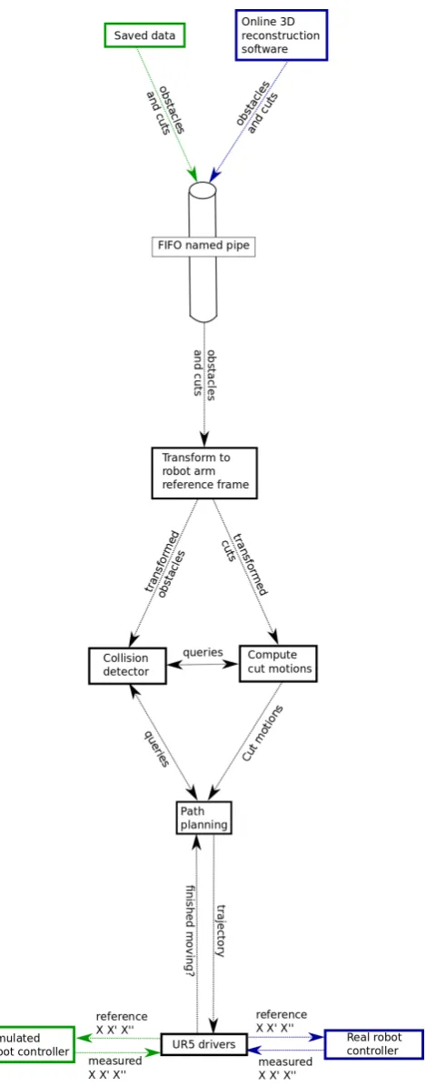
The path planning software was designed to run on data streamed from either the online 3D reconstruction algorithm, or saved data as shown in Fig. 3.12. The paths taken by the software when the reconstruction software was being run (e.g. during a field test) are shown in blue. The paths taken by the software when saved 3D reconstruction data was being used are shown in green.

The 3D reconstruction software streamed a model of the environment (see Ap-pendix 8.2 for some sample data for one plant). The canes and trunk were represented as 3D polylines (lines that pass through a series of way points) and the plant’s head was represented with spheres (Fig. 3.13). The cutpoints found by the AI algorithm were represented by the Global Unique IDentifier (GUID) of the cane they were on and a distance from the start of the cane. Knowing what cane a cut was on was important for computing swipe motions. All of this data was represented in a reference frame located at the start of the row.

(66)

[image:66.595.173.379.110.346.2]

Figure 3.11: Reference frames for the cameras and planning software. The reference frame used by the Universal Robot controller is located in the same position as the one used by the planning software but rotated 90 degrees counter clockwise.

used by the path planning from the camera reference frame that is used by the 3D reconstruction software as shown in Fig. 3.11. The 4x4 transformation matrix from the camera frame to the planning frame was calculated with the use of a marker attached to the end of the robot arm. The 3D reconstruction software was used to compute the pose of the marker relative to the camera frame, and the robot arm’s forward kinematics routine was used to compute the pose of the marker relative to the planning reference frame. Knowing the pose of the marker relative to both of these reference frames the transform from the camera frame to the planning frame was computed.

Points output from the 3D reconstruction software were transformed into the path planning reference frame as follows:

Xplanning=Tcamera to planningXcamera (3.1)

(67)

refer-3.3 VINE PRUNING ROBOT 47

ence frame to the path planning reference frame.

The path planning module was isolated from the input data source (online 3D reconstruction software or saved data) by a First In First Out (FIFO) named pipe. When the 3D reconstruction software was running the vines and cutpoints were passed on to the named pipe. If saved data was being used it was read directly from file as if a named pipe was being used. This meant that the path planning module had the same interfaces regardless of whether the robot was being used in the field or being tested in simulation.

(68)

[image:68.595.165.400.116.714.2]

(69)

[image:69.595.147.494.132.361.2]

(a) Raw image of a vine. (b) Annotated image of a vine.

Figure 3.13: Example of a raw vine image before 3D reconstruction has been per-formed (a) and this image annotated with the cane, trunk and head features found by the reconstruction software labelled (b).

[image:69.595.156.484.468.728.2]

(70)

3.3.2 Computing cut motions

To make a cut the robot arm had to swipe a spinning mill end through the vine. The swipe motion had to start 4cm before the cane and end 6cm after as shown in Fig. 3.15. The 4cm before the vine was to account for some reconstruction error in the model of the vine. The 6cm after the cut position was to make sure a separation cut was performed, using shorter distances often resulted in the cane bending out of the way of the router without a cut being performed. To ensure that the mill could separate the cane at the cutpoint the direction of the swiping motion, the cane and the mill end all had to be perpendicular to each other.

The best places to make each cut were computed using AI algorithm [Corbett davies et al 2012]. This algorithm did not account for collisions between the robot arm and itself, or collisions between the robot arm and the environment. This meant that it was not always possible to cut the vines at positions specified by this algorithm using the UR5 robot arm.

The procedure for computing a swipe motion is outlined in Fig. 3.16. A tool direc-tion perpendicular to the cane’s direcdirec-tion is sampled with a bias to direcdirec-tions away from the robot’s base. A swipe direction perpendicular to both the cane and tool directions is then calculated. The SampleSwipeConfigs function then calculates configurations for the start middle and end points of the swipe motion using an inverse kinematic solver. The middle configuration is calculated first and then the start and end configurations are computed considering the swipe direction and its length (Fig. 3.15). If the path found by interpolating between start, middle and end is collision free (ignoring colli-sions between the cutting tool and cane to be cut) it is returned, otherwise failure is returned.

(71)

4cm 6cm

[image:71.595.237.401.151.347.2]

Cut motion

Figure 3.15: Path planning to cut a vine through with a router. The dashed lines represent unconstrained path plans. The solid line shows the 10cm swipe motion that is computed before any path planning is performed.

1: function ComputeSwipeMotion(cane dir, position)

2: tool dir ←Randomly sampled tool direction perpendicular to cane dir 3: swipe dir ←Direction perpendicular to cane dir

4: start, middle, end ← SampleSwipeConfigs(position, cane dir, tool dir, swipe dir)

5: swipe motion←Path made by interpolating between start, middle and end

6: // Ignore collisions between cutting tool and cane being cut

7: if swipe motion is collision freethen

8: return swipe motion

9: else

10: return Failure

11: end if

12: end function

[image:71.595.110.524.490.695.2]

(72)

[image:72.595.100.448.289.546.2]

the cane ensures that the algorithm does not always fail to find swipe motions when none are possible using the initial cut position. The algorithm was limited to 5000 iterations in the interest of limiting computation time. The cut positions were moved by 0.06mm after each unsuccessful iteration to ensure that cuts were never made more than 30cm from their ideal position. On average 82% of cuts could have swipe motions found for them. Fig. 3.17 shows how far the cut position had to be moved from the position supplied by the AI algorithm to get a collision free cut motion.

Asymptotically optimal path planning with integrated local optimisation for robotic vine pruning