Research Paper
A Fast-Multipole Unified Technique for the Analysis of Potential Problems
with the Boundary Element Methods
NEY AUGUSTO DUMONT* and HÉLVIO DE FARIAS COSTA PEIXOTO
Civil Engineering Department, Pontifical Catholic University of Rio de Janeiro, Brazil
(Received on 05 May 2016; Accepted on 12 May 2016)
The proposed developments are based on a consistent implementation of the conventional, collocation boundary element method (BEM). A scheme is used to expand a generic (not problem-dependent) fundamental solution about hierarchical levels of source and field poles, which is particularly advantageous to make the technique seamlessly applicable to 2D and 3D problems of elasticity or potential, in terms of different types of curved elements for generally complicated geometry and topology. The proposed compact algorithm is more straightforward to lay out and seems to be more efficient than the
ones available in the technical literature – particularly because the outermost loop refers to field nodes and geometry, in
what may be called a reverse implementation. Some numerical results are shown for the conventional BEM, with validation and assessment for a few simple, but very large-scale, 2D potential problems with complicated geometry and topology for constant, linear and quadratic elements. Since iterative solvers are not required in this first step of numerical simulations, an isolated assessment of accuracy, computational effort and storage allocation of the proposed fast multipole technique becomes possible.
Keywords: Boundary Elements, Fast Multipole Methods, Variational Methods
*Author for Correspondence: E-mail: [email protected], [email protected] Proc Indian Natn Sci Acad 82 No. 2 June Spl Issue 2016 pp. 289-299
Printed in India. DOI: 10.16943/ptinsa/2016/48420
Introduction
The fast multipole technique (Greengard and Rokhlin, 1987), combined with an iterative solver such as the GMRES, can speed up the complete solution time of a problem with N unknowns from order O(N)2 to O(N
log N) – or evenO(N), as suggested by (Liu, 2009) and corroborated in the present developments – while
requiring computer storage that is only a small fraction of what would be allocated for a different numerical method.
The present research work is part of the studies carried out by the second author (Peixoto, 2014) together with Novelino (2015) to develop a robust and efficient fast multipole code applicable to problems with generally curved boundaries, in a framework that is almost completely independent from the underlying fundamental solution (Peixoto et. al., 2015, 2015a). The basic concept of the fast multipole method (FMM), with the expansion of the fundamental solution about successive layers of source and field poles, is described in a compact algorithm that is more
straightforward to lay out and promises to be more efficient than the ones available in the technical literature (Nishimura, 2002; Liu and Nishimura, 2006; Liu, 2009).
This paper proposes a scheme for expansions of a generic fundamental solution about hierarchical levels of source and field poles, which makes the fast-multipole technique directly applicable to different kinds of potential and elasticity problems. The proposed hierarchical tree of poles is built upon a topological concept of superelements inside superelements, which in part circumvents the need of evaluating geometrical distances between nodes as well as the need of concepts such as quadtrees or octrees for 2D or 3D problems, as basically adopted since the inception of the FMM (Liu, 2009).
Proposed FM Algorithm for a General, Complex Function
·
z– z0 = difference between the source point z0 and the field point z.· zc= point about which the fundamental solution will be expanded for the field point z.
· zL= point about which the fundamental solution will be expanded for the source point z0.
Expansions about successively farther poleszck, k = 1, 2, …,nc (where, by definition, zc0 zc) and
l
L
z , l = 1, 2, …,nL (where, by definition, zL0 zL) are also undertaken.
A generic fundamental solution for 2D problems is expanded as
1 0 1 1 0 1 1
1
(
)
(
)
(
1)!
1
(
)
(
)
(
1)!
nknl nk nl
n
i c
i
n
j L i j c L
j
f z
z
P z
z
i
P z
z Q
z
z
j
(1)for truncation order given by max
1 1
0 0 0
(
nk) /(
)
, (
nl) /(
)
n n
c L
z
z
z
z
z
z
z
z
and with P(z) and Q(z) defined as
2 3 1
( ) 1 n
P z z z z z (2)
1 1 ( ) ( ) ( ) ( ) n n
f z f z
Q z f z
z z
(3)
In general, the higher derivatives of the fundamental solution tend rapidly to zero when evaluated for large arguments.
Equation (1) is the starting point for a procedure that leads to a computationally fast and economical
evaluation of a given fundamental solution
f z
(
z
0)
for a very large number of source points z0 and of field points z by means of a sufficiently approximateexpression. As shown,
f z
(
z
0)
is expanded in terms of successive arrays of source poles zLl aswell as field poles zck. The expansion ends up with a
series of products of binomials i( nk)
c
P zz and
0 ( nl)
i L
P z z , which are independent from the complexity of the function
f z
(
z
0)
, multiplied by functions Q zi( Lnl zcnk) that are given as( Lnl cnk)
f z z and its 2n first derivatives, for the expansion indicated in Eq. (1). Although these latter functions may be computationally intensive to evaluate, they are only needed for the multiplication
of the arrays of poles represented by zLl and zck.
Then, the evaluation of Q zi( Lnl zcnk) may end up
orders of magnitude less intensive than the direct
evaluation of
f z
(
z
0)
for all source and field points.Expansion of P zi( zck) and P zj( Lnl z0) About
Successive Poles
In Eq. (1), the superscripts nk and nl are the highest levels of field and source poles used in a given
expansion. The binomials P zi( zcl) defined in Eq.
(2) are expressed for a lower-level pole zcl1 exactly as
1 1
, 1 1
1
(
l)
(
l)
(
l l)
i
i c j i j j c i j c c
j
P z z
C
P z z
P
z
z
(4)where Cij = 1 if i = 1 or j = 1 , otherwise,Cij = Ci–1,j+
Ci,j–1. In Eq. (4), Pi 1 j(zcl1 zcl) is defined as in
Eq. (2) since the argument refers to two consecutive
levels. On the other hand, P zj( zcl1) is recursively evaluated according to Eq. (4) until the lowest level
0
j c
P z
z
is obtained. With this recursive approach, the binomials P zi( zcnk) and P zj( Lnl z0) alwaysend up expressed in terms of arguments given as differences of poles in two consecutive levels.
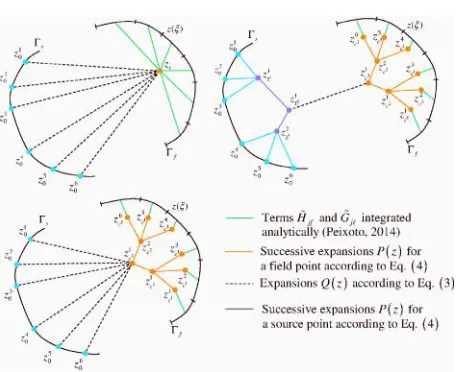
pole zc (upper left), about three successive layers of poles zc (lower left) and, moreover, source points expanded about two layers of poles zL (upper right). The continuous lines starting from the boundary f stand for analytical integrations of the BEM matrices for fast-multipole matrix-vector products
corresponding to
H
jf andG
j in Eqs. (11) and (12),as proposed in Peixoto (2014).
Hierarchical Refinement Algorithm
Figure 2 shows the schemes of three different elements considered in the present algorithm, as taken out of a general 2D mesh corresponding to a given level of refinement (Dumont, 2012). The splitting algorithm for constant elements is the same one for linear elements. A corresponding algorithm has also been implemented for 3D problems (Dumont and Aguilar, 2011). The element numbering of the reference level leads immediately to the numbering of the splitted elements, as each element is splitted into two. The created nodes (indicated by dashed circles in Fig. 2) are sequentially numbered as they appear in the splitting process, so that their global numbering does not become sequential along the boundary. The element numbering leads to the straightforward identification of adjacent split elements at each refinement level.
Figure 3 shows three cases of possible refinements, with nc = 2, 4 or 8 children elements after an element splitting.
Implemented FM Algorithm
This section describes a compact version of the implemented fast-multipole algorithm. The number of code lines is actually very small. However, as the algorithm calls a recursive routine (PoleExpansion) inside another recursive routine (Adjacencies), this makes it fairly convoluted and difficult to explain verbally, although the flowcharts can be easily translated into a code. The basic version presented
below gives an overview of the algorithm’s four major
routines: Main, Adjacencies, Source and PoleExpansion.
The procedure Main (Fig. 4) loads the input data, generates the hierarchical mesh according to the
Fig. 1: Schematic representations of expansions about field and source poles (according to Peixoto et al., 2015a)
Fig. 2: Scheme of three different elements that are split each into two sub-elements (Dumont, 2012)
[image:3.612.67.295.76.262.2] [image:3.612.357.512.77.242.2] [image:3.612.317.547.309.471.2]concepts briefly discussed in the Introduction and evaluates the kernel expansions according to Eq. (3). Then it executes a small loop over all elements of the first level (k = 0) of the hierarchical mesh in order to create the adjacency structure for each macro-element (ie), carrying out, at the same time, all the possible field evaluations for the child elements of element ie.
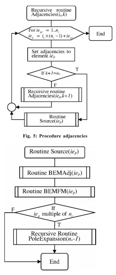
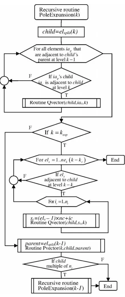
The routine Adjacencies (Fig. 5) assembles the adjacency structure, and when it reaches the most refined level (k = nv), it calls the routine Source. This routine (Fig. 6) handles integrations in terms of the conventional BEM matrix-vector products (routine BEMAdj) for the adjacent elements, as well as in terms of FM expansions (routine BEMFM). The analytical integrations carried out in the frame of the routine BEMFM refer to the closest field pole and are successively stored for use with far-field elements in the routine PoleExpansion. The routine Source also leads to the successive expansion of the FM integration
terms, thus delivering data information to the upper refinement levels, if this is the case, by calling the routine PoleExpansion.
Finally, the recursive routine PoleExpansion (Fig. 7) delivers the FM-integrated data to the source poles that are considered sufficiently far by calling the routine Qvector to evaluate the Q vectors presented in Eq. and then evaluating the expansion series for the source point, Eq. (3). It also checks if the level k = kexphas been reached, as expansions stop at this level, indicating that the results obtained so far are
Fig. 4: Procedure main
Fig. 5: Procedure adjacencies
[image:4.612.335.539.74.556.2] [image:4.612.108.263.83.412.2] [image:4.612.343.505.321.555.2]directly delivered to the remaining source points. If k = kexp has not been reached, the routine calls routine Pvector to convey the obtained data to the upper pole levels and, when all the elements of level k have been processed, calls itself (thus recursively) to proceed to the immediately upper refinement level of the hierarchical structure.
Boundary Element Implementation
For a potential problem, the double-layer potential matrix H and the single-layer potential matrix G of the conventional boundary element method are given for the continuity equation
Hd = Gt (5)
(body source not considered, for simplicity) of the nodal potentials d and the boundary nodal flux attributes in terms of the boundary integrals (Brebbia
et al., 1984)
* 0
* 0
( ) ( ) ( ) ( ),
( ) ( ) ( ),
sf ks k f
s s
H q z z z z d z
G z z q z d z
(6)
where
q
*js(
z
z
0)
and *0
( )
s z z
are the flux and
potential fundamental solutions of the potential problem
– which have global support – and (z) is the integration boundary. The subscript s refers to a given source node (at which the unit point source of the singular fundamental solution is applied) and the subscripts f (which stands for field) and (also a field reference) indicate the nodes to which the
potential-interpolation functionf( ( ))z and the flux-interpolation function
q z
( ( ))
are referred. In the above equation and in the following, repeated indicesmean summation.
k( )
z
are the Cartesian components of the outward unity vector to(z), and( )
f z
formally comes from the piecewise (with local support) interpolation of potentials (z) along the
boundary: ( )z f( )z df, where df are the nodal potentials. In a usual isoparametric representation, potential and geometry are represented identically for each one of their Cartesian components, so that
( ) ( ( ))
f z f z
are actually replaced with shape
functions
N
k( )
, for a given boundary segment, with(0,1)
or
( 1,1)
, depending on the preferred parametric representation. Forz
z
0, strong andweak singularities must be taken care of in the evaluation of H and G. However, this issue can be
[image:5.612.75.294.77.595.2]disregarded in the present developments, which are actually only concerned with what occurs when z and
z0 are very far from each other. The Jacobian used in
the definition ofj( )z cancels out with the Jacobian of d ( ) z = J z( ) d, in terms of the parametric variable. Then, expanding
q
*js(
z
z
0)
according toEq. (1) ends up with the evaluation of a polynomial integral corresponding to the first of Eq. (6). For the single-layer potential matrix G, it is proposed that the
usual interpolation polynomials
q
of normal fluxes in Eq. (6) be replaced with(at )
/
,
q
q
J
J
(7)where
J
(at ) is the value of the Jacobian at the point characterized by the subscript (Dumont, 2010; Dumont and Aguilar, 2012). Nothing changes formally in the developments of the BEM, except that the numerical integration of the matrix G becomes much easier and actually more consistent as compared to proposed implementations given in the technicalliterature (Dumont, 2010). In fact, J cancels out in the product
q
d
in Eq. (6) forq
defined as suggested, and the integrand of G, in the frame of a fast multipole implementation, also becomes a polynomial, independently from the assumed kernel*
s
. In a practical implementation, the functions
( ( ))
q z
are replaced with the same shape functions( )
k
N
used to represent potential, although the context differs conceptually, as G, among other features, is in general a rectangular matrix ( in general spans a larger number of nodes than f).As proposed, let
z
N
k( )
z
k be the complex geometric representation of a boundary segment, for a 2D implementation, expressed in terms of the nodalpoints zkand the shape functions
N
k( )
, which are also used to interpolate potential as well as normal fluxes, as described above. Then, the only integrations that need to be carried out for a given boundary segmentseg in the evaluation of the matrices of Eq.(6) in the framework of the fast multipole developments represented by Eq. (1) are for terms of H and G defined similarly to Eq. (1) as
1
0
( )d
( )
( )
( )d
seg
jf j c
j k k c
f
l l i
H
P z
z z N
P N
z
z N
z N
(8)
1 0( )
( )
d
( )d
segj j c
j k k c
G
P z
z N
P N
z
z N
(9)where, recalling, repeated indices mean summation,
in this case covering all shape functions
N
k( )
of a boundary segment representation, and a prime ( )means derivative with respect to. Since the Jacobian inherent to d in the above integrals cancels out, the
indicated interval
(0,1)
is actually irrelevant. Inthe first row of the above equation, the term
N
l
( )
z
lcomes from the complex representation of
k( )
z
along the boundary segment. The subscript j refers to one of the terms in the adopted expansion of Eq. (4), whereas i refers to each of the boundary element nodes. In the present implementation for 2D problems (Novelino, 2015), either linear, quadratic or cubic boundary elements may be represented. Constant elements are considered in a separate implementation. The main feature of the proposed implementation of
the FMM is that the arrays
H
jf andG
j given abovebecome ultimately expressed as polynomials of the differences of the nodal coordinates of the boundary segment to the immediate pole,
, with
1
1,
i
z
iz
ci
o
e
(10)where oe = 1, 2, 3 for linear, quadratic or cubic boundary elements. As an illustration for quadratic elements (3 nodes),
1
1 1
1 2 3
1 1
,
j k
j k k l l
1
1 1
1 2 3
1 1
,
j k
j k k l l
j jkl
k l
G
B
(12)where the polynomial coefficients Afjkl andBjkl can
be previously evaluated for each node f or and each series term j they refer to (Dumont and Peixoto, 2014; Peixoto, 2014; Novelino, 2015) and stored. However, a simpler procedure seems to be the direct storage of the polynomial expressions of Eqs. (11) and (12), as already implemented in a C++ code (Novelino, 2015). There is also the possibility of evaluating the indicated integrals in Eqs. (8) and (9) exactly by using Gauss-Legendre quadrature, which may become a faster procedure. However, the code would only be efficient by using different numbers of integration points for different terms of the series expansion. This is being currently assessed.
Numerical Implementation
A Simple Numerical Example
Although the proposed algorithms are for general curved elements, the simplicity of the constant element enables the assessment of the basic features of the algorithms introduced. The problem to be considered is the simplest case of linear potential in a square domain, Fig. 8, whose edges are progressively discretized with up to N = 224 = 16,777,216 constant
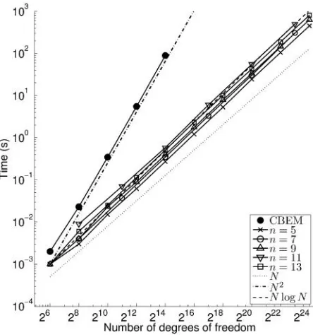
elements, as indicated in the horizontal axes of Figs. 9 and 10. In Fig. 9 are plotted the execution times for the evaluation of Eq. (5) for the analytical values of potentials d and normal gradients t, as implemented
in a C++ code and running on a desktop computer (i7-4770 CPU 3.4GHz, 16GB RAM in Windows 7) for this and all subsequent examples. For the sake of comparison, the execution time required for evaluating Eq. (5) in the frame of the conventional BEM is also plotted (represented by full circles in this and all successive graphs) and shown to be proportional to
N2 (dash-dot line). The remaining plots in Fig. 9 give
the execution time of Eq. (5) for the field poles successively expanded with number of children nc = 2 and the number n of terms in the series of Eq. (1) varying from 5 to 13. The results are in all cases quite the same and shown to be rather proportional to N (dotted line) than to N log N (dashed line), according to the plots. The graphs in Fig. 10 show the Euclidean error norm
/
Hd Gt Gt (13)
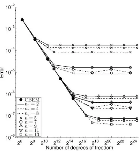
for evaluations carried out combining different children poles nc = 2, 4, 8 and different expansion terms n, also comparing with results of the CBEM. The accuracy tends to increase with nc mainly because the number of adjacent elements to a given element
– for which no series expansion is carried out – also Fig. 8: Square domain for a first simple assessment
[image:7.612.321.543.87.324.2] [image:7.612.67.294.541.724.2]increases with nc. Although the accuracy always increases with n, there is also always a threshold for the mesh refinement.
Irregularly-Shaped Domain with Piece-Wise Straight Boundary
The irregularly-shaped domain of Fig. 11 (Peixoto and Dumont, 2016) is built up with 16 straight segments, which then undergo successive splitting (always keeping the original geometry) in terms of either constant, linear of quadratic elements with up to N = 224 = 16,777,216 degrees of freedom for a potential
problem analysis. This irregularly-shaped domain is submitted to a potential field x2 – y2, with
corresponding nodal potentials d and normal gradients
t evaluated for the numerical accuracy analysis of
the conventional BEM Eq. (5) in terms of FMM expansions. Owing to the polynomial characteristics of the applied potential together with the large domain size and the irregular boundary, the proposed problem actually poses a good challenge to the numerical simulation.
Figure 12 shows the computational times required for constant, linear and quadratic elements
Fig. 10: Accuracy results for different numbers of children poles and expansion terms in the evaluation of Eq. for a linear potential problem over the square of Fig. 8
Fig. 11: Irregularly-shaped domain with the boundary given by piece-wise straight segments
Fig. 12: Execution times for the irregularly-shaped domainof Fig. 11 with nc = 2 children pole expansions
using n = 5, 9, 11, 13 expansion terms and nc = 2 children poles. The running times are all proportional to a function between N and N log N, as in the previous example. The most time expensive case of all did not require more than 15 minutes to run, in the case of
constant elements – and about ten times that for
[image:8.612.317.550.79.561.2] [image:8.612.69.298.80.327.2] [image:8.612.318.548.84.276.2] [image:8.612.321.550.310.549.2]circles), which are proportional to N2, required over a
day of computation for just 216 = 65,536 degrees of
freedom.
A convergence analysis using the Euclidean norm of Eq. (13) is shown in Fig. 13 for all cases discussed with regard to Fig. 11 and also using the results with the conventional BEM for comparison.
Owing to the applied quadratic potential field and the piece-wise straight boundary, the results for quadratic elements should be accurate up to the implemented numerical integration precision of the
conventional BEM – and taking round-off errors into
account. Then, the errors shown for the FMM using quadratic elements are exclusively related to the expansion approximations. In fact, except for some round-off errors, the error diagrams for quadratic elements are horizontal and serve as thresholds for the simulations with constant and linear elements.
An Isolated Assessment for Quadratic Elements
For the domain in Fig. 14, only quadratic elements are used in order to have a cleaner display of results. This structure is discretized with up to N = 5 x 218 =
1,310,720 degrees of freedom and is submitted to a
logarithmic potential field
ln
z
z
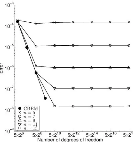
s , where z = x +iy is the field point of the domain, and zs = 12.5 + 15i is the source point, represented by (*) in Fig. 14. The execution time and error results are given in Figs. 15 and 16 as outlined for the previous examples and in the case of nc = 2 children poles. A similar simulation with a larger number of degrees of freedom has already been explored by Peixoto and Dumont (2016).
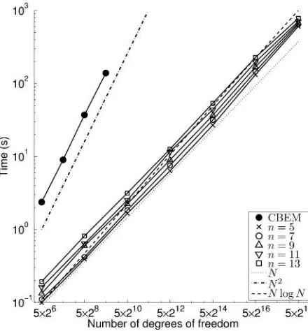
As already observed, one sees in Fig. 15 that the computational effort increases only slightly with
Fig. 13: Accuracy results for the irregularly-shaped domain of Fig. 11 with nc = 2 children pole expansions
Fig. 14: Irregularly shaped domain for an isolated assessment with quadratic elements
[image:9.612.69.294.81.316.2] [image:9.612.318.547.82.280.2] [image:9.612.321.541.473.710.2]the number n of expansion terms. This graph also displays the curves proportional to N (dotted line), N log N (dashed line), and N2 (dash-dot line), which
shows that the present FMM implementation performs close to N, as already suggested by (Liu, 2009) as an achievable goal.
According to Fig. 15, about three seconds were required for achieving an error 10–8, according to
Eq. (13), in the frame of the FMM with N = 5 x 210 =
5,120 degrees of freedom and using n = 13 expansion terms, as given in Fig. 16. Over 15 minutes would be required to obtain the same results with the conventional BEM!
The core of the proposed fast-multipole methodology consists in implementing Eqs. (1)-(4), as applied to the matrix-vector products of the boundary element Eq. (5), in terms of a recursive procedure that scans the field elements hierarchically. Once the most refined level is achieved from a given
superelement, the procedure scans back – also recursively and hierarchically – the whole tree of
superelements inside superelements in search of all source poles and nodal points (Novelino, 2015; Peixoto
et al., 2015, 2015a) in order to build up fast and
efficiently the required matrix-vector products.
The numerical assessments show that the proposed algorithm is seamlessly applicable to generally curved elements of any order, although numerical examples are displayed only for constant, linear and quadratic elements. The simulation of extremely convoluted shapes including multiply-connected domains presents no difficulties. The computational costs for all examples run so far have shown to be closely proportional to O(N) (order of the number of degrees of freedom), as opposed to a conventional BEM implementation, which requires operations of order O(N2). As a matter of fact, the
proposed FMM implementation is superior to a conventional BEM implementation in terms of computational costs even for just a few tens of degrees of freedom, as observed in Figs. 9, 12 and 15.
The proposed FMM has not yet been implemented in an iterative solver, such as the GMRES, since this should be considered as the last step in the developments. In fact, issues such as preconditioning and numerical convergence of the iterative solver itself would only obscure the type of analyses presented in this paper.
Future developments concerning the proposed FMM aim at a three-dimensional formulation and implementation as well as the application to the variationally-based, hybrid boundary element method. Preliminary tests have shown that applications to problems with very complicated fundamental solutions, such as in fracture mechanics (Dumont and Mamani, 2011), may become advantageous regardless of problem size.
Acknowledgements
This work was supported by the Brazilian agencies CAPES, CNPq and FAPERJ.
Fig. 16: Accuracy results for the domain of Fig. 17 using quadratic elements
Conclusion
[image:10.612.70.289.268.503.2]References
Brebbia C A, Telles J C F and Wrobel L C (1984) Boundary
Element Techniques Springer Berlin Heidelberg
Dumont N A (2010) The boundary element method revisited Boundary elements and other mesh reduction methods XXXII 227-238 WITPress, Southampton.
Dumont N A (2012) Unified algorithm for the generation of refined
2D boundary meshes of linear, quadratic and cubic elements Draft paper, PUC-Rio, Brazil
Dumont N A and Aguilar C A (2011) Three-dimensional
implementation of the expedite boundary element method
In extended abstracts of the IABEM2011, symposium of the international association for boundary element methods 113-118, Brescia, Italy
Dumont N A and Aguilar C A (2012) The best of two worlds: The expedite boundary element method Engineering Structures
43 235-244
Dumont N A and Mamani E Y (2011) Generalized Westergaard stress functions as fundamental solutions Computer
Modeling in Engineering and Sciences (CMES) 78
109-149
Dumont N A and Peixoto H F C (2014) Application of the hybrid boundary element method to large-scale problems using a fast multipole technique. 6 pp on CD, PACAM XIV
-14th Pan-American Congress of Applied Mechanics
Greengard L and Rokhlin V (1987) A fast algorithm for particle simulations Journal of Computational Physics 73 325-348
Liu Y (2009) Fast Multipole Boundary Element Method: Theory
and Applications in Engineering Cambridge: Cambridge
University Press
Liu Y J and Nishimura N (2006) The fast multipole boundary element method for potential problems: A tutorial
Engineering Analysis with Boundary Elements 30 371-381
Nishimura N (2002) Fast multipole accelerated boundary integral equation methods Applied Mechanics Reviews 55 299
Novelino L S (2015) A novel fast multipole technique in the
boundary element methods Msc Thesis - PUC-Rio
Peixoto H F C (2014) Application of the hybrid boundary element
method to large-scale problems using fast multipole techniques Msc Thesis - PUC-Rio
Peixoto H F C and Dumont N A (2016) A kernel-independent fast
multipole technique for the analysis of problems with the boundary element method 8 pp, XII Simpósio de Mecânica
Computacional, Diamantina, Brazil
Peixoto H F C, Novelino L S and Dumont N A (2015) Basics of a
fast-multipole unified technique for the analysis of several classes of continuum mechanics problems with the boundary element method 47-59 Boundary Elements and Other Mesh
Reduction Methods XXXVIII, WITPress Southampton
Peixoto H F C, Novelino L S and Dumont N A (2015a) A
fast-multipole unified technique for the analysis of continuum mechanics problems with the boundary element methods12
pp, CILAMCE – XXXVI Iberian Latin-American