A Bayesian approach for correcting bias of data envelopment analysis estimators

Munich Personal RePEc Archive

A Bayesian approach for correcting bias

of data envelopment analysis estimators

Zervopoulos, Panagiotis and Emrouznejad, Ali and Sklavos,

Sokratis

Department of Management, University of Sharjah, Operations

Information Management Department, Aston Business School,

NeuroBioAnalysis Lab

January 2019

Online at

https://mpra.ub.uni-muenchen.de/91886/

A Bayesian approach for correcting bias of data envelopment analysis estimators

Panagiotis D. Zervopoulos*

Department of Management

University of Sharjah, Sharjah 27272, United Arab Emirates

Tel.: +971 567159809

[email protected]

Ali Emrouznejad

Operations & Information Management Department

Aston Business School, Aston University, Birmingham B4 7ET, UK

[email protected]

Sokratis Sklavos

NeuroBioAnalysis Lab, 2 Lefktron St & Michalakopoulou Av., Athens 11527, Greece

[email protected]

*_{Corresponding author}

Abstract

The validity of data envelopment analysis (DEA) efficiency estimators depends on the

robustness of the production frontier to measurement errors, specification errors and

the dimension of the input-output space. It has been proven that DEA estimators, within

the interval (0, 1], are overestimated when finite samples are used while asymptotically

this bias reduces to zero. The non-parametric literature dealing with bias correction of

efficiencies solely refers to estimators that do not exceed one. We prove that efficiency

estimators, both lower and higher than one, are biased. A Bayesian DEA method is

developed to correct bias of efficiency estimators. This is a two-stage procedure of

super-efficiency DEA followed by a Bayesian approach relying on consistent efficiency

estimators. This method is applicable to ‘small’ and ‘medium’ samples. The new

Bayesian DEA method is applied to two data sets of 50 and 100 E.U. banks. The mean

square error, root mean square error and mean absolute error of the new method reduce

Keywords: Data envelopment analysis; Super-efficiency; Bayesian methods; Statistical

inference; Banking

1. Introduction

Data envelopment analysis (DEA) put forth by Charnes et al. (1978) and extended by

Banker et al. (1984) is a mathematical programming methodology to evaluate the

efficiency of a sample firm relative to a reference set of all sample firms. DEA is a

non-parametric approach to construct production frontiers based on observed input and

output data of the sample firms. Despite the non-parametric nature of DEA, Banker and

Maindiratta (1992), Banker (1993), Sarath and Maindiratta (1997), Banker and

Natarajan (2008) provided statistical justification for DEA. In particular, Banker (1993)

proved that DEA (with one output and multiple inputs), under the conditions of

monotonicity and concavity, yields consistent estimators of the production frontier. The

studies of Simar and Wilson (1998, 1999), Kneip et al. (2008, 2011), Kuosmanen and

Johnson (2010) and Tsionas and Papadakis (2010) also allowed for inference on DEA

efficiency estimators.

The validity of DEA efficiency estimators depends on the robustness of the production

frontier to measurement errors, specification errors and the dimension of the

input-output space. Banker (1993) was the first to highlight the overestimation of DEA

efficiencies when finite samples are used. Banker (1993) and Grosskopf (1996) showed

that this bias asymptotically reduces to zero. In line with these studies, Simar (2007)

identified an inverse relationship between the rate of convergence of DEA efficiency

estimators and the dimensionality of the production set. Simar and Wilson (2015) stated

that the true efficiency of a firm is unknown.

Emphasizing DEA, there are six major approaches dealing with the sensitivity of

efficiency estimators: (a) Chance Constrained DEA (CCDEA); (b) Two-stage

DEA-based methods; (c) Corrected Concave Non-Parametric Least Squares (C2NLS); (d)

Stochastic Non-Smooth Envelopment of Data (StoNED); (e) Bayesian DEA; and (f)

CCDEA (Charnes and Cooper, 1963; Land et al., 1993; Olesen and Petersen, 1995)

specifies stochastic production frontiers by replacing the observed input and output data

with their randomly distributed counterparts. CCDEA programs are appropriate for

dealing with the presence of noise in the data. However, they lack statistical theory. A

review of CCDEA is available in Olesen and Petersen (2016). Two-stage DEA-based

procedures presented by Banker and Natarajan (2008) for estimating non-parametric

stochastic frontiers. In the first stage, a conventional DEA model is applied (e.g. the

variable returns to scale (VRS) DEA put forth by Banker et al. (1984)) to estimate the

technical efficiency of sample firms. In the second stage, the DEA efficiency estimators

obtained from the previous stage are introduced in OLS and maximum likelihood

models to yield consistent estimators.

The C2NLS (Kuosmanen and Johnson, 2010) is a least-square interpretation of the VRS

DEA model, which, in contrast to conventional DEA models constructing production

frontiers based on dominant firms, uses all available information for estimating a

production frontier. Kuosmanen and Johnson (2010) concluded that the C2NLS

estimators outperform DEA estimators when the number of firms are significantly

higher than the number of input and output variables while the C2NLS estimators

perform at least as well as the DEA estimators when dimensionality is present. The

StoNED method (Kuosmanen and Kortelainen, 2007; Kuosmanen and Kortelainen,

2012) estimates semiparametric frontiers by combining the DEA-style frontier with the

Stochastic Frontier Analysis (SFA)-style treatment of inefficiency and noise. StoNED

facilitates statistical inference while relying on regularity properties (e.g. free

disposability, convexity) and without requiring the assumption of a particular

production function.

A Bayesian DEA approach for CCDEA was developed by Tsionas and Papadakis

(2010). This method provides statistical inference (e.g. estimation of CCDEA

efficiencies based on an estimated prior distribution, construction of confidence

intervals) to CCDEA relying on assumptions about the distribution (e.g. multivariate

normal) of the (posterior/observed) inputs and outputs. Relying on the distribution of

the posterior input and output data, it is possible to estimate the prior distribution of the

data and then estimate CCDEA efficiencies. This approach lacks formal statistical

Bootstrap DEA is a widely used method for correcting bias and constructing confidence

intervals of efficiency estimators (Kneip et al., 2008). Bootstrap DEA, or smoothed

bootstrap, originated from Simar and Wilson (1998), combines both the virtues and

limitations of bootstrap and DEA. Smoothed bootstrap relies on pseudo-data obtained

from an estimated data generating process (DGP) (Dyson and Shale, 2010). Kneip et

al. (2008, 2011) developed improved smoothed bootstrap algorithms providing

consistent bias-corrected estimators. Major limitations of the smoothed bootstrap are

the considerably large confidence intervals, which make difficult to obtain meaningful

comparisons between the sample firms, and unsatisfactory performance when

inadequate samples for the dimension of the input-output space are available.

All methods discussed above dealing with the sensitivity of DEA efficiencies refer to

estimators lying within the interval (0, 1]. Andersen and Petersen (1993), drawing on

the work of Banker and Gifford (1988), presented a super-efficiency DEA model,

which makes possible efficiency estimators to exceed unity, unlike the conventional

DEA models, as the firm under review is excluded from its own reference set.

Super-efficiency DEA procedure is used for ranking efficient units and identifying outliers

(Banker and Chang, 2006). However, Banker and Chang (2006) and Banker et al.

(2017) found that super-efficiency performs unsatisfactorily in ranking efficiency units.

It should be noted that this result has not been tested to cases of multiple inputs and

multiple outputs and input values considerably greater than 20. Another issue of the

traditional super-efficiency DEA model under VRS is the infeasibility.

The contribution of this work is to provide statistical inference in super-efficiency DEA

models. We develop a two-stage Bayesian DEA approach to correct bias of

super-efficiency estimators. In the first stage, we use a super-super-efficiency DEA model while in

the second stage we specify consistent super-efficiency estimators. These estimators

are introduced in the Bayesian framework to estimate bias-corrected (prior)

super-efficiencies. To the best of our knowledge, this is the first work on correction of bias of

super-efficiency estimators.

The rest of the paper unfolds as follows. In Section 2, we present the super-efficiency

conventional statistical inference; Step 2: Bayesian statistical inference; Step 3: bias

correction). In Section 3, we present the two data sets used in this study and analyze the

results. Section 4 concludes and discusses future research directions.

2. Methodology

2.1 Super-efficiency DEA

After the work of Andersen and Petersen (1993), many studies appear in the literature

(Lovell and Rouse, 2003; Chen, 2005; Li et al., 2007; Ray, 2008; Cook et al., 2009;

Chen et al., 2011; Lee et al., 2011; Chen and Liang, 2011) dealing with the

measurement of super-efficiency in DEA under the condition of VRS. The latter studies

tried to solve the problem of infeasibility of the VRS super-efficiency DEA model.

In this study, we use Chen and Liang (2011)’s model to obtain super-efficiency

estimators (_j), which is as follows

1

min

s r r

M

 

  



1

. . (1 ) 1, 2,...,

n

j ij io j

j o

s t  x  x i m

 

  



1

(1 ) 1, 2,...,

n

j rj r ro j

j o

y y r s

 

 

  



1

1

n j j j o

  





_j 0, jo, _r 0 (1)

where M is a user-defined large positive number (e.g. 105).

The super-efficiency estimators are defined as 1 1 1 1 r R

r

R



   





For the application of this Bayesian DEA method for the correction of bias of the

super-efficiency DEA estimators, other super-super-efficiency models (e.g. Chen, 2005; Li et al.,

2007; Ray, 2008; Cook et al., 2009; Chen et al., 2011; Lee et al., 2011) can be used

instead of model (1).

2.2 Conventional statistical inference

Let  (j), where j 0 (j1, 2,..., )n , be a random variable of independently and identically distributed (iid) super-efficiency estimators obtained from model (1).  is assumed uniformly distributed from _L (0_L1) to  _U ( U 1). The two parameters (i.e. _L and _U) are unknown.

Acknowledging the probability density function (PDF) of  as 1

,

( , )

0 , otherwise

L j L

j L

f_        

 _{ }

   



U U

U (2)

the likelihood function is expressed as follows

iid

1

1

( , ) ( , ) , , 1, 2,...,

( )

n

L U j L U n L j U

j U L

L   f       j n

 

 

     





By partially differentiating the likelihood function (3)

1

1

( , ) 0

( )

( , ) 0

( )

L n

L L

L n

U L

n L

n L

 

  

 

  





 _{  }

 

 _{   }

 

U

U

U

U

we find that it is monotone increasing for _L and monotone decreasing for U. Hence,

the likelihood function (3) is maximized at ˆL min and ˆU max.

Taking into account the maximum likelihood estimators (MLE) ˆL and ˆU, we define the joint cumulative distribution function (CDF) as follows

ˆ ˆ

( _L,_U)( , ) Prob(ˆL , ˆU ) Prob(min , max )

F_{ } t s   t  s   t  s





iid

1 1

Prob(max  s) Prob( s,...,_n  s) Prob( s) n

1 1

= ( , )d

L n s L U f               



d , 1

L

n _n

s

L

U

U L U L

s s           _{  }   _{ } _{ }    _  _  





and





iid

1 1

Prob(min t, max  s) Prob(t s,...,t_n  s) Prob(t s) n

1 1 1

1 ( , )d d

n n

s s

L U

U L

t t

f     

       _{ } _{ }  





  (6)

Based on expressions (4)-(6), the joint CDF is written as follows

ˆ ˆ

( L,U)( , , ) ,

n n

L

L U L U

U L U L

s s t

F_{ } t s    t s 

   

     

_{ } _{ }   

 

    (7)

with corresponding joint PDF

2

ˆ ˆ ˆ ˆ ˆ ˆ

( _L,_U)( , L, U) ( _L,_U)( , ) ( _L,_U)( , )

f t s F t s F t s

t s t s

              _{ }      1 1 ( ) ( ) ( ) ( ) n n L n n

U L U L

n s n s t

t              _  _  _   _ 2

( 1)( ) , ( ) n L U n U L

n n s t

t s           

 (8)

The marginal PDF of ˆL is expressed as follows

2

ˆ (ˆ ˆ, )

( 1)( )

( , ) ( , , )d d

( )

U U

L L U

n

L U L U n

U L

t t

n n s t

f t f t s s s

         _{ }      





U L U

n U L n t t          

 (9)

and the corresponding marginal PDF of ˆ_U reads as follows

2

ˆ (ˆ ˆ, )

( 1)( )

( , ) ( , , )d d

( )

U L U

L L

s s n

L U L U n

U L

n n s t

f_ s f_{ } t s t t

1

( ) ,

( )

n

L L U

n U L

n

s   s 

 



   

 (10)

As we noticed in expressions (8)-(10)

ˆ ˆ ˆ ˆ

(_L,_U)( , L, U) _L( L, U) _U( L, U)

f_{ } t s   f_ t  f_ s  (11)

Hence, the MLE ˆL and ˆU are not independent.

The expected value of ˆ_L is (see Appendix 1.1 for formal mathematical analysis)

 

1

ˆ _{( , )d 1}

1 1

U

L L

n L L U L U

n

E t f t t

n n

  

       

 



Based on (12), we conclude that the MLE ˆL is asymptotically unbiased to the

parameter L as lim n

 

nE   (13)

The second moment of ˆ_L is defined as follows (see Appendix 1.2 for formal mathematical analysis)

 

ˆ 2( ) ( 1)

ˆ _{( , )d}

1 2

U

L L

U L L U

n L L U L

n

E t f t t

n n

  

   

          

 



In addition, the variance of ˆ_L is

     

Varn L En L En L

2

2 2( ) ( 1) 1

1 2 1 1

U L L U

L L U

n n

n n n n

   

      

   _  _

      (15)

It is straightforward that lim Var_n

 

n   . (16)

The mean square error (MSE) of ˆ_L is

 

 

 

MSE_n _L bias_n _L Var_n _L (17)

   

biasn L En L L (18)

The MLE ˆL is a consistent estimator of the parameter L.

Proof. Based on expression (13) and (16), we find that lim bias_n

 

n   and

 

lim MSE_{n L} 0

n   .

Likewise, the expected value of ˆ_U is (the formal mathematical analysis is like that in Appendix 1.1)

 

1

ˆ _{( , )d}

1 1

U

U L

n U L U U L

n

E s f s s

n n

  

      

 



where 1 1 L U

n



    to ensure that the mean value of ˆ_U is always greater than unity.

Based on expression (19), we conclude that the MLE ˆ_U is asymptotically unbiased to

the parameter U as lim n

 

nE   . (20)

The second moment of ˆ_U is defined as follows (the formal mathematical analysis is like that in Appendix 1.2)

 

ˆ 2( ) ( 1)

ˆ _{( , )d}

1 2

U

U L

U L U L

n U L U U

n

E s f s s

n n

  

   

          

 



and its variance is

     

Varn U En U En U

2

2 2( ) ( 1) 1

1 2 1 1

U L U L

U U L

n n

n n n n

   

      

   _  _

      (22)

It is straightforward that lim Varn

 

n   . (23)

The MSE of ˆ_U is

 

 

 

and the bias is defined as follows

   

biasn U En U U (25)

The MLE ˆ_U is consistent estimator of the parameter U .

Proof. Based on expressions (20) and (23), we find that lim biasn

 

n   and

 

lim MSE_{n U} 0

n   .

Using expressions (12) and (19), the unbiased estimators of parameters _L and _U are

ˆ ˆ _ˆ

1 L U

L L

n n

 

   

 (26) and,

ˆ ˆ _ˆ

1 U L

U U

n n

 

   

 (27) respectively, which satisfy

 

n L L

E   (28) and E_n

 

The covariance of ˆ_L and ˆ_U is defined as follows (see Appendix 2 for formal mathematical analysis)

     

ˆ ˆ ˆ ˆ ˆ ˆ

cov (n  L, U)En  L U En L En U

2 2 2 2

2

( ) ( 1) ( )

2 ( 1)

U L L U L U

L U

n n

n n

     

     

  

  (30)

The covariance of ˆL and ˆU facilitates the definition of the variance of the unbiased

estimator _L. Using property (26), the variance is

 

Var Var

1

L U

n L n

n n

    _  _



 

 

 

 





2

1 _{ˆ ˆ ˆ ˆ}

Var Var 2 cov ( , )

(n 1) n n L n U n n  L U

  

 (31)

which is asymptotically zero, lim Var_n

 

n   (32)

In addition, MSE_n

 

 

Proof. Based on expressions (28) and (32), we find that lim MSE_n

 

n   .

Likewise, using property (27), the variance of the unbiased estimator _U is

 

Var Var

1

U L

n U n

n n

    _  _



 

 

 

 









2

1 _{ˆ ˆ ˆ ˆ}

Var Var 2 cov ,

(n 1) n n U n L n n  L U

  

 (34)

which is asymptotically zero lim Var_n

 

n   (35)

and MSE_n

 

 

The unbiased estimator _U is consistent to parameter _U.

Proof. Expressions (29) and (35) lead to lim MSEn

 

n   .

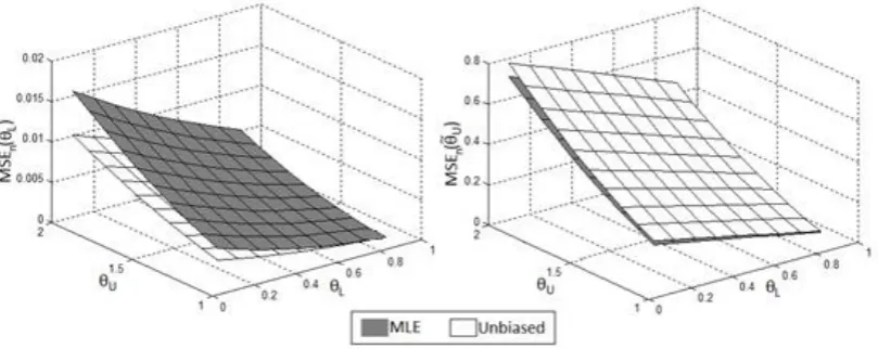
Figure 1 illustrates the performance of the MSE of the unbiased estimators against that

of the maximum likelihood estimators. This comparative analysis is obtained from

1,000 Monte Carlo simulations. In detail, we find that MSEn

 

 

 

 

MSEn U MSEn U . Therefore, the unbiased estimator L is better than the

corresponding MLE ˆ_L for the parameter _L while the opposite applies for the parameter _U.

The covariance of L and U is defined as follows (see Appendix 3 for formal mathematical analysis)

     

cov (n  L, U)En  L U En L En U

2 2 2

2

2 2

2 2

( ) 2( )

1

( 1) 2 ( 1) ( 1)

U L U L

L U L U L U

n n

n n n n

   

     

     



 _  _ _   _

 _  _  _  _ (37)

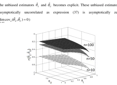
Based on expression (37) we develop Figure 2 where an inverse relationship between

the unbiased estimators L and U becomes explicit. These unbiased estimators are asymptotically uncorrelated as expression (37) is asymptotically zero (

lim cov (n L, U) 0 n    )

Figure 2. Covariance of the unbiased estimators _L and _U

2.3 Bayesian statistical inference

The prior

Let the vector    ( _O, _I) of super-efficiency scores where  _O (₁,...,_k),

O 1

L

    , and  _I (_k1,...,_n), 1  _I _U. In the absence of any information

about the distribution of the DEA super-efficiency scores, we assume _O_L and

I U

O

1

, 1, 1,..., 1

( )

0 , otherwise

L j L

j L

j k

f_     

 _{  }

   

 (38)

I

1

, 1 , 1,...,

1

( )

0 , otherwise

j U U

j U

j k n

f_     

 _{   }

 _  

 (39)

and joint PDF

O O iid O 1 1 ( ) ( ) (1 ) k

L j L k

j L

f  f  



 



  





I I iid I 1 1 ( ) ( ) ( 1) n

U j U n k

j k U

f  f  

 

 

 

  





The parameter _L could be beta-distributed (see Appendix 4) with parameters  0 and  0.

Assuming the unbiased estimator of _L is equivalent to the expected value of the prior

beta distribution of _L (i.e. 

  ), we find that δ is an expression of γ

(1 _L)

L

  





 (42)

and the prior beta distribution is reduced to the single parameter γ.

The vector O has a joint PDF

O O

1

O O

0

( , )

( ) ( ) ( )d

( , )

L

L L L L

k

f f _  f_    

 

 

 

   





where  k (beta function is defined in Appendix 4).

Then, the parameter γ is lower bounded

1 L L k    

 (44)

Assuming the unbiased estimator is identical to the expected value 1 of the prior shifted gamma-distribution of _U, then the parameter  is an expression of 

1

U

 





 (45)

Hence, the prior shifted gamma-distribution is reduced to the single parameter  .

The vector _I has a joint PDF

I I I I

1

( )

( ) ( ) ( )d

( )

U

U U U U

n k

f f _  f_   





 

  

   





where  n k.

Then, the parameter  is upper bounded U 1

n k

   

 (47)

The posterior

The Bayesian PDF of _L _O is Ο

Ο

Ο Ο Ο

Ο

( ) ( )

( )

( )

L L

L L

L

f f

f

f

 

 

 



   

 (48)

According to the joint PDF (40), the Bayesian PDF (48) becomes

1 ( ) 1

1

(1 )

( , )

k

L L

k

     

 _  

  (49)

which refers to a posterior beta distribution with parameters  and k .

The posterior beta distribution shifts the corresponding prior beta distribution, with

parameters  and  , to the right, which is justified by the following expected values





 

k L k L

E   E  as

k

 

     (50)

I I

I

1

I I

I

1

( 1) exp

( ) ( )

( )

( ) ( )

U U

n k U

U

U U

U n k

f f

f

f n k

 

 

 

  _



 

   

  



  

 _ _

 _{ }

  

    (51)

which refers to a posterior shifted gamma distribution with parameters   n k 0 and  0.

The posterior shifted gamma distribution shifts the corresponding prior distribution to

the left, which justifies the underestimation of the DEA efficiencies that are greater than

one. This underestimation is explained as follows





 

n k U n k U

E _   E _  as ( n k) 1 1 (52)

2.4 Bias correction

Let a correction parameter L  L/ ˆL where L 1 (53)

Elaborating on expressions (42), (44) and (53), we estimate parameters  and  as follows

ˆ k _L/ (1 _L)

    (54)

and ˆ (1 L)ˆ L

  





 (55)

Two random data sets of size k are generated, where k expresses the number of DMUs

assigned efficiencies (e.g. obtained from DEA program (1)) lower than unity. The first

randomly generated data set is drawn from a prior beta distribution of _L with

parameters ˆ and ˆ (see expressions (54) and (55)). The second randomly generated

data set is drawn from a posterior beta distribution _L _O with parameters ˆ and ˆk

. The prior to posterior distribution

O

L L

L

   

 is fitted by a gamma distribution with

parameters z_O 0 and e_O 0. The maximum likelihood estimates of these two

parameters (i.e. zˆ_O and eˆ_O) are obtained from the MATLAB function gamfit. The

The corrected estimator is

O ˆO

ˆ

( , )

p pGamma z e

  , p1,..., (k p j) (56)

with confidence interval _p s( p)cv _{p p} s( p)cv

w w

 

     (57)

where w expresses the number of Monte Carlo iterations and cv denotes the critical

value of t-distribution with w1 degrees of freedom.

The Monte Carlo simulated mean and standard deviation are defined as follows

1 , 1

w

p p l

l

w

  







and 1 2

, 1

( ) ( 1) ( )

w

p p l p

l

s w   



 



With respect to the DEA estimators that are greater than unity, we define a correction

parameter U  U / ˆU that satisfies U 1 (60)

We already know that   n k (46) and  u 1





 (45). To estimate the two

parameters of the shifted gamma distribution we introduce ( _ˆ1) 1

( )

U U U

  

 _

 in (46), which

leads to ˆ ( )( _ˆ 1)

( )

U U U

n k 



 

 



 (61) and

1

ˆ ˆ U

 





 (62).

Similar to the correction process followed for the DEA estimators lying within the

interval (0,1), for the estimators exceeding one, we generate two random data sets for

both the prior shifted gamma distribution with parameters ˆ and ˆ, and the posterior shifted gamma distribution with parameters ˆ n k and ˆ. The prior to posterior

distribution

I

U U

U

   

 is fitted by a gamma distribution with parameters zI 0 and

I 0

obtained from the MATLAB function gamfit. Like above, the goodness-of-fit is

calculated using the Wilcoxon rank sum test for equal medians.

The corrected estimator is

I ˆI

ˆ

( , ) q qGamma z e

  , q1,...,n k (q j) (63)

with confidence interval _q s( q)cv _{q q} s( q)cv

w w

 

     (64)

where 1 _,

1

w

q q l

l

w

  







1

( ) ( 1) ( )

w

q q l q

l

s w   



 



3. Application to E.U. banks

3.1 Data set and selection of variables

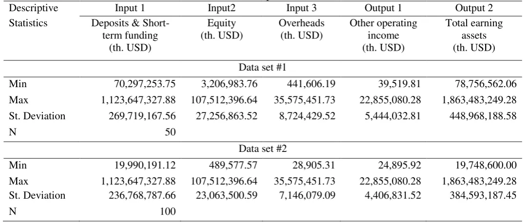
In this study, we used two data sets to test the performance of the Bayesian DEA method

in correcting bias of DEA estimators. The first data set consists of 50 banks while the

second one is expanded to 100 banks. In practice, the second data set includes 50 new

banks in addition to those of the first data set. Both data sets include three inputs (i.e.

(a) Deposits & Short-term funding; (b) Equity; (c) Overheads) and two outputs (i.e. (a)

Other operating income; (b) Total earning assets). The data come from Orbis Bank

Focus (the two data sets are available in the online version of this article; see Table E1).

The size of both samples is considered adequate for the dimension of the input-output

space. The sample size (e.g. 50 banks) satisfies the ‘rule of thumb’ put forth by Cooper

et al. (2007): nmax{xy, 3(xy)}, where n stands for the number of firms and x and

y are the number of inputs and output, respectively. However, the DEA efficiency

estimators assigned to the banks are expected to be biased as the samples of 50 and 100

firms are regarded as small and medium (Banker et al., 2010).

Descriptive statistics of the two-real-world data sets we used in this study are presented

Table 1. Descriptive statistics

Descriptive Input 1 Input2 Input 3 Output 1 Output 2 Statistics Deposits & Short-

term funding (th. USD)

Equity (th. USD)

Overheads (th. USD)

Other operating income (th. USD)

Total earning assets (th. USD) Data set #1

Min 70,297,253.75 3,206,983.76 441,606.19 39,519.81 78,756,562.06 Max 1,123,647,327.88 107,512,396.64 35,575,451.73 22,855,080.28 1,863,483,249.28 St. Deviation 269,719,167.56 27,256,863.52 8,724,429.52 5,444,032.81 448,968,188.58

N 50

Data set #2

Min 19,990,191.12 489,577.57 28,905.31 24,895.92 19,748,600.00 Max 1,123,647,327.88 107,512,396.64 35,575,451.73 22,855,080.28 1,863,483,249.28 St. Deviation 236,768,787.66 23,063,500.59 7,146,079.09 4,406,831.52 384,593,187.45

N 100

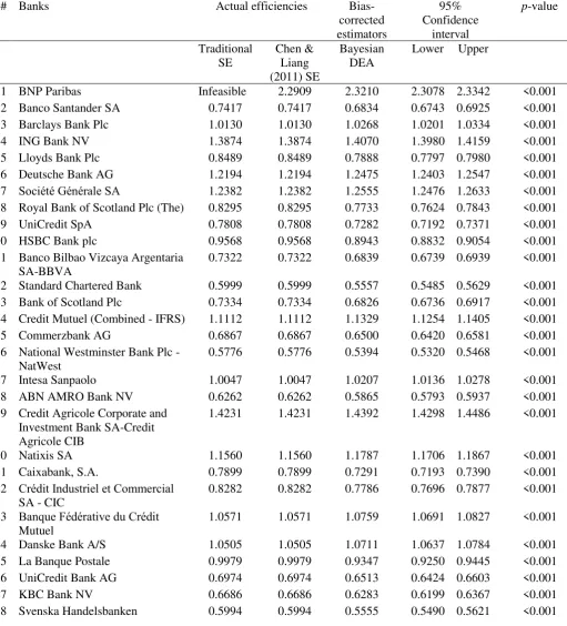
3.2 Empirical results

The empirical results of the first data set, consisting of 50 banks, are reported in Table

2. The actual efficiencies refer to the results obtained from the traditional

super-efficiency model of Andersen and Petersen (1993) and Chen and Liang (2011)’s super

-efficiency model (see model (1)). The bias-corrected super--efficiency estimators

yielded by our Bayesian DEA approach are presented on the right side column of the

actual efficiencies followed by the 95% Monte Carlo confidence intervals of the

bias-corrected estimators and the significance of the bias correction process (p-value).

According to Table 2, the Bayesian DEA approach presented in Section 2 yields

reduced estimators for actual efficiencies lower than one and increased estimators for

actual efficiencies exceeding one. The mean bias of efficiency estimators below one is

higher (i.e. mean bias: -0.0533; min bias: -0.0325 and max bias: -0.0723) than the bias

of the estimators above one (i.e. mean bias: 0.0209; min bias: 0.0137 and max bias:

0.0363). Moreover, in the case of estimators below one, the bias is higher for those

getting closer to unity while lower for the estimators with higher deviation from one.

The opposite applies to the super-efficiency estimators as the bias becomes lower when

the estimator approaches one and higher when it moves far from one. All bias-corrected

In the case of the sample of 50 banks, the mean square error (MSE), root mean square

error (RMSE) and mean absolute error (MAE) of the Bayesian DEA estimators are

0.0021, 0.0453 and 0.0416, respectively.

Table 2. Empirical results

# Banks Actual efficiencies

Bias-corrected estimators

95% Confidence

interval

p-value

Traditional SE

Chen & Liang (2011) SE

Bayesian DEA

Lower Upper

1 BNP Paribas Infeasible 2.2909 2.3210 2.3078 2.3342 <0.001 2 Banco Santander SA 0.7417 0.7417 0.6834 0.6743 0.6925 <0.001 3 Barclays Bank Plc 1.0130 1.0130 1.0268 1.0201 1.0334 <0.001 4 ING Bank NV 1.3874 1.3874 1.4070 1.3980 1.4159 <0.001 5 Lloyds Bank Plc 0.8489 0.8489 0.7888 0.7797 0.7980 <0.001 6 Deutsche Bank AG 1.2194 1.2194 1.2475 1.2403 1.2547 <0.001 7 Société Générale SA 1.2382 1.2382 1.2555 1.2476 1.2633 <0.001 8 Royal Bank of Scotland Plc (The) 0.8295 0.8295 0.7733 0.7624 0.7843 <0.001 9 UniCredit SpA 0.7808 0.7808 0.7282 0.7192 0.7371 <0.001 10 HSBC Bank plc 0.9568 0.9568 0.8943 0.8832 0.9054 <0.001 11 Banco Bilbao Vizcaya Argentaria

SA-BBVA

0.7322 0.7322 0.6839 0.6739 0.6939 <0.001

12 Standard Chartered Bank 0.5999 0.5999 0.5557 0.5485 0.5629 <0.001 13 Bank of Scotland Plc 0.7334 0.7334 0.6826 0.6736 0.6917 <0.001 14 Credit Mutuel (Combined - IFRS) 1.1112 1.1112 1.1329 1.1254 1.1405 <0.001 15 Commerzbank AG 0.6867 0.6867 0.6500 0.6420 0.6581 <0.001 16 National Westminster Bank Plc -

NatWest

0.5776 0.5776 0.5394 0.5320 0.5468 <0.001

17 Intesa Sanpaolo 1.0047 1.0047 1.0207 1.0136 1.0278 <0.001 18 ABN AMRO Bank NV 0.6262 0.6262 0.5865 0.5793 0.5937 <0.001 19 Credit Agricole Corporate and

Investment Bank SA-Credit Agricole CIB

1.4231 1.4231 1.4392 1.4298 1.4486 <0.001

20 Natixis SA 1.1560 1.1560 1.1787 1.1706 1.1867 <0.001 21 Caixabank, S.A. 0.7899 0.7899 0.7291 0.7193 0.7390 <0.001 22 Crédit Industriel et Commercial

SA - CIC

0.8282 0.8282 0.7786 0.7696 0.7877 <0.001

23 Banque Fédérative du Crédit Mutuel

1.0571 1.0571 1.0759 1.0691 1.0827 <0.001

29 Banco de Sabadell SA 0.8004 0.8004 0.7395 0.7303 0.7487 <0.001 30 Bankia, SA 0.5714 0.5714 0.5388 0.5319 0.5458 <0.001 31 UniCredit Bank Austria AG-Bank

Austria

0.7621 0.7621 0.7053 0.6954 0.7151 <0.001

32 Deutsche Postbank AG 0.7525 0.7525 0.7003 0.6919 0.7088 <0.001 33 ING-DiBa AG 0.5462 0.5462 0.5057 0.4987 0.5128 <0.001 34 Skandinaviska Enskilda Banken

AB

1.0449 1.0449 1.0627 1.0556 1.0699 <0.001

35 Banco Popular Espanol SA 0.6505 0.6505 0.6097 0.6017 0.6178 <0.001 36 Le Crédit Lyonnais (LCL) SA 0.8824 0.8824 0.8131 0.8023 0.8239 <0.001 37 ING Belgium SA/NV-ING 0.7142 0.7142 0.6624 0.6545 0.6704 <0.001 38 Banca Monte dei Paschi di Siena

SpA-Gruppo Monte dei Paschi di Siena

1.1716 1.1716 1.1977 1.1896 1.2058 <0.001

39 Deutsche Bank Privat-und Geschaftskunden AG

1.5377 1.5377 1.5564 1.5454 1.5675 <0.001

40 Banco BPM SPA 0.9995 0.9995 0.9390 0.9267 0.9512 <0.001 41 Belfius Banque SA/NV-Belfius

Bank SA/NV

0.8518 0.8518 0.7938 0.7833 0.8043 <0.001

42 Raiffeisen Bank International AG 0.9183 0.9183 0.8549 0.8444 0.8655 <0.001 43 Bank Austria Creditanstalt AG 0.9260 0.9260 0.8624 0.8511 0.8737 <0.001 44 Dexia Crédit Local SA 2.4948 2.4948 2.5311 2.5143 2.5479 <0.001 45 Caixa Geral de Depositos 1.1182 1.1182 1.1368 1.1305 1.1432 <0.001 46 Allied Irish Banks plc 0.9073 0.9073 0.8350 0.8229 0.8471 <0.001 47 Piraeus Bank SA 0.9216 0.9216 0.8615 0.8509 0.8721 <0.001 48 Abbey National Treasury

Services Plc

1.1857 1.1857 1.2032 1.1955 1.2109 <0.001

49 National Bank of Greece SA 0.9647 0.9647 0.8942 0.8826 0.9059 <0.001 50 Deutsche Kreditbank AG (DKB) 1.2066 1.2066 1.2235 1.2147 1.2323 <0.001

MSE 0.0021

RMSE 0.0453

MAE 0.0416

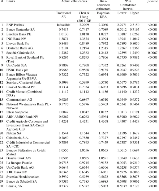
In the case of the extended sample of 100 banks (Table A1 in Appendix 6), the MSE,

RMSE and MAE of the Bayesian DEA estimators are 0.0013, 0.0355 and 0.0321,

respectively. All three measures are lower than the corresponding measures referring

to the sample of 50 banks (Table 2). It should be noted that this Bayesian DEA approach

is appropriate for small and medium samples where the estimators, lower and greater

than unity, are dependent. Based on expression (37) and Figure 2, it is straightforward

4. Concluding remarks and future research

The purpose of this study was to develop a Bayesian DEA approach for correcting bias

of super-efficiency estimators. The new method uses consistent estimators to the

unknown efficiency parameters to correct the bias of the actual efficiencies. The

assumptions made for the development of the Bayesian DEA method are regarded as

realistic.

The new method draws on Chen and Liang (2011)’s super-efficiency model. However,

other super-efficiency models that tackle the infeasibility problem could be used

instead. The new Bayesian DEA method is appropriate for small and medium data sets

where dependence among the estimators below and above one is present. The empirical

results showed a decrease in MSE, RMSE and MAE when the sample size increases.

In addition, the range of the 95% Monte Carlo confidence intervals of the estimators

decreases while the sample size becomes larger. The empirical analysis presented in

this study was based on two real-world data sets of 50 and 100 firms coming from the

E.U. banking sector. The two data sets included three inputs and two outputs.

Further research is needed to test the performance of the new Bayesian DEA

bias-corrected estimators when real-world data sets of different dimensions and scales than

those used in this study are employed. The Bayesian DEA method presented in this

work should be modified to become appropriate for large samples as well. Furthermore,

the application of outlier-detection methods in conjunction with the new Bayesian DEA

method would prevent distortion of the bias-corrected estimators - especially in cases

where observed efficiency estimators are significantly higher than one. Addressing

these limitations would improve the performance, applicability and generalizability of

Appendices

Appendix 1.1

The expected value of ˆ_L is as follows

 

ˆ

1 d

ˆ _{( , )d ( ) d ( ( ) )d}

( ) ( ) d

U U U

L

L L L

n n

n L L U n U n U

U L U L

n

E t f t t t t t t t t

t                          







( ( ) ) 1 1 d ( )

= ( ) d d

( ) ( ) ( ) d 1

U _{U U}

L L L n n n U U U L

n n n

U L U L U L

t t t

t t t

t n  _{ }     _{ }             _{   }      





( ) 1 1

U

L

n

U U L

L n L

U L t n n                      1 1 1 1 L U n n n        Appendix 1.2

The second moment of ˆL is defined as follows

 

ˆ 1

2( ) ( 1)( )

ˆ _{( , )d d}

1 ( )

U U

L

L L

n

U L U

n L L U L n

U L

n t

E t f t t t t

n                          





 

2( ) _ˆ 2( ) ( 1)

1 1 2

U L U L L U

L n L L

n E

n n n

                       Appendix 2

The covariance of ˆ_L and ˆ_U is defined as follows

     

ˆ ˆ ˆ ˆ ˆ ˆ

cov (n  L, U)En  L U En L En U (A2.a)

where

 

ˆ ˆ

( , )

( 1)( )

ˆ ˆ _{( , , )d d d d}

( )

U U

L U

L L L L

s s n

n L U L U n

U L

n n s t

E ts f t s t s ts t s

                   

 

 

( 1)( ) d d

( ) U L L s n n U L n

s t n s t t s



   



  



 

2 1 ( )

( 1)( ) d ( )

L

s n

n n L

L L

s

t n s t t s

n            



2 2

1 ( ) ( ) ( ) ( )

( ) d

( 1) ( 1)( 2)

U

L

n n n

n

n L L U U L U L U L

L L

s

s s s

n n n n n n n

                 _{ }   _  _  _    _{  }  



By replacing (A2.c) and (A2.d) in (A2.b), we obtain

 

( ) ( ) ( )

ˆ ˆ

( ) ( 1) ( 1)( 2)

n n n

U L U L U L

n L U n L U

U L

n E

n n n n n n

                    _   _  _    _ 2 ( ) 2 U L L U n       

 (A2.e)

Introducing expressions (A2.e),

 

1 1

n L L U

n E

n n

  

  (12), and

 

1 1

n U U L

n E

n n

  

  (19) in (A2.a) we find





2

( ) ( 1) ( )

ˆ ˆ

cov ,

2 ( 1)

U L L U L U

n L U L U

n n n n                   Appendix 3

The covariance of _L and _U is defined as follows

     

cov (n  L, U)En  L U En L En U

Based on expressions (26) and (27), we obtain

 





2

ˆ ˆ ˆ ˆ _{1 ˆ ˆ ˆ ˆ ˆ ˆ}

1 1 ( 1)

L U U L

n L U n n L U L U U L

n n

E E E n n n

n n n

   

   _    _        

  

 

 





2

1 _{ˆ ˆ ˆ ˆ}

( 1) ( ) ( ) ( )

(n 1) n En  L U nEn L nEn U

   

 (A3.a)

given expressions (14), (21) and (A2.e), (A3.a) is rewritten as follows

2 2

2

2 2

( ) 2( ) ( 1)

1 =

( 1) 2 ( 1) 1 2

U L U L L U

L U L

n

n n

n n n n n

                _{ }  _{ }       _  _  _   _ 2 2

2( ) ( 1)

( 1) 1 2

U L U L

U

n n

n n n

           _   _      2 2 2 ( ) 1 =

( 1) 2

U L L U n n n         _    _  _





( 1) ( 1)

( 1) ( 1)( 2)

U L

L U L U U L

n

n n

n n n

 

     

  

 _        _

where





2( )

( 1) ( 1) 2

( 1)( 2) 1

U L U L

L n U U n L

n n n

  _{   }        

  

Since the estimators are unbiased we find

     

cov (_n  _L, _U)E_n  _{L U} E_n _L E_n _U

2 2 2

2

2 2

2 2

( ) 2( )

1

( 1) 2 ( 1) ( 1)

U L U L

L U L U L U

n n

n n n n

                  _  _ _   _  _  _  _  _ Appendix 4

The prior beta distribution of _L with parameters  0 and  0 has a PDF

1 1

1

( ) (1 ) , 0 1

( , )

L L L L L

f_      

 

 

   



with the function

1

1 1

0

( , )  _L (1 _L)d_L

 



Appendix 5

Let a random variable v be gamma-distributed with parameters a0 and  0. The PDF is

1

exp( / )

, 0

( , ) ( )

0 , otherwise

v v v Gamma v           _     

where 1

0

( ) t exp( t)dt

 

 



The expected value of v is ( )E v 

The shifted random variable v_s  v 1 is shifted gamma-distributed with PDF





1

( 1) exp ( 1) /

, 1

( , ) ( 1 , ) ( )

0 , otherwise

s

s s

s

v s s

v v

v

Gamma v Gamma v

                     

Appendix 6

Table A1. Efficiency estimators

# Banks Actual efficiencies

Bias-corrected estimators

95% Confidence

interval

p-value

Traditional SE

Chen & Liang (2011) SE

Bayesian DEA

Lower Upper

1 BNP Paribas Infeasible 2.2909 2.3060 2.2971 2.3150 <0.001 2 Banco Santander SA 0.7417 0.7417 0.7089 0.7012 0.7165 <0.001 3 Barclays Bank Plc 1.0130 1.0130 1.0227 1.0187 1.0268 <0.001 4 ING Bank NV 1.3874 1.3874 1.3994 1.3941 1.4047 <0.001 5 Lloyds Bank Plc 0.8489 0.8489 0.7972 0.7893 0.8050 <0.001 6 Deutsche Bank AG 1.2194 1.2194 1.2315 1.2267 1.2363 <0.001 7 Société Générale SA 1.2382 1.2382 1.2442 1.2395 1.2490 0.0067 8 Royal Bank of Scotland Plc

(The)

0.8295 0.8295 0.7806 0.7730 0.7882 <0.001

9 UniCredit SpA 0.7808 0.7808 0.7332 0.7261 0.7402 <0.001 10 HSBC Bank plc 0.9568 0.9568 0.9135 0.9047 0.9223 <0.001 11 Banco Bilbao Vizcaya

Argentaria SA-BBVA

0.7322 0.7322 0.6974 0.6909 0.7039 <0.001

12 Standard Chartered Bank 0.5999 0.5999 0.5730 0.5675 0.5785 <0.001 13 Bank of Scotland Plc 0.7334 0.7334 0.6963 0.6896 0.7031 <0.001 14 Credit Mutuel (Combined -

IFRS)

1.1112 1.1112 1.1186 1.1140 1.1232 <0.001

15 Commerzbank AG 0.6867 0.6867 0.6510 0.6449 0.6572 <0.001 16 National Westminster Bank Plc -

NatWest

0.5776 0.5776 0.5403 0.5341 0.5464 <0.001

17 Intesa Sanpaolo 1.0047 1.0047 1.0152 1.0113 1.0191 <0.001 18 ABN AMRO Bank NV 0.6262 0.6262 0.5964 0.5900 0.6029 <0.001 19 Credit Agricole Corporate and

Investment Bank SA-Credit Agricole CIB

1.4231 1.4231 1.4368 1.4307 1.4429 <0.001

20 Natixis SA 1.1544 1.1544 1.1637 1.1596 1.1679 <0.001 21 Caixabank, S.A. 0.7850 0.7850 0.7377 0.7297 0.7457 <0.001 22 Crédit Industriel et Commercial

SA - CIC

0.7893 0.7893 0.7459 0.7387 0.7531 <0.001

23 Banque Fédérative du Crédit Mutuel

1.0556 1.0556 1.0655 1.0615 1.0694 <0.001

31 UniCredit Bank Austria AG-Bank Austria

0.7204 0.7204 0.6805 0.6733 0.6877 <0.001

32 Deutsche Postbank AG 0.6735 0.6735 0.6362 0.6297 0.6426 <0.001 33 ING-DiBa AG 0.4104 0.4104 0.3888 0.3848 0.3929 <0.001 34 Skandinaviska Enskilda Banken

AB

0.9987 0.9987 0.9464 0.9363 0.9565 <0.001

35 Banco Popular Espanol SA 0.5486 0.5486 0.5193 0.5140 0.5245 <0.001 36 Le Crédit Lyonnais (LCL) SA 0.7613 0.7613 0.7181 0.7117 0.7245 <0.001 37 ING Belgium SA/NV-ING 0.5325 0.5325 0.5046 0.4994 0.5099 <0.001 38 Banca Monte dei Paschi di Siena

SpA-Gruppo Monte dei Paschi di Siena

1.0716 1.0716 1.0872 1.0826 1.0917 <0.001

39 Deutsche Bank Privat-und Geschaftskunden AG

1.0945 1.0945 1.1038 1.0993 1.1083 <0.001

40 Banco BPM SPA 0.9447 0.9447 0.8974 0.8885 0.9063 <0.001 41 Belfius Banque SA/NV-Belfius

Bank SA/NV

0.6500 0.6500 0.6160 0.6099 0.6221 <0.001

42 Raiffeisen Bank International AG

0.6788 0.6788 0.6433 0.6365 0.6502 <0.001

43 Bank Austria Creditanstalt AG 0.6849 0.6849 0.6486 0.6422 0.6549 <0.001 44 Dexia Crédit Local SA 2.4948 2.4948 2.5147 2.5060 2.5234 <0.001 45 Caixa Geral de Depositos 0.8878 0.8878 0.8435 0.8355 0.8516 <0.001 46 Allied Irish Banks plc 0.4556 0.4556 0.4308 0.4266 0.4350 <0.001 47 Piraeus Bank SA 0.3890 0.3890 0.3709 0.3671 0.3747 <0.001 48 Abbey National Treasury

Services Plc

0.8700 0.8700 0.8252 0.8179 0.8324 <0.001

49 National Bank of Greece SA 0.4045 0.4045 0.3860 0.3821 0.3898 <0.001 50 Deutsche Kreditbank AG (DKB) 0.5329 0.5329 0.5078 0.5028 0.5129 <0.001 51 Eurobank Ergasias SA 0.4360 0.4360 0.4141 0.4100 0.4181 <0.001 52 Banca Nazionale del Lavoro

SpA-BNL

0.5846 0.5846 0.5556 0.5499 0.5612 <0.001

53 HSBC France SA 1.0171 1.0171 1.0253 1.0213 1.0294 <0.001 54 Banco Comercial Português, SA

-Millennium bcp

0.9004 0.9004 0.8517 0.8435 0.8598 <0.001

55 Alpha Bank AE 0.4538 0.4538 0.4322 0.4278 0.4367 <0.001 56 SNS Bank N.V. 0.5847 0.5847 0.5487 0.5430 0.5544 <0.001 57 Nykredit Realkredit A/S 1.3530 1.3530 1.3625 1.3570 1.3679 <0.001 58 CACEIS Bank Luxembourg 0.9121 0.9121 0.8682 0.8590 0.8773 <0.001 59 Crédit du Nord SA 0.7184 0.7184 0.6752 0.6685 0.6819 <0.001 60 Ibercaja Banco SAU 1.4488 1.4488 1.4594 1.4534 1.4653 <0.001 61 Kutxabank SA 0.5622 0.5622 0.5332 0.5278 0.5386 <0.001 62 Novo Banco 0.6055 0.6055 0.5708 0.5654 0.5762 <0.001 63 Abanca Corporacion Bancaria

SA

0.8723 0.8723 0.8213 0.8133 0.8294 <0.001

69 Bank of New York Mellon SA/NV

0.7982 0.7982 0.7551 0.7468 0.7634 <0.001

70 Co-operative Bank Plc (The) 0.6823 0.6823 0.6405 0.6337 0.6474 <0.001 71 BGL BNP Paribas 0.6587 0.6587 0.6214 0.6152 0.6276 <0.001 72 Mediobanca

SpA-MEDIOBANCA - Banca di

Credito Finanziario Società per

Azioni

0.9987 0.9987 0.9464 0.9363 0.9565 <0.001

73 Bank Polska Kasa Opieki SA-Bank Pekao SA

0.6734 0.6734 0.6409 0.6350 0.6469 <0.001

74 Lyonnaise de Banque SA 0.9797 0.9797 0.9293 0.9204 0.9381 <0.001 75 OP Corporate Bank plc 1.3976 1.3976 1.4046 1.4001 1.4092 0.0015 76 Jyske Bank A/S (Group) 0.9055 0.9055 0.8552 0.8472 0.8632 <0.001 77 Ceska Sporitelna a.s. 0.6957 0.6957 0.6592 0.6522 0.6662 <0.001 78 OTP Bank Plc 1.1127 1.1127 1.1203 1.1158 1.1248 <0.001 79 Bank für Arbeit und Wirtschaft

und Österreichische

Postsparkasse

Aktiengesellschaft-BAWAG P.S.K. AG

0.7754 0.7754 0.7301 0.7229 0.7372 <0.001

80 Komercni Banka 0.7662 0.7662 0.7286 0.7217 0.7354 <0.001 81 Banque CIC Est SA 1.0218 1.0218 1.0314 1.0270 1.0358 <0.001 82 SEB AG 0.8577 0.8577 0.8094 0.8014 0.8174 <0.001 83 Banco di Napoli SpA 0.8153 0.8153 0.7719 0.7642 0.7795 <0.001 84 Bank Zachodni WBK S.A. 0.8070 0.8070 0.7577 0.7496 0.7658 <0.001 85 Permanent TSB Plc 0.8130 0.8130 0.7669 0.7598 0.7740 <0.001 86 Sumitomo Mitsui Banking

Corporation Europe Limited-SMBCE

0.8248 0.8248 0.7847 0.7768 0.7926 <0.001

87 Ceskoslovenska Obchodni Banka A.S.- CSOB

0.8442 0.8442 0.7966 0.7879 0.8053 <0.001

88 Credito Emiliano SpA-CREDEM

0.8893 0.8893 0.8369 0.8287 0.8450 <0.001

89 KfW Ipex-Bank Gmbh 0.9140 0.9140 0.8631 0.8553 0.8709 <0.001 90 Banca Mediolanum SpA 1.2666 1.2666 1.2777 1.2729 1.2825 <0.001 91 mBank SA 0.8761 0.8761 0.8313 0.8224 0.8401 <0.001 92 Danske Bank Plc 0.9320 0.9320 0.8864 0.8774 0.8953 <0.001 93 Citibank International Limited 0.9092 0.9092 0.8498 0.8419 0.8577 <0.001 94 Banco Cooperativo Espanol 2.4548 2.4548 2.4821 2.4733 2.4910 <0.001 95 CIC Ouest SA 1.1469 1.1469 1.1559 1.1507 1.1611 <0.001 96 Erste Bank der Oesterreichischen

Sparkassen AG

0.9982 0.9982 0.9509 0.9425 0.9592 <0.001

97 Montepio Investimento SA 1.0670 1.0670 1.0732 1.0686 1.0777 0.0041 98 Bank of Cyprus Public Company

Limited-Bank of Cyprus Group

0.9973 0.9973 0.9410 0.9314 0.9507 <0.001

99 ABH Financial Limited 1.2521 1.2521 1.2654 1.2607 1.2701 <0.001 100 Banca Carige SpA 1.0916 1.0916 1.1000 1.0959 1.1041 <0.001

MSE 0.0013

RMSE 0.0355

References

Andersen, P. & Petersen, N. C. (1993). A procedure for ranking efficient units in data

envelopment analysis. Management Science, 39, 1261-1264.

Banker, R. D. (1993). Maximum likelihood, consistency and data envelopment

analysis: A statistical foundation. Management Science, 39, 1265-1273.

Banker, R. D., & Chang, H. (2006). The super-efficiency procedure for outlier

identification, not for ranking efficient units. European Journal of Operational

Research, 175, 1311-1320.

Banker, R. D., & Gifford, J. L. (1988). A relative efficiency model for the evaluation

public health nurse productivity. Pittsburgh: Mimeo, Carnegie Mellon University.

Banker, R. D., & Maindiratta, A. (1992). Maximum likelihood estimation of monotone

and concave production frontiers. Journal of Productivity Analysis, 3, 401-415.

Banker, R. D., & Natarajan, R. (2008). Evaluating contextual variables affecting

productivity using data envelopment analysis. Operations Research, 56,