Munich Personal RePEc Archive
Bubble Bank
Osadchiy, Maksim and Sidorov, Alexander
Corporate Finance Bank (Russia, Moscow), Novosibirsk State
University and Sobolev Institute of Mathematics (Russia,
Novosibirsk)
22 July 2019
Online at
https://mpra.ub.uni-muenchen.de/96825/
Bubble Bank vs Goody Bank: Structural Model of Credit Risk
∗Maksim Osadchiy†, Alexander Sidorov‡
November 5, 2019
Abstract
The paper studies a Vasicek-Merton model of a bank. The model allows us to specify the
sets of exogenous parameters, which generate bubbles in the credit market, or contribute to
for-mation of stable banks with self-restrictive behavior that do not require regulatory intervention.
An assessment of capital structure and probability of default is carried out in terms of exogenous
factors.
Key words: Banking microeconomics, Credit bubble, Probability of default, Capital adequacy ratio
JEL codes: G21, G28, G32, G33
Introduction
The paper studies an initiation of credit bubbles and ability of banks to be “goody”, i.e., self-restraint
from unlimited credit expansion without regulatory intervention.
The motivation of the paper is to include the relatively realistic Vasicek loss density function into
a microeconomic model of a bank, taking into account the correlation of the assets of borrowers to
assess the risk of default of the bank, as well as to study its capital structure. However, in the paper
we will consider the more general form of the loss density function, not limited to the Vasicek function
only.
Our work is based on four stylized facts related to the field of credit risks:
(1) Many banks tend to blow bubbles - to carry out dangerous credit expansion. They turn into
“black holes” - fast-growing banks with unobservable negative capital. This problem is especially acute
in developing countries with poor quality of banking regulation and supervision.
∗We thank Henry Penikas for useful comments and suggestions, and Dirk Tasche for a kind assistance in justification
of Lemma. Authors are thankful to participants of the seminar in Sobolev Institute of Mathematics for useful discus-sion.Authors are thankful to participants of the seminar in Sobolev Institute of Mathematics for useful discussion. This study has been funded by Russian Foundation for Basic Research,Project No. 18-010-00728.
†Corporate Finance Bank (Russia, Moscow). Email: [email protected]
‡Novosibirsk State University and Sobolev Institute of Mathematics, Siberian Branch of the Russian Academy of
(2) If credit expansion covers the entire banking sector, a credit boom begins. If it is not stopped
in time, it will inevitably end in a credit crisis. History knows hundreds of examples of such crises (see,
e.g., [17, pp. 344-347]).
(3) Credit crises lead to high social costs – unemployment, impoverishment, social instability.
To avoid such severe consequences, the regulators limit the expansion of banks by micro-prudential
policies, in particular, limiting capital adequacy ratio (CAR) from below.
(4) Instead of maximally using a capital and increasing risk assets up to the level close to the
capital adequacy requirements imposed by the regulator, many banks far exceed CAR regulatory
requirements. CAR has a wide spread [4, Graph I.13]: many banks are under-capitalized, and many
banks are overcapitalized.
The key research questions of the paper: (1) do banks capable to self-restraint without the
inter-vention of the regulator? (2) what conditions lead to the formation of credit bubbles? (3) why there
is a wide spread of CAR?
To answer the questions, consider a hypothetical bank operating without external regulation. We
build a simple microeconomic model of the bank that takes into account only credit risk. The model
is constructed on the base of the Merton model (the structural model of credit risk) and the Vasicek
model (the loan portfolio value model).
The bank is considered as a “Merton-Vasicek bank”: the Merton firm’s assets following the geometric
Brownian motion are replaced with a portfolio consisting of loans to Merton firms. Loss of this portfolio
under some assumptions is described by the Vasicek loss distribution. The main advantage of the
Vasicek model is taking into account the effect of borrowers’ assets correlation on the credit risk of the
bank.
The Merton model considers liabilities of a firm as a portfolio of risk-free zero-coupon bond and a
short put-option written on the assets of the firm. The option generates loss. Hence it makes possible
to assess liabilities of the firm using Black-Scholes theory of option valuation.
It turned out that in the absence of liquidation costs a banker has no incentive to stop credit
expansion. Liquidation costs make the incentive, and if its level is sufficient, the bank becomes “goody”
– self-restraint and stable.
Similarly to the Merton model, the Merton-Vasicek model allows to assess the probability of the
bank default. Maximization of the expected final capital of the Merton-Vasicek bank allows to
deter-mine the capital structure of the bank. Within the framework of the model, we construct the exogenous
parameters zones where the bank is capable to be self-restraint, and where the bubble inflates – the
the probability of default of the bank and its CAR on the parameters.
Using the model, we describe the mechanism of CAR choice with comparative statics of the banker’s
decision and of the probability of the bank’s default with respect to the model parameters: the interest
rates of attraction and allocation of resources, the correlation of borrowers’ assets and other factors.
The microeconomic model of the bank can serve as a useful tool for prediction of regulatory
inter-vention consequences. Also it can be used for prediction of banks’ reaction on exogenous parameters
shocks.
The paper is organized as follows. Section 1 presents the Merton-Vasicek model. In Section 2, we
consider the banker’s maximization problem, which allows to determine the equilibrium value of CAR,
and study the comparative statics of equilibrium characteristics both analytically and using computer
simulation. Section 3 is devoted to a visual graphical classification of decisions on the main parameters.
The most important result is the determination of compliance with the requirements of Basel III. The
main results and conclusions of the work are formulated in the Conclusion. A list of notations and
abbreviations is placed at the beginning of Appendix.
The related literature
There are two main types of credit risk modeling: structural and reduced form (intensity) models.
The aim of structural approach is to provide a relationship between default risk and capital structure,
unlike the reduced form models, which consider the credit default as exogenous event driven by a
stochastic process. Reduced form models do not consider the relation between default and firm value
in an explicit manner. Intensity models represent the most extended type of reduced form models. In
contrast to structural models, the time of default in intensity models is not determined via the value
of the firm, but it is the first jump of an exogenously given jump process. The parameters governing
the default hazard rate are inferred from market data.
Structural models, pioneered by Black, Scholes [6]and Merton [15], ingeniously employ modern
option pricing theory in corporate debt valuation. Merton model was the first structural model and
has served as the cornerstone for all other structural models, including ours. A significant extension
of Merton was represented by Black and Cox in [5], who managed to relax some of the Merton’s
assumptions.
The next major step in generalizing the structural models was an important contribution of Leland
in [13], who explicitly introduced corporate taxes and bankruptcy costs, which may be interpreted as
liquidation costs. Thus, he formalized the trade-off framework and provided a way to determine both
papers the further advances of structural models in various direction. It worth to mention that firms
often make their decisions in a principal agent setting, wherein managers, equity holders (borrowers),
and creditors may have very different objective functions. The resulting agency problems may have
significant implications for the optimal capital structure decisions and optimal contracting decisions,
see the papers [9, 10]. The paper [1] develops a structural model of a financial institution that can
invest in both liquid and illiquid assets dynamically, maximizing the profit of its shareholders while
satisfying some regulatory constraints. It is proved that tightening the liquidity constraint adversely
affects their rates of return, while preventing some large losses that occur when the portfolio is very
illiquid.
The paper [2] analyses how banking firms set their capital ratios, that is, the rate of equity capital
over assets. In order to study this issue, two theoretical models are developed: the “market” model for
banks not affected by capital adequacy regulation, while the second one, the regulatory model, explain
the behavior of banks with an optimal market ratio below a legally required regulation.
Regulation related to capital requirements is an important issue in the banking sector. One of the
induces used to measure how susceptible a bank is to failure, is the capital adequacy ratio (CAR).
In general, this index is calculated by dividing a measure of bank capital by an indicator of the level
of bank risk. The papers [11] and [16] consider the application of stochastic optimization theory to
asset and capital adequacy management in banking and construct continuous-time stochastic models
for the dynamics of capital adequacy ratio established by Basel II. This ratio is obtained by dividing
the bank’s eligible regulatory capital (ERC) by its risk-weighted assets (RWAs) from credit, market
and operational risk. The contribution of paper [7] is the construction of a stochastic dynamic model
to describe the evolution of bank capital that incorporates capital gains and losses. The gains and
losses are represented by loan loss reserves and the unexpected loan losses, respectively. It is studied
the optimal capital management problem which maximizes the expectation of bank capital under a
risk constraint on the Capital-at-Risk (CaR), where CaR is defined in terms of Value-at-Risk (VaR).
The issue of bank capital adequacy and risk management within a stochastic dynamic setting is
studied in the paper [8]. An explicit risk aggregation and capital expression is provided regarding the
portfolio choice and capital requirements special context. This leads to a nonlinear stochastic optimal
control problem whose solution may be determined by means of dynamic programming algorithm.
Along with the great impact of structural models on the theory of the credit risk and its application,
there is reasonable criticism on the prediction power of such models concerning to the pricing of
corporative bonds, see, for example, [12]. On the other hand, the structural models are able to predict
1
The Vasicek-Merton model
In the Merton model a firm with the assetsAtand debtDpays to a lendermin{AT, D}at a maturity
T. IfAT ≥D, then the debt is paid in full – in the amount of D, and in case of default, if AT < D,
the debt is paid partially, in the amount ofAT. Since
min{AT, D}=D−(D−AT)+,
then the risky debt is equivalent to the portfolio with a risk-free zero-coupon bond with a face value
Dand a maturityT, and a short European put option with strike Dand expirationT, written on the
firm’s assets. The put option generates loss to the investor. If in case of default the debt is paid in the
amount of AT, then we call such obligations the obligations of the first kind.
In the Merton model, assetsAtfollow a geometric Brownian motion. Such an interpretation allows
using the results of the Black-Scholes theory of options valuation to assess the liabilities and equity of
the firm. We consider a modification of the Merton model: if AT ≥D, then the debt is paid in full
– in the amount of D, but in case of default, AT < D, the debt is not paid at all. It means that the
firm pays the debt in the amount ofD−D∗1AT<D, which allows us to interpret this situation in the
same way: the lender essentially buys a risk-free zero-coupon bond with a face value T and a maturity
T, and at the same time shortens binary put option with strike D and expiration T, written on the
firm’s assets. If in case of default the debt is not paid, then we call such obligations the obligations of
the second kind.
On the base of the Merton model we construct the simplest stochastic model of the bank, taking
into account the credit specifics of its activities, including the diversification of credit risk. To do this,
we make another change to the Merton model: now let the assets of the firm — in this case, the
bank — consist exclusively of a loan portfolio. In addition, suppose that the loan portfolio consists of
liabilities of Merton firms of the second kind. The loss distribution function of such a loan portfolio,
if the number of firms tends to infinity, is well understood - this is the Vasicek function. The Merton
model modified in this way we call the Merton-Vasicek model.
We consider two versions of the model. First, the main one - in case of default of the bank, the
banker bears all the costs of bank bankruptcy. The second is the bail-out case when, in the event of a
bank default, the bankruptcy costs of the bank are not borne by the banker or bank’s creditors, but
Borrowers’ behavior
Prior to formulate the main model of this paper, let’s recall the Vasicek approach1
[20] to modeling of
the borrower’s sector as a set of the Merton firms (see [15] for details) with correlated assets, which
will be considered as underlying layer of our model. Let’s assume that the bank provided loans for n
firms. The i-th firm’s assets Ai are described by the Brownian process
dAi=µiAidt+σiAidWi
whereµi is the mean rate of return on the assets andσi is the asset volatility,Wi is a standard Wiener
process (Brownian motion). The liabilities of firm iare given by the single bond with face value Di.
This loan defaults if the value of the assets
Ai(T) =Ai(0) exp
µiT−
1 2σ
2
iT+σi
√
T Xi
,
at the loan maturityT falls below the debt Di, where Ai(0) >0 is the initial value of assets, Xi is a
standard normal variable. This implies that the probability of default of the i-th loan is
P Di =P(Ai(T)< Di) = Φ
lnDi−lnAi(0)−µiT +12σi2T
σi
√
T
!
,
whereΦ(z) is a standard normal distribution function. In turn, the variablesXi are jointly standard
normal with equal pairwise correlationsρ, and can therefore be represented as
Xi=√ρY + p
1−ρZi
whereY,Z1,Z2,. . .,Zn are mutually independent standard normal variables. The variableY can be
interpreted as a portfolio common factor, such as an economic index. Then the term√ρY is the firm’s
exposure to the common factor and the term √1−ρZi represents the firm specific risk.
We assume that maturity T = 1, all firms are identical, in particular,P Di=P D for alli, and the
loss given default LGD= 1. Random Bernoulli variableεi takes two possible values: εi = 1, if loani
is defaulted (with probability P D), and εi = 0 (with probability 1−P D) otherwise. Then a random
variable
ε= lim
n→∞ 1
n
n X i=1
εi
characterizes the share of nonperforming loans. It is obvious that E(ε) = P D, ε ∈ [0,1]. The
1
cumulative distribution function of loan losses of a very large portfolio is
P(ε < z) =F(z;P D, ρ) = Φ
√
1−ρΦ−1(z)−Φ−1(P D)
√ρ
, (1.1)
see [20] for details. The corresponding PDF is as follows
f(z;P D, ρ) =
r
1−ρ ρ exp
1 2
"
(Φ−1(z))2−
√
1−ρΦ−1(z)−Φ−1(P D) √ρ
2#!
. (1.2)
The Vasicek distribution of losses satisfies the following condition, which will be crucial for our study.
Lemma. Let0< ρ <1,0< P D <1andf(z;P D, ρ) be the PDF of the Vasicek distribution of losses.
Then the function (1−z)f(z;P D, ρ) decreases with respect toz in intervalP D < z <1.
Proof. See Appendix A.1.
Probability of the bank default
We study a single-period model in which a bank is created at the initial momentt= 0 with the initial
capital K0 > 0. At the same time the banker chooses the amount D0 ≥0 of the attracted deposits
at the interest rate R > 0, and then places the borrowed and its own funds in the uniform loans
of the same size at the interest rate r > R before the terminal moment t = 1, hence, the loans are
equal to L0 = K0 +D0. The supply of loans and the demand for deposits are satisfied in full, and
interest rates are exogenous parameters. At the moment t = 1 all loans are repaid, except for those
defaulted, hence L1 = 0, and all assets acquire the form of cash M1. After the deposits are returned
and interest is paid at the rateR, the bank’s capital becomes equal toK1 =M1−D1. In framework of
the model we assume that deposits can not be withdrawn prematurely, i.e., there is no liquidity risk,
henceD1= (1 +R)D0.
The borrowers are considered as Merton firms with correlated assets considered in the previous
subsections. The random losses of bank due to possible defaults of the firms are determined by the
variableεwith the corresponding loss distribution function F(z).
Given D0 =L0−K0, this means that
K1= (r−R−ε(1 +r))L0+ (1 +R)K0.
Note that the condition of the bank default
K1 ≤0 ⇐⇒ ε≥
r−R
1 +r +
1 +R
1 +r K0
L0
In other words, the default takes place if the loss exceeds the certain threshold, which depends on the
Capital Adequacy Ratio (CAR)
k(L0) =
K0
L0
.
We assume that the risk weight of loans is equal to 1.
To save space, let’s introduce the following notification
ˆ
E = r−R
1 +r,
which implies
1 +R
1 +r = 1−Eˆ
and let
E(k) = ˆE+ (1−Eˆ)k.
Due to (1.3)E(k(L0))may be interpreted as a threshold value of loss, which triggers the bank default.
The valueEˆ=E(0)may be also interpreted as the limit loss threshold when the loan portfolio increases
unrestrictedly, because lim
L0→∞
k(L0) = 0.
Now assume that the CARk is an exogenous constant2
. Then the probability of the bank may be
calculated as follows
p(k) =P(ε≥ E(k)) =
Z 1
E(k)
f(z)dz= 1−F(E(k);P D, ρ). (1.4)
Obviously, the probability of the bank defaultp(k) decreases with respect tok. Moreover,
E(k) =k+r−R
1 +r(1−k),
which implies that E(k) increases with the loan rate r and decreases with the deposit rate R.
Conse-quently, probability of the bank default decreases with r and increases with R.
2
The banker’s problem
Considering the Vasicek function of losses as the main example, we generalize this approach to the
general random variableεwith PDFf(z)such that(1−z)f(z)decreases on the interval(P D,1), where
P D = E(ε) is the expected value of losses. Suppose that the bank’s default implies the additional
losses, moreover, the banker is “responsible” i.e., bears all the costs of bankruptcy. More precisely, if
2
random amount of bank capital at the end of the period
¯
K1 = (1 +r)L0(1−ε)−(1 +R)D0
is positive, i.e., ifε <E(k(L0)), then the terminal capital is equal to K¯1. Otherwise, in case of default
i.e., K¯1 ≤0, the bank sells a loan portfolio with a discount 0≤d≤1. The value d= 0 corresponds
to the case when there is no additional loss, i.e., Kˆ1 = ¯K1. In what follows it will be shown that
assumptiond= 0 implies, with rare exception, the formation of credit bubble. As result, the terminal
capital under default is equal to
ˆ
K1 = ¯K1−d(1 +r)L0(1−ε).
Thus, the general definition of the terminal capital is
K1=
¯
K1,
¯
K1−d(1 +r)L0(1−ε), otherwise.
The banker’s problem is to maximize the expected value of the terminal capital E(K1) under
condition D0 ≥0 ⇐⇒ L0 ≥K0. These expectation includes the expected additional loss in case of
default, provided thatd >0, otherwise, the objective function coincides with
E( ¯K1) = (r−R−P D(1 +r))L0+ (1 +R)K0 = (1 +r)
h
( ˆE −P D)L0+ (1−Eˆ)K0
i
.
In case ofd >0, the expected terminal capital is equal to
E(K1) = (1 +r)
"
( ˆE −P D)L0+ (1−Eˆ)K0−d·L0
Z 1
E(k(L0))
(1−z)f(z)dz
#
.
Givenf(z) =F′(z) is a PDF of the random losses ε, we may interpret the function
ret(z)≡(1−z)f(z)
as a weighted share of the returned loans and let
Ret(x) =
Z 1 x
ret(z)dz.
0. Therefore, the expected terminal capitalE(K1) = (1 +r)U(L0), where
U(L0) = (1−Eˆ)K0+ ( ˆE −P D)L0−d·L0Ret(E(k(L0))), (2.1)
is the reduced objective function.
Now the original banker’s problem is equivalent to
maxU(L0)s.t. L0≥K0.
Theorem 1. LetEˆ> P Dand the weighted share of returns ret(z)is strictly decreasing on the interval
P D < z <1, then U′′(L
0)<0 for all L0≥K0. Moreover, if inequality
d > E −ˆ P D
Ret( ˆE) (2.2)
holds, then there exists unique solution of the banker’s problem
L∗0= K0
k∗, D ∗
0 =
1−k∗
k∗ K0 (2.3)
where k∗ ∈(0,1)is an equilibrium CAR, defined as the unique solution of equation
FOC: ˆE −P D−d·Ret(E(k)) + (1−Eˆ)k·ret(E(k))= 0. (2.4)
Proof. See Appendix A.2.
Theorem 1 implies that depending on the parameter’s relation, there may be two possible cases,
which cause different types of the banker’s behavior.
Case 1. Let the discount d be sufficiently small, e.g., d = 0, so that condition (2.2) is violated.
This implies an unrestricted increasing of objective functionU(L0)whenL0 →+∞, which means that
the banker has incentives for unrestricted expansion3
of the loan portfolio L0.
To prevent this negative trend, the regulator restricts lending by imposing the condition
K0/L0 ≥ˆk ⇐⇒ L0 ≤L0(ˆk) =
K0
ˆ
k . (2.5)
for the exogenously given CAR ˆk. It is obvious that in this case, the modified banker problem with
additional constraint (2.5) has the solution L∗
0 =L0(ˆk).
3
The same holds when banker is “irresponsible”, i.e., does not want to pay his/her liabilities in case of default, i.e.,
ˆ
Case 2. Assume that the discountdis sufficiently large to satisfy the condition (2.2) and, therefore,
there exists solution k∗∈(0,1)of (2.4), which endogenizes CAR. This situation can be interpreted as
if the banker imposes self-restrainL0 ≤K0/k∗, which is active in the optimum, i.e.,L∗0 =K0/k∗ > K0.
Remark 1. The first order condition (2.4) may be interpreted in terms of the gains-losses as follows.
Choosing the amount of the loans portfolioL0 the banker obtains the expected total gains(1−Eˆ)K0+
( ˆE −P D)L0, thus the marginal gains from the further credit expansion are
ˆ
E −P D= r˜−R 1 +r.
On the other hand, the term
Ret(E(k(L0))) =
Z 1
E(k(L0))
ret(z)dz=E(1−ε|ε >E(k(L0)))
characterizes the share of the the loans returns in case of the bank default. Note that the size of the
loan portfolio affects both the basisL0 and the share of returnsE(1−ε|ε >E(k(L0))), then the total
marginal losses in case of the bank default are sum of effects: the marginal losses from increasing of
basisL0 are equal to
d·Ret(E(k(L0))),
while the losses from change of share are equal to
d·L0
−ret(E(k(L0))) d dL0E
(k(L0))
=d·(1−Eˆ)k(L0)ret(E(k(L0))).
Finally, the gross marginal losses are equal to
d·Ret(E(k(L0))) + (1−Eˆ)k(L0)ret(E(k(L0)))
,
Thus, the FOC 2.4 is equivalent to coincidence of the marginal gains and the marginal losses.
2.1 Comparative statics of equilibrium
Now we study how the equilibrium reacts to the changes of the parameters d,R andr.
Proposition 1. The signs of partial derivatives of the equilibrium values ofk∗, L∗
0, D0∗ with respect to
d,R, andr are as follows:
∂k∗
∂d >0, ∂k∗
∂R >0, ∂k∗
∂L∗
0
∂d <0, ∂L∗
0
∂R <0, ∂L∗
0
∂r >0 ∂D∗
0
∂d <0, ∂D∗
0
∂R <0, ∂D∗
0
∂r >0
Proof. See Appendix A.3.
These results comply with intuitive expectations. For example, increasing of discountdsuppress the
banker’s activity, forcing to reduce the loan portfolio L∗
0 and the attraction of deposits. As expected, an increasing in the deposit interest rateR reduces the demand of deposit, while increasing in the loan
interest rate r increases supply of loans, etc.
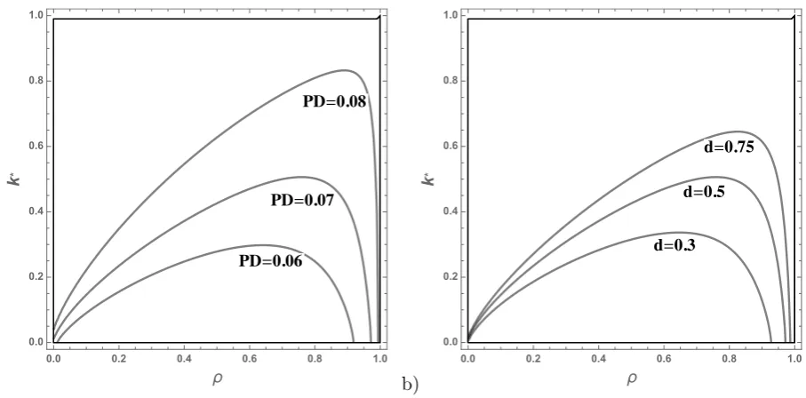
CAR dependence on the correlation
Now we focus on the case of Vasicek distribution of the loan losses (1.1), which is characterized by
two parameters — ρ and P D — the borrower’s asset correlation and the probability of borrower’s
asset default, respectively. From intuitive point of view, the larger is correlationρ, the more restrictive
banking policy is required. In other words, k∗(ρ) should be increasing function, but it is not clear,
whether the presented model catches this effect? The analytical way, like in Proposition 1, failed due
to very tedious calculations, thus, the Figures 1a and 1b show the series of computer simulations.
Figure 1a shows the curves, corresponding to the fixed discountd= 0.5and three values of the default
probabilityP D = 0.06, 0.07, 0.08. Similarly, Figure 1b shows the curves, corresponding to the fixed
probabilityP D= 0.075and three values of discountd= 0.3, 0.5, 0.75. As we see, increasing in bothd
andP D shifts the curves upwards. An interpretation of this effect is quite natural. Increasing in both
cases implies the risk of default and/or the associated losses, which forces the “responsible” banker to
be more safe and conservative. Note that Figure 1b agrees with Proposition 1 statement on ∂k∗
∂d >0.
The lack of solution in neighborhood of ρ = 0 and ρ = 1 is result of violation of the solvability
condition (2.2). The direct calculations show that for allρsufficiently close to0or1the fraction E−ˆ P D
Ret( ˆE)
exceeds d= 0.5. The values k∗ = 0, i.e., the bottom points of the “arcs”, correspond to the threshold
values ofρ, that satisfy the identity
ˆ
E −P D
Ret( ˆE;P D, ρ) =d.
The fact that “arc” of the plot starts from “bottom” point ρ1 and ends at “bottom” point ρ2, i.e.,
k∗(ρ
1) =k∗(ρ2) = 0, means that the finite solutionL∗0of the bankers’ problem exists for allρ1< ρ < ρ2. On the other hand, inequalitiesρ < ρ1andρ > ρ2imply the “bubble”L0 → ∞, which may be associated
with k∗ = 0. Therefore, we can extend the function k∗(ρ) on the “non-existence” areas ρ < ρ
1 and
a)
��=����
��=����
��=����
0.0 0.2 0.4 0.6 0.8 1.0
0.0 0.2 0.4 0.6 0.8 1.0
ρ
k
*
b)
�=���
�=���
�=����
0.0 0.2 0.4 0.6 0.8 1.0
0.0 0.2 0.4 0.6 0.8 1.0
ρ
k
[image:14.595.67.521.52.276.2]*
Figure 1: CAR k∗ as a function ofρ,R= 0.05,r = 0.15, a) d= 0.5, b) P D= 0.07
2.2 Endogenous probability of the bank’s default
The considered above optimum asset liability management is based on the risk-neutral behavior,
tar-geted to maximize the expected terminal capitalE(K1), which is nominally greater than initial capital
K0, due to Theorem 1. However, the risk of default persists even if the management decisions are
optimal. Due to (1.4) the probability of the bank’s default is equal to
p=P(ε≥ E(k∗)) = 1−F(E(k∗)),
where k∗ is solution of equation (2.4). Function 1−F(E(k)) strictly decreases with respect to k,
therefore, Proposition 1 implies that
∂p ∂d <0,
∂p ∂R <0,
∂p ∂r >0,
which is quite intuitive. Note that the equilibrium values ofk∗ must be positive, therefore, the feasible
values of the bank’s probability of default satisfy inequality p= 1−F(E(k∗))<1−F( ˆE).
Focusing on the Vasicek distribution of losses, we can consider the comparative statics of probability
pwith respect to specific parameters — the correlationρand the probability of borrower’s defaultP D.
Unfortunately, the analytic study of this question is problematic. The Figure 2 shows the result of the
computer simulations with d= 0.25,r = 0.15,R= 0.05,P D= 0.075.
Given the FOC
�
�*
=
���
�� �*>�
�*
<
�0.0 0.2 0.4 0.6 0.8 1.0
0.0 0.2 0.4 0.6 0.8 1.0
ρ
[image:15.595.59.414.230.580.2]p
we substitutek= F−1(1−p;ρ)−Eˆ
1−Eˆ obtaining the equation
H(ρ, p) =G F−
1(1−p;ρ)−Eˆ
1−Eˆ , ρ
!
= 0,
which determines the implicit function p(ρ). The set of all solutions (ρ, p) of this equation contains
the “fictive” roots, violating the feasibility condition
k∗>0 ⇐⇒ p(ρ)<1−F( ˆE, ρ).
To screen the fictive solutions we draw the delimiting border
k∗= 0 ⇐⇒ p(ρ) = 1−F( ˆE, ρ),
which is depicted by dashed curve on Figure 2. The solid curve P0P1 is a set of all feasible solution
(ρ, p), satisfying bothH(ρ, p) = 0andp(ρ)<1−F( ˆE, ρ) ⇐⇒ k∗ >0. The points(ρ, p)of the pointed
curve above the border p = 1−F( ˆE, ρ), satisfyingH(ρ, p) = 0 and p(ρ) >1−F( ˆE, ρ) ⇐⇒ k∗ <0,
are non-feasible.
As for definition of the default probability for ρ rightward to P1, let’s to recall that in these cases
the banker can not impose the self-restriction at some finite amount of the loan portfolio, which implies
L0 → ∞ ⇐⇒ k(L0)→0. Thus we may define the function k(ρ) as follows
k∗(ρ) = 0⇒p(ρ) = 1−F−1Eˆ;ρ,
i.e., the continuation of the probability of the bank default belongs to the delimiting curve p = 1−
F( ˆE, ρ).
3
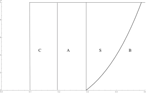
Parametric zoning by the solution types
The main aim of the present section is to visualize the various types of equilibria in terms of the model
primitives. First, assume that the deposit interest rate R, and CDF F(z) for the loan losses ε are
given and its PDF f(z) satisfies the condition ret(z) decreases for all P D < z <1. Consider the set
S of feasible points r > R, 0 ≤ d ≤ 1 of the parameter plane (r, d). With any point of this set we
associate specific type of equilibrium, which corresponds to the whole set of parameters, including the
given ones. Figure 3 shows two examples of such zoning of S for the Vasicek distribution of losses,
�
�
�
�
0.0 0.1 0.2 0.3 0.4 0.5r
0.0 0.2 0.4 0.6 0.8 1.0
[image:17.595.62.561.62.386.2]d
Figure 3: Zoning of parameters(r, d) for the Vasicek function: R= 0.1,P D= 0.04,ρ= 0.1
There are three areas in parameters space, which may be described as follows.
I. Bubble area B corresponds to the unrestricted credit expansion. It consists of points(r, d) ∈ S,
that violate condition (2.2).
II. Self-Restrained areaS corresponds to case when the bank attracts deposits and places funds to
the loan portfolio of the limited size. It consists of points (r, d)∈ S that satisfy conditions (2.2)
and ˜r > R
III. Autarchy areaAconsists of points(r, d)∈ S that satisfy the inequalityr < R˜ ,0≤d≤1, which
means that condition (2.2) trivially holds and the banker’s optimum solution is degenerate: the
bank does not attracts deposits, i.e., D0 = 0, while the the loan portfolio L0 =K0 >0.
Remark 2. For any given positive value of discount d+>0, no matter how small is it, we obtain the
nonempty intersection of the line d= d+ with all three areas. If d= 0, the Self-Constrained areaS
vanishes and we obtain only two generic cases —Bubble area B and Autarchy areaA.
The main result of this subsection is that the shapes of this zoning does not depend, on choice of
distribution function
Proof. See Appendix A.4.
3.1 The Basel III requirements
The Basel III requires that the probability of the bank’s default
p= 1−F(E(k∗))
must not exceed0.001, which implies the inequality
k∗≥¯k= VaR99.9−Eˆ 1−Eˆ .
where VaR99.9 =F−1(0.999).
The Basel III analysis uses the Vasicek loan losses distribution (1.1), therefore,
VaR99.9=F−1(0.999;P D, ρ) = Φ
r
ρ
1−ρΦ
−1(0.999) +
r
1 1−ρΦ
−1(P D)
, (3.1)
which allows to calculate the corresponding required value of CAR. Now we are going to identify sets of
the bank parametersd,r,R,P D,ρwhich guarantee that the banker complies voluntarily with Basel III
requirements, or, on the contrary, the external regulation is needed. Substituting VaR99.9 =E(¯k)into
equation (2.4), we can determine the minimum value of discount dB, as a function of r, guaranteeing
the precise discharge of Basel III requirements, as follows
dB(r) =
ˆ
E −P D
Ret(VaR99.9) + (VaR99.9−Eˆ)ret(VaR99.9)
. (3.2)
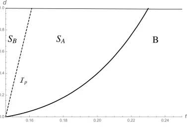
Let parameters R, P D, ρ be given, consider the curve d = dB(r) in the parameter plane (r, d).
Obviously it starts from pointd= 0,r = P D1−P D+R, moreover, function dB(r) strictly increases, because
function Eˆ = r−R
1+r is increasing with respect to r. To illustrate this division, consider the following
example withR= 0.1,P D = 0.04,ρ= 0.2, presented on Figure 4. The dashed “Basel curve” d=dB(r)
divides areaS into two sub-areas: SA, where Basel III requirements are violated, and SB, where they
are complied.
The “Basel friendly” combination of parameters admits an arbitrary value of discount d, while the
loan interest rates should not be too large. The existence of area SB may explain the paradoxical
dispersion of the observed values of CAR. Indeed, even if the values of parametersr,R,P D, andρare
the same for all bank, the dispersion of parameterdstill persists. This parameter may be idiosyncratic
�
�
�
�
�
ℐ
�0.16 0.18 0.20 0.22 0.24
r
0.0 0.2 0.4 0.6 0.8 1.0
[image:19.595.59.437.58.315.2]d
Figure 4: Dichotomy “self-restriction – external restriction”
of banker, because this parameter is applied to the decision making for the not yet defaulted bank.
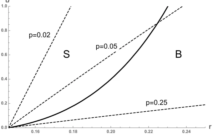
3.2 Generalized Basel and the equiprobability curves
The curve dividing areaS into two subareas in Figure 5 was determined by specific Basel III
require-ment. Let’s generalize this approach considering an arbitrary value of the bank’s default probability
pas a parameter and determining the equibrobability curve Ip associated with the value ofp, as a set
of pairs(r, d), which generate the equilibrium with the probability of default equal to p, provided that
the rest of the model parameters, including CDF F(z), are given. We also keep the assumption on
decreasing of the function ret(z)on the interval P D < z <1
Theorem 2. The assemblage of curves Ip is characterized by the following properties:
1. All curves Ipassociated with different probabilitiespstart from the same pointr= R1−+P DP D,d= 0.
2. If probability of the bank’s default pconverges to zero, then the curvesIp converge to the vertical
line r= R1−+P DP D, 0≤d≤1.
3. The assemblage of curves Ip for all p < 1−F(P D) fills the whole Self-Constrained area S,
moreover, for p < p′ the curve Ip resides leftward and above the curve Ip′.
4. For all sufficiently small p the equiprobability curve Ip does not intersect the border of the areas
B and S for 0< d≤1.
Proof. See Appendix A.5.
B
S
p=0.25 p=0.05
p=0.02
0.16 0.18 0.20 0.22 0.24 r
0.0 0.2 0.4 0.6 0.8 1.0
[image:20.595.55.396.62.280.2]d
Figure 5: Equiprobability curvesIp for p= 0.02, 0.05, 0.25.
for the Vasicek distribution of losses withP D = 0.04,ρ= 0.2, and R= 0.1. Solid curve is the border
between Self-Constrained and Bubble areas, while three dashed lines are the equiprobability curvesIp
associated with three values of the bank probability of default: for the very large probability p= 0.25
the curveIpleave the Self-Constrained area immediately, for the intermediate valuep= 0.05the curve
Ip intersect the border, while the small probability of the bank default p = 0.02 generates the curve
Ip intersecting the lined= 1.
4
Conclusion
The banking is one of the most over-regulated and over-supervised industries, and the pressure on
banks continues to grow. A natural question arises: can banks do without a regulator - at least in
some aspects of their activities that are now under strict regulation and supervision? For example,
can banks limit their credit expansion on their own, without intervention of a regulator? To answer
this question, we built a simple microeconomic model of a bank with one stochastic factor – the share
of nonperforming loans. It turns out that if the close-out sale of a loan portfolio in case of a bank
default is discountless, then the banker has no incentives to limit its credit expansion, even despite the
prospect of huge losses incurring. This means that in this case, banking cannot do without a regulator,
only the state can restrict the credit expansion.
The situation changes drastically, when we assume that in the event of a bank failure, its loan
portfolio is sold with discount. In this case, when certain limitations on the model parameters are
have learned to successfully circumvent, these restrictions are internal, and deceiving oneself is usually
not beneficial. However, from the point of view of the regulator, which evaluates the result in terms
of CAR, the level of bank self-restraint may seem inappropriate, for example, if the ratio is too low.
In this paper we derive the conditions of the existence and uniqueness of equilibrium, which have the
clear economic interpretation and appropriate for both analytical and numerical study.
It is shown that with sufficiently weak and natural restrictions on the loss distribution function,
the parameter space is divided into 3 non-empty zones in which one of the three possible outcomes
is realized: B (“Bubble”) - there are no bounded solutions (we get the outcome similar to the linear
model with zero discount); S (“Self-Constrained”) with limited solutions; and, finally, A - autarchy
solutions - deposits are not attracted, loans are placed only at own expense. In addition, a more
subtle identification of compliance with the requirements established by Basel III in the area S was
carried out. A natural dispersion of exogenous parameters, in the first place, the discount d, implies
the observed dispersion of CAR between banks.
References
[1] Astic, F., and Tourin, A. (2014), Optimal bank management under capital and liquidity
con-straints, Journal of Financial Engineering, vol. 1, no. 03, 1450022 (21 pages)
[2] Barrios, V.E., and Blanco, J.M., (2003), The effectiveness of bank capital adequacy regulation: A
theoretical and empirical approach, Journal of Banking & Finance, 27:1935–1958
[3] BIS (2019), IRB approach: risk weight functions – January
[4] BIS (2019), BIS Annual Economic Report 2019 - June
[5] Black F, Cox J.C. (1976), Valuing corporate securities: some effects of bond indenture provisions,
J. Finance, 31:351–67
[6] Black F, Scholes M. (1973), The pricing of options and corporate liabilities. J. Polit. Econ. 81:637–
54
[7] T. Bosch, J. Mukuddem-Petersen, M.P. Mulaudzi and M.A. Petersen (2008), Optimal Capital
Management in Banking, Proceedings of the World Congress on Engineering 2008 Vol II WCE
2008, July 2 - 4, London, U.K.
[8] F. Chakroun and F. Abid (2016), Capital adequacy and risk management in banking industry,
[9] DeMarzo P, Fishman M. (2007), Agency and optimal investment dynamics. Rev. Financ. Stud.
20:151–88
[10] DeMarzo P, Sannikov Y. (2006), Optimal security design and dynamic capital structure in a
continuous-time agency model. J. Finance 61:2681–724
[11] Fouche, C.H., Mukuddem-Petersen J. and Petersen M.A. (2006), Continuous-timestochastic
mod-elling of capital adequacy ratios for banks. Applied Stochastic Models in Business and Industry,
22(1):41-71.
[12] Huang, J. and M. Huang (2012), How much of the corporate-treasury yield spread is due to credit
risk?, Review of Asset Pricing Studies 2.2:153-202.
[13] Leland H. (1994), Corporate debt value, bond covenants, and optimal capital structure. J. Finance
49:1213–52
[14] Leland, H., (2004), Predictions of default probabilities in structural models of debt. Journal of
Investment Management, 2:5–20.
[15] Merton, R.C., (1974), On the pricing of corporate debt: the risk structure of interest rates. J.
Finance, 29:449–70
[16] J. Mukuddem-Petersen and M.A. Petersen (2008), Optimizing Asset and Capital Adequacy
Man-agement in Banking, J. Optim. Theory Appl. 137: 205–230
[17] Reinhart, C. M. and Rogoff, K. S. (2009) This Time Is Different: Eight Centuries of Financial
Folly, Princeton University Press
[18] Schaefer S.M, Strebulaev I. (2008), Structural models of credit risk are useful: evidence from
hedge ratios on corporate bonds. J. Financ. Econ. 90:1–19
[19] Vasicek O., (1987), Probability of Loss on Loan Portfolio, KMV Corporation
A
Appendix
Notations and abbreviations
Kt capital
Dt deposits
Mt cash
Lt loans
r loan interest rate
R deposit interest rate
ε share of nonperforming loans
(the portfolio percentage loss)
P D =E(ε) probability of default of a borrower
˜
r=r−(1 +r)P D loan risk-adjusted interest rate
d discount of loan nominal value in case of selling of the loan
k(L0) = KL00 CAR (capital adequacy ratio) – capital/risk weighted assets
ˆ E= r−R
1+r the limit threshold for the loan losses
E(k) = ˆE+ (1−Eˆ)k the threshold for the loan losses
ret(z) = (1−z)f(z) the weighted share of the returned loans
Ret(x) =R1
x ret(y)dy the expected returns of loans in case of the bank default
F(x) CDF (cumulative density function)
f(x) =F′(x) PDF (probability density function)
Φ(z) standard normal distribution
FOC First-Order Condition
SOC Second-Order Condition
ρ borrower’s asset correlation
U(L0) objective function
rf risk-free rate
A.1 Proof of Lemma
Assume first thatρ <1/2and P D≤1/2 , then in this case the PDF (1.2) is unimodal with mode at
zmode= Φ
√
1−ρ
1−2ρΦ
−1(P D)
(see, e.g., [20]). Moreover, ρ <1/2and P D≤1/2imply
√ 1−ρ
1−2ρ >1⇒
√ 1−ρ
1−2ρΦ
−1(P D)
≤Φ−1(P D)⇒zmode≤Φ(Φ−1(P D)) =P D,
becauseΦ−1(P D)≤0, therefore,f(z) decreases with respect toz, as well as (1−z)f(z) does.
Now assume that 1 > ρ≥1/2 and P D ≤1/2. Substituting x = Φ−1(z) we obtain the following
problem: to prove that the function
h(x) =
r
1−ρ ρ exp
1 2
"
x2−
√
1−ρx−c
√ρ
2#!
(1−Φ(x)) =ϕ
√
1−ρx−c
√ρ
Φ(−x)
ϕ(x)
is decreasing with respect to x, where c = Φ−1(P D) < 0, ϕ(z) = Φ′(z) > 0 is the density function
of the standard normal distribution satisfying the identity ϕ′(x) = −xϕ(x). Differentiating h(x) we
obtain
h′(x) =
ϕ√1−√ρxρ−c
ϕ(x)
c√1−ρ ρ +
2ρ−1
ρ x
Φ(−x)−ϕ(x)
.
Assume first thatx≤0. Given c= Φ−1(P D)≤0, we obtain
c√1−ρ ρ +
2ρ−1
ρ x
Φ(−x)−ϕ(x)<0⇒h′(x)<0.
Now let x >0, then
c√1−ρ ρ +
2ρ−1
ρ x
Φ(−x)−ϕ(x)< xΦ(−x)−ϕ(x)<0,
due to
2ρ−1
ρ = 1−
1−ρ ρ <1
and ϕ(x)> xΦ(−x) for allx≥0. Indeed,ϕ(0)>0 = 0·Φ(−0)and for allx >0 the inequality
ϕ′(x) =−xϕ(x) =−xϕ(−x)>Φ(−x)−xϕ(−x) = (xΦ(−x))′
holds, which completes the proof of this case.
Finally, assume that P D >1/2, thenc= Φ−1(P D)>0, and z > P Dimplies x= Φ−1(z)> c >0
and, consequently,
c√1−ρ ρ +
2ρ−1
ρ x <
2ρ−1 +√1−ρ
ρ x=x−
√
1−ρ(1−√1−ρ)
for all 0< ρ <1. The rest of proof is similar. Q.E.D.
A.2 Proof of Theorem 1
Proof. Differentiating the function (2.1), we obtain
U′(L0) = ˆE −P D−d·
Ret(E(k(L0))) + (1−Eˆ)k(L0)ret(E(k(L0))
(A.1)
while the second derivative takes on the form
U′′(L0) =−d·
−ret(E(k(L0))dE dL0
+ (1−Eˆ)ret(E(k(L0)) dk dL0
+ (1−Eˆ)k(L0)ret′(E(k(L0))dE dL0
=
= d
L0 ·
(1−Eˆ)2k2(L0)ret′(E(k(L0))<0, (A.2)
due to
dE dL0
= (1−Eˆ) dk
dL0
= (1−Eˆ)k(L0)
L0
.
To justify the solvability of equation U′(L
0) = 0 on the interval (K0,+∞), note that
U′(K0) = ˆE −P D−d(1−F(1)−P D+Ret(0)) = ˆE −P D >0,
while for all sufficiently large L0 the values ofU′(L0) are negative under the conditions of Theorem.
Indeed,
lim
L0→∞
U′(L0) = ˆE −P D−d·Ret( ˆE)<0 ⇐⇒ d >
ˆ
E −P D
Ret( ˆE) .
Given the SOC U′′<0, we obtain that there exists the unique solution of the FOCU′(L
0) = 0. Due
to (A.1) we may represent the FOC as the equation
ˆ
E −P D−d·Ret(E(k)) +1−Eˆk·ret(E(k))= 0
of variable k = K0/L0, which sets the correspondence between solution of this equation k∗ and the
equilibrium size of the loan portfolio L∗
0.
A.3 Proof of Proposition 1
To simplify calculations, consider the following substitution of variables E = ˆE+ (1−Eˆ)k. Then the
FOC (2.4) is equivalent to the equation
G(E)≡E −ˆ P D−d·Ret(E) +E−Eˆret(E)= 0.
Let E∗ be the solution of this equation, considered as an implicit function of all parameters. The
corresponding derivative with respect to an arbitrary parameterais as follows
∂E∗
∂a =− ∂G
∂a
∂G
∂E,
where
∂G ∂E =d·
E−Eˆ(f(E)−(1−E)f′(E)) =−d·E−Eˆret′(E)>0,
becauseE >Eˆand ret(E)is a decreasing function. Moreover,
∂G ∂d =−
Ret(E) +E−Eˆret(E)<0,
which implies ∂E∂d∗ >0.
Now let a=R, given
ˆ
E= r−R
1 +r
we obtain
∂G ∂R =−
1
1 +r −d·
ret(E) 1 +r <0,
which implies ∂E∂R∗ >0. Furthermore, the inequality
∂G ∂r =
1 +R
(1 +r)2 +d·
(1 +R)ret(E) (1 +r)2 >0
implies ∂E∂r∗ <0.
Given E∗= (1−Eˆ)k∗+ ˆE and Eˆ= r−R
1+r, we obtain that
k∗ = (1 +r)E∗−(r−R)
1 +R , L
∗
0 =
(1 +R)K0
(1 +r)E∗−(r−R), D∗0 =L∗0−K0,
therefore,
∂k∗
∂d >0, ∂L∗
0
∂d <0, ∂D∗
0
Moreover,
∂k∗
∂R =−
1 +r
(1 +R)2E∗+
1 +r
1 +R ∂E∗
∂R +
1 +r
(1 +R)2 =
1 +r
(1 +R)2(1−E∗) +
1 +r
1 +R ∂E∗
∂R >0,
∂L∗0 ∂R =
∂D∗0 ∂R =
K0((1 +r)E∗−(r−R))−(1 +R)K0 (1 +r)∂E ∗
∂R + 1
((1 +r)E∗−(r−R))2 =
=−(1 +r)K0 (1−E
∗) + (1 +R)∂E∗
∂R
((1 +r)E∗−(r−R))2 <0,
becauseE∗ <1 , ∂E∂R∗ >0.
Finally,
∂k∗
∂r =
1 1 +R
(1 +r)∂E∗
∂r −(1−E
∗) <0 ∂L∗ 0 ∂r = ∂D∗ 0
∂r =−
(1 +R)K0
((1 +r)E∗−(r−R))2
E∗−1 + (1 +r)∂E∗
∂r
>0,
because of E∗<1and ∂E∗
∂r <0. Q.E.D.
A.4 Proof of Proposition 2
The statement about area A is obvious. The rest is to show the robustness of shapes of areas B and
S. Note that the function
dS(r) =
ˆ
E(r)−P D
Ret( ˆE(r)) ,
whereEˆ(r) = r1+−Rr, satisfies the following conditions:
1. dS
P D+R
1−P D
= 0,
2. dS(r)strictly increases for allr > P D1−P D+R.
The first statement is obvious due to definition of dS(r). Then, representing the function dN(r) as
follows
dS(r) =
˜
r−R
1 +r ·
1
Retr1+−Rr
,
and given the functions r˜−R
1+r, r−R
1+r are positive and strictly increasing with respect tor we obtain that
the function d0(r) is also strictly increasing. Finally, the function dS(r) is unrestrictedly increasing
withr→ ∞, because
˜
r−R
1 +r →1−P D,
r−R
1 +r →1.
the curvilinear triangle S. Q.E.D.
A.5 Proof of Theorem 2
Consider the probability of the bank’s defaultp as a parameter with possible values from the interval
[0,1]. Formula (1.4) implies that for any given p, the equation p = 1−F(E) determines the value
Ep =F−1(1−p). This means that the equiprobability curve Ip is determined by equation
ˆ
E(r)−P D−d·Ret(Ep) +
Ep−Eˆ(r)
ret(Ep)
= 0,
or, equivalently,
d=dp(r)≡
ˆ
E(r)−P D
Ret(Ep) +
Ep−Eˆ(r)
ret(Ep)
, (A.3)
whereEˆ(r) = r1+−Rr. It is obvious thatdp
P D+R
1−P D
= 0for all p, which completes the first statement of
the theorem. Moreover, p → 0 implies Ep → 1, therefore, lim
p→0dp(r) = +∞ for any r >
R+P D
1−P D ⇐⇒
ˆ
E(r)−P D >0, which completes the second statement.
Recall that the border of areas S andB is determined by the function
dS(r) =
ˆ
E(r)−P D
Ret( ˆE(r)) .
Calculating and comparing the derivatives of dS(r) and dp(r) at the starting pointr0 = R1−+P DP D
d
drdS(r0) =
(1−P D)2 (1 +R)Ret(P D),
d
drdp(r0) =
(1−P D)2
(1 +R) (Ret(Ep) + (Ep−P D)ret(Ep))
,
we obtain that
d
drdp(r0)>
d
drdS(r0) ⇐⇒ Ret(P D)>Ret(Ep) + (Ep−P D)ret(Ep).
Consider the function
G(x) =Ret(x) + (x−P D)ret(x),
which obviously satisfiesG(P D) =Ret(P D). Moreover,
for all x > P D. This implies that
x=Ep =F−1(1−p)> P D ⇐⇒ p <1−F(P D)
is necessary and sufficient condition for the curveIpto belong the areaS, at least in some neighborhood
of r0.
Let’s determine the point of intersection of the equiprobability curveIp with the border of areasS
and Bfrom the following equation
dS(r) =dP(r) ⇐⇒ Ret( ˆE(r)) =Ret(Ep) +
Ep−Eˆ(r)
ret(Ep).
The unique solution r(p) of this equation is determined by identity
Ep = ˆE(r(p)) ⇐⇒ r(p) =
Ep+R
1−Ep
= F−
1(1−p) +R
1−F−1(1−p) > r0 =
P D+R
1−P D
becauseF−1(1−p)> P D. Note that this point of intersection is actual only in case
dS(r(p)) =dp(r(p))≤1,
otherwise, the equiprobability curve intersects the line d = 1 instead of dS(r). This happens if and
only if
dS(r(p))>1 ⇐⇒ Ep−P D−Ret(Ep)>0.
Note that the function
H(x) =x−P D−Ret(x)
for x ≥ P D satisfies the following conditions: H(P D) < 0, H(1) = 1−P D > 0, and H′(x) =
1 + (1−x)f(x) > 0. This implies that there is x∗ ∈ (P D,1) such that for all x > x∗ the function
H(x)>0, which is equivalent to
p <1−F(x∗)⇒Ep−P D−Ret(Ep)>0.