Proceedings of the 55th Annual Meeting of the Association for Computational Linguistics (Short Papers), pages 484–490 Vancouver, Canada, July 30 - August 4, 2017. c2017 Association for Computational Linguistics
Proceedings of the 55th Annual Meeting of the Association for Computational Linguistics (Short Papers), pages 484–490 Vancouver, Canada, July 30 - August 4, 2017. c2017 Association for Computational Linguistics
A Network Framework for Noisy Label Aggregation in Social Media
Xueying Zhan1, Yaowei Wang1, Yanghui Rao1,∗, Haoran Xie2, Qing Li3, Fu Lee Wang4, Tak-Lam Wong2
1School of Data and Computer Science, Sun Yat-sen University, Guangzhou, China
2Department of Mathematics and Information Technology, The Education University of Hong Kong, Hong Kong SAR
3 Department of Computer Science, City University of Hong Kong, Hong Kong SAR
4 Caritas Institute of Higher Education, Hong Kong SAR
{zhanxy5, wangyw7}@mail2.sysu.edu.cn, [email protected], [email protected], [email protected], [email protected], [email protected]
Abstract
This paper focuses on the task of noisy label aggregation in social media, where users with different social or culture back-grounds may annotate invalid or malicious tags for documents. To aggregate noisy la-bels at a small cost, a network framework is proposed by calculating the matching degree of a document’s topics and the annotators’ meta-data. Unlike using the back-propagation algorithm, a probabilis-tic inference approach is adopted to esti-mate network parameters. Finally, a new simulation method is designed for vali-dating the effectiveness of the proposed framework in aggregating noisy labels.
1 Introduction
Social media allows users to share their views, opinions, emotion tendencies, and other person-al information online. It is quite vperson-aluable to ana-lyze and predict user opinions from these materials (Wang and Pal,2015), in which supervised learn-ing is one of the effective paradigms (Xu et al.,
2015). However, the performance of a supervised learning algorithm relies heavily on the quality of training labels (Song et al.,2015). In social media, many training data are collected via simple heuris-tic rules or online crowdsourcing systems, such as Amazon’s Mechanical Turk (www.mturk.com) which allows multiple labelers to annotate the same object (Zhang et al.,2013). Due to the lack
∗The corresponding author.
of quality control, it can be hard for a model to reconcile such noise in training labels.
This study aims to aggregate noisy labels by matching annotators and documents. Unlike other noisy label aggregation and integration tasks (or algorithms), such as Learning to Rank (LtR) and integrating crowdsourced labels which rely on ac-curate instance sources (Ustinovskiy et al., 2016) or confidence scores (Oyama et al.,2013), we on-ly need features that can be obtained with a small cost (i.e., topics). Compared with acquiring accu-rate instance sources or confidence scores, which is very hard, extracting topics can be done con-veniently by many existing topic models. Note that label noise is not always random, as adver-sarial noisemay occur in real-world environments when a malicious agent is permitted to select la-bels for certain instances (Auer and Cesa-Bianchi,
1998). For example, a fake annotator is purchased to promote defective goods by giving high ratings. Noisy labels in such a manner are extremely dif-ficult to be handled (Nicholson et al., 2015). To validate the effectiveness of aggregating the afore-mentioned noisy labels, we propose to design a new simulation method in Section4.
2 Related Work
To aggregate or refine noisy labels, several ap-proaches have been proposed recently. Whitehill et al. (Whitehill et al., 2009) explored a proba-bilistic model to combine labels from both human labelers and automatic classifiers in image classi-fication. Raykar et al. (Raykar et al., 2010) used a Bayesian approach for supervised learning over
noisy labels from multiple annotators. Oyama et al. (Oyama et al.,2013) proposed to integrate la-bels of crowdsourcing workers using their con-fidence scores. Song et al. (Song et al., 2015) developed a single-label refinement algorithm to adjust noisy and missing labels. Ustinovskiy et al. (Ustinovskiy et al., 2016) proposed an opti-mization framework via remapping and reweight-ing methods to solve the problem of LtR with the existence of noisy labels.
Different from the previous study that modeled the difficulties of instances and the user’s author-ity (Whitehill et al., 2009), we target at integrat-ing multiple labels for each instance by estimat-ing the matching degreeof documents and anno-tators. Consequently, our work is applicable to aggregating individual sentiment labels in social media, where users under various scenarios (e.g., character and preference) may express invalid or noisy sentiments to different topics.
3 Noisy Label Aggregation Framework
3.1 Problem Definition
The problem of noisy label aggregation is defined as follows: GivenN documents (instances) anno-tated byM users (annotators) overC kinds of la-bels, we generate D topics by existing unsuper-vised topic models. LetT ∈ RN×D be topics of all instances, where thei-th row ofT(i.e.,Ti) is the topic distribution of documenti, and the size ofTi(i.e.,|Ti|) isD. LetF∈RM×Ube features (e.g., age and gender) of all annotators, whereFj is the feature distribution of userjand|Fj|=U. To model different dimensions of document topics (D) and annotator features (U) jointly, we mapTi andFj toK latent factors denoted asSi andAj, i.e.,|Si|=|Aj|=K.
words f topics i Ζ 1 A 2 A j A 1 i V 2 i
V Vij
i S iC Z w ei gh t la b el s o n e-m ax p o o li n g to p ic ex tr ac tio n fu lly -co n n ec te d m at ch in g d eg re e
[image:2.595.81.278.600.724.2]weight transformation with softmax
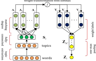
Figure 1: Our proposed network framework.
To estimate the ground truth labelZi, we pro-pose a novel network framework via aggregating the observable labelsVi, as shown in Fig. 1. In
our framework, the correctness ofVij depends on whether annotatorjmatchesdocumenti.
3.2 Detailed Steps
Topic Extraction (TE): For document features, it is rough to use tf ortf-idf since they ignore the versatility of semantics among various contexts. Without considering the semantic units called top-ics, the accurate category of each document may be hard to access (Song et al.,2016). Short mes-sages (e.g., tweets) are prevalent in social media, which differ from normal documents insofar as the number of words is fewer and most words only oc-cur once in each instance. To extract topics from such a sparse word space, we employ the Biterm Topic Model (BTM) by breaking each document into biterms and leveraging the information of the whole corpus (Yan et al.,2013).
Fully-connected Operation (FcO): There can be a large difference between dimensions of doc-ument topics and annotator features, so we need convert T and F to the same latent space. This
step conducts linear transformation by introduc-ing fully-connected weights WT ∈ RD×K and
WF ∈ RU×K, as follows: S = TWT and
A = FWF. The values of SandAare
propor-tional to the label correctness probability.
Since more cohesive topics may indicate that the document’s category is more concentrated and can be correctly annotated by more users, the topic distribution embeds key information on the document factors S. To map T to S well, we
propose the concept of topic entropy that acts as the constraint factor, by calculating the cen-tralization of each document’s topics: H(di) =
−∑Dz=1p(tz|di) logD
(
p(tz|di) )
, where p(tz|di) is the probability of thez-th topic conditioned to documenti, and D constrains the values ranging from0to1. The lowerH(di), the higher the con-centration of topics and the label correctness for document i. We thus infer the relationship be-tweenSi andH(di)as||Si||2 ∝1/H(di), where
||Si||2is the Euclidean norm ofSi.
Matching Degree Calculation (MDC): This step calculates the matching degreeof document iand annotatorj, which is denoted asgij by the similarity/distance between latent factors Si and
close to a document i that contains the “basket-ball” topic, which indicates that the “matching de-gree” ofiandjis high with a large similarity. The inner product is used here, and it can be replaced by distance measures.
Weight Transformation (WT): We employ transformation to distinguish different scores ef-fectively. The activation function issigmoid (soft-max) ortanh. Since most document labels are as-sumed to be discrete independent variables, we en-code Vij as a binary vector. The higher gij of a label, the closer it is to the ground truth. Namely, we should weight these labels in such a way that if a label has highgij, its weight will be increased; meanwhile, other labels should be punished. For sigmoidandtanh, the punishment is1−wij and
−wij, respectively. Take four labels, the transfor-mation weightwij andVij = (1,0,0,0)as an ex-ample, the label weight via sigmoid is Vnew
ij =
(wij,1−wij,1−wij,1−wij).
Label Weighting (LW) and One-max Pooling: The final step is to output by integrating weight-ed labels, where the multiplicative combination is used in aggregation, and the output is the maxi-mum one of aggregated labelsZiC.
3.3 Parameter Estimation
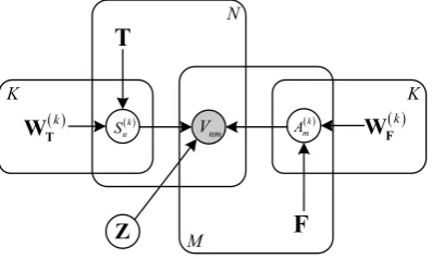
Since training labels may contain noise, it is in-accurate to employ the back-propagation method which uses the error between predicted and train-ing labels as feedback for parameter estimation. Thus, we turn the estimation of model parameters
WT and WF into a probabilistic problem. The
graphical representation is illustrated in Fig.2.
K
nm V
M N
K
( )k T
W ( )k
n
S ( )k
F W ( )k m
A T
[image:3.595.83.282.539.658.2]F Z
Figure 2: Probabilistic graphical representation.
Firstly, we define W = {WT,WF} for
sim-plicity. Secondly, the parameter distribution is de-termined by the Maximum A Posteriori (MAP) principal: W∗ = arg maxWP r(W|V,T,F) = arg maxW∑ZP r(Z)P r(W|V,T,F,Z).
Finally, the following Expectation Maximiza-tion (EM) algorithm is used to estimateW∗.
Initialization: We first initializeW randomly. The prior of ground truthZcan be set to1/C or the frequency of each observable label.
Expectation (E): We then compute the expecta-tion of the joint log-likelihood of observable and hidden variables given W (i.e., the Qfunction), as follows: Q(W) =E[lnP r(V,Z,T,F|W)] =
E[lnP r(V|Z,T,F,W)]+E[lnP r(Z,T,F|W)].
Maximization (M): According to the Q func-tion, the maximum likelihood of hidden variables is estimated by the gradient ascent method.
Alternation: The above E and M steps are alter-nately performed until the likelihood converges.
4 Experiments
4.1 Datasets and Baselines
As sentiment and emotion detection are widely studied in social media analysis (Wang and Pal,
2015), we test model performance based on the Stanford Twitter Sentiment (STS) and the Interna-tional Survey on Emotion Antecedents and Reac-tions (ISEAR) corpus. The original STS dataset (Go et al., 2009) contains1.6 million tweets that
were automatically labeled as positive or negative using emoticons as labels, in which 80K (5%)
randomly selected tweets were used to speed up the training process, 16K (1%) randomly
select-ed tweets were usselect-ed as the validation set, and
359 tweets were manually annotated as the
test-ing set (dos Santos and Gatti, 2014). ISEAR is composed of7,666sentences annotated by1,096
participants with different culture backgrounds (Scherer and Wallbott, 1994). These participants completed questionnaires about their 34 kinds of
personal information (e.g., age, gender, city, coun-try, and religion), as well as their experiences and reactions over seven emotions. For the ISEAR corpus, we randomly selected 60% of sentences
as the training set,20%as the validation set, and the remaining20%as the testing set.
We use the following models for comparison: Majority Voting (MV) (Sheng et al.,2008), Maxi-mum Likelihood Estimator (MLE) (Raykar et al.,
2010), and Generative model of Labels, Abilities and Difficulties (GLAD) (Whitehill et al., 2009). The baselines of MV and MLE are implement-ed by following (Sheng et al.,2008;Raykar et al.,
also implement the multivariate version of GLAD, called MGLAD as the baseline for the ISEAR corpus with seven emotions. Although there are some more recent models on label aggregation (Oyama et al., 2013) or refinement (Song et al.,
2015;Ustinovskiy et al.,2016), they either require additional features like users’ reported confidence scores, or are only suitable to a corpus with one label for each document. To compare sentiment and emotion classification performance using the aggregated labels for training, we further apply the above noisy label aggregation models to a lin-ear Support Vector Machine (SVM) with squared hinge loss (Chang and Lin, 2011). As shown in the existing studies with refined labels, the lin-ear SVM performed well on sentiment classifi-cation of reviews (Pang et al., 2002) and tweets (Vo and Zhang,2015).
4.2 Experimental Design
To evaluate the performance of noisy label ag-gregation models, each instance should be anno-tated by multiple users. Unlike previous studies which introduced a parameter to disturb ground truth labels (Sheng et al., 2008) or employed online crowdsourcing systems (Whitehill et al.,
2009; Raykar et al., 2010) to generate noisy an-notations, we design a new simulation approach by following the process of Profile Injection Attack in Collaborative Recommender Systems (Williams and Mobasher, 2006). This is because the existing methods can not assign multiple labels to each instance, or are difficult to generate virtual users and access their information (e.g., age and gender). In particular, the following steps have been performed. First, we generate virtual user-s with different featureuser-s, making them the neigh-bors of existing (actual) annotators. For each di-mension of the actual annotators’ features, we take the mean value if the attribute is continuous. For discrete attributes, we randomly select one type from the existing attribute values. If the dataset has no user features, we set it as a unit vector. Second, we generate document annotating vectors for virtual users. Each annotating vector is com-posed of three parts: annotating for filler instances (IF), which is a set of randomly chosen filler in-stances drawn from the whole dataset, untagged instances (I∅), and the target instance (it). The
purpose of settingIF andI∅ is to make the
vir-tual user looks like an ordinary annotator. We
select three simulation types from Profile Injec-tion Attack (Williams and Mobasher,2006), i.e., random, average, and love/hate. In the random method, the label for each instance i ∈ IF is drawn from a normal distribution around the an-notations across the whole dataset, and the prob-ability of labeling correctly toiis1/C. The
cor-responding probabilities are0.5 and1 for the
av-erage and love/hate methods, respectively. In all these methods, the annotation for it is randomly selected from wrong labels.
We tune the number of topics D and annota-tor features U by performing a grid search over all D and U values, with D ∈ {2,3,4, ...,10}
on both datasets, U = 34 on ISEAR, and U ∈
{1,10,100,500,1000}on STS that contains user ID only. The value ofK is set to the maximum of DandU. Based on the performance on the vali-dation set, we setD = 6, U = 1000, K = 1000
for STS, andD= 2, U = 34, K = 34for ISEAR.
For the sum of|IF|and|it|(i.e., attack size) for each virtual user, we set it as the mean number of annotations in actual users. The sum of se-lectingit in each simulation is called the profile size, and the percentage of the profile size is de-noted as o. Following the previous criterion of choosing the noise rate (Auer and Cesa-Bianchi,
1998), we set o ∈ {0.05, 0.1, 0.2, 0.5}. Ac-cording to (Ustinovskiy et al., 2016), each target instance except for those in IF is annotated by three users. Thus, the number of virtual users is set to 2oN. We set the parameter values of MV, MLE, and M/GLAD according to (Sheng et al.,
2008;Raykar et al.,2010;Whitehill et al.,2009), and apply the grid search method to obtain the op-timal parameters for SVM.
4.3 Results and Analysis
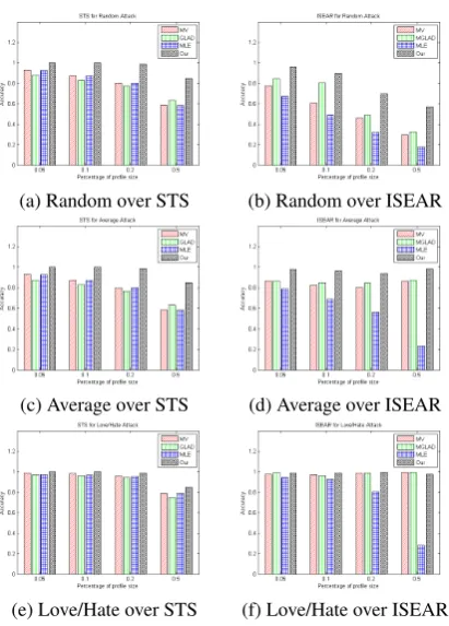
Firstly, we evaluate the noisy label aggregation performance of different models by comparing the proportion of estimated labels which match the ac-tual categories (i.e., accuracy). The results are shown in Fig. 3, which indicates that our model performs the best under various conditions. From the aspect of simulation methods, the accuracy of the random one is the lowest and the Love/Hate one is the highest, which is consistent to the cor-rectly labeling probability for each method. The results of the random and average ones over STS are similar, becauseC= 2on STS.
(a) Random over STS (b) Random over ISEAR
(c) Average over STS (d) Average over ISEAR
[image:5.595.78.284.59.346.2](e) Love/Hate over STS (f) Love/Hate over ISEAR Figure 3: Label aggregation performance.
baselines in aggregating noisy labels, especially when the noise scale becomes large. For instance, our model achieves 85% and57% accuracies on
STS and ISEAR when using the random method ando = 0.5, which indicates that our model has higher capability of recognizing adversarial noise (it). In the random method, we can also observe that the performance differences are more signifi-cant on ISEAR than STS. This is because ISEAR has more elaborate, i.e., 34 kinds of observable
user information, which validates the joint influ-ence of users and documents on noisy label aggre-gation. To evaluate the performance differences statistically, we use the12 groups of results over all methods andovalues based on the convention-al significance level (i.e., p value) of 0.05. The
p values of t-tests between our model and MV, M/GLAD, MLE are0.0087,0.0009,0.0067over
STS, and 0.0535, 0.1037, 0.0007 over ISEAR,
which indicates that the performance differences between our model and baselines are statistically significant on both datasets, except for MV and MGLAD in the love/hate method over ISEAR. The reason may be that each virtual user annotates around seven instances on ISEAR, and only one label is incorrect for the love/hate method, which makes the simple MV perform competitively.
Secondly, we compare the classification
perfor-(a) Random over STS (b) Random over ISEAR
(c) Average over STS (d) Average over ISEAR
[image:5.595.313.517.60.347.2](e) Love/Hate over STS (f) Love/Hate over ISEAR Figure 4: Classification performance.
mance of SVM using labels from different noisy label aggregation models for training. The accura-cies are shown in Fig.4, in which dotted lines rep-resent results on benchmark datasets without con-ducting the Profile Injection Attack process. Com-pared to other methods, the performance of SVM based on the aggregated labels from our model is almost closer to that of SVM using benchmark datasets. For the average method and o = 0.2
over STS, we can observe that SVM in conjunc-tion with our model performs even better than that on the benchmark dataset. This is because emoti-cons are used as annotations for STS, which may introduce errors to the original labels.
5 Conclusions
Acknowledgments
The authors are thankful to the reviewers for their constructive comments and suggestions on this pa-per. The work described in this paper was support-ed by the National Natural Science Foundation of China (61502545), a grant from the Research Grants Council of the Hong Kong Special Admin-istrative Region, China (UGC/FDS11/E03/16), the Start-Up Research Grant (RG 37/2016-2017R), and the Internal Research Grant (RG 66/2016-2017) of The Education University of Hong Kong.
References
P. Auer and N. Cesa-Bianchi. 1998. On-line learning with malicious noise and the closure algorithm. An-nals of Mathematics and Artificial Intelligence 23(1-2):83–99.
C.-C. Chang and C.-J. Lin. 2011. LIBSVM: A li-brary for support vector machines. Journal of ACM Transactions on Intelligent Systems and Technology 2(3):27:1–27:27.
C.N. dos Santos and M. Gatti. 2014. Deep convo-lutional neural networks for sentiment analysis of short texts. InProceedings of the 25th Internation-al Conference on ComputationInternation-al Linguistics (COL-ING). pages 69–78.
A. Go, R. Bhayani, and L. Huang. 2009. Twitter sen-timent classification using distant supervision. C-s224n Project Report.
B. Nicholson, J. Zhang, V.S. Sheng, and Z. Wang. 2015. Label noise correction methods. In IEEE International Conference on Data Science and Ad-vanced Analytics (DSAA). pages 1–9.
S. Oyama, Y. Baba, Y. Sakurai, and H. Kashima. 2013. Accurate integration of crowdsourced labels using workers’ self-reported confidence scores. In Pro-ceedings of the 23rd International Joint Conference on Artificial Intelligence (IJCAI). pages 2554–2560.
B. Pang, L. Lee, and S. Vaithyanathan. 2002. Thumb-s up? Thumb-sentiment claThumb-sThumb-sification uThumb-sing machine learn-ing techniques. InProceedings of the Conference on Empirical Methods in Natural Language Processing (EMNLP). pages 79–86.
V.C. Raykar, S. Yu, L.H. Zhao, G.H. Valadez, C. Florin, L. Bogoni, and L. Moy. 2010. Learning from crowd-s. Journal of Machine Learning Research11:1297– 1322.
K.R. Scherer and H.G. Wallbott. 1994. Evidence for universality and cultural variation of differential e-motion response patterning. Journal of Personality & Social Psychology66(2):310–328.
V.S. Sheng, F. Provost, and P.G. Ipeirotis. 2008. Get another lable? improving data quality and data min-ing usmin-ing multiple, noisy labelers. InProceedings of the 14th ACM SIGKDD International Conference on Knowledge Discovery and Data Mining (SIGKDD). pages 614–622.
K. Song, W. Gao, L. Chen, S. Feng, D. Wang, and C. Zhang. 2016. Build emotion lexicon from the mood of crowd via topic-assisted joint non-negative matrix factorization. In Proceedings of the 39th International ACM SIGIR conference on Research and Development in Information Retrieval (SIGIR). pages 773–776.
Y. Song, C. Wang, M. Zhang, H. Sun, and Q. Yang. 2015. Spectral label refinement for noisy and miss-ing text labels. In Proceedings of the 29th AAAI Conference on Artificial Intelligence (AAAI). pages 2972–2978.
Y. Ustinovskiy, V. Fedorova, G. Gusev, and P. Serdyukov. 2016. An optimization framework for remapping and reweighting noisy relevance labels. In Proceedings of the 39th International ACM SIGIR Conference on Research and Development in Information Retrieval (SIGIR). pages 105–114. D. Vo and Y. Zhang. 2015. Target-dependent
twit-ter sentiment classification with rich automatic fea-tures. InProceedings of the 24th International Joint Conference on Artificial Intelligence (IJCAI). pages 1347–1353.
Y. Wang and A. Pal. 2015. Detecting emotions in so-cial media: A constrained optimization approach. In Proceedings of the 24th International Joint Confer-ence on Artificial IntelligConfer-ence (IJCAI). pages 996– 1002.
J. Whitehill, P. Ruvolo, T. Wu, J. Bergsma, and J.R. Movellan. 2009. Whose vote should count more: Optimal integration of labels from labelers of un-known expertise. InProceedings of the 23rd Annual Conference on Neural Information Processing Sys-tems (NIPS). pages 2035–2043.
C.A. Williams and B. Mobasher. 2006. Thesis: Profile injection attack detection for securing collaborative recommender systems. Service Oriented Computing & Applications1(3):157–170.
R. Xu, T. Chen, Y. Xia, Q. Lu, B. Liu, and X. Wang. 2015. Word embedding composition for data imbal-ances in sentiment and emotion classification. Cog-nitive Computation7(2):226–240.
X. Yan, J. Guo, Y. Lan, and X. Cheng. 2013. A biterm topic model for short texts. In Proceedings of the 22nd International Conference on World Wide Web (WWW). pages 1445–1456.
A ISEAR’s Annotator Features
The ISEAR corpus contains 34 kinds of personal information of participants. For clarity, the total set of annotator features is given below.
• Subject’s backgrounds: (1) city, (2) Country,
(3) ID suffix, (4) gender, (5) age, (6)
reli-gion, (7) practising religion, (8) father’s job,
(9) mother’s job, and (10) field of study.
• Questionnaire: (11) when did the situation or
event happen? (12) how long did you feel the
emotion? (13) how intense was this feeling?
• Physiological symptoms of participants: (14)
ergotropic arousal, (15) trophotropic arousal,
and (16) felt temperature.
• Expressive behavior and other features of participants: (17) movement behavior, (18)
laughing or smiling, (19) crying or sobbing,
(20) nonverbal activity, (21) paralinguistic
activity, (22) verbal activity, (23) moving
a-gainst people or things, aggression, (24) did
you expect the situation or event that caused your emotion to occur? (25) did you try to
hide or to control your feelings so that no-body would know how you really felt? (26) did you find the event itself pleasant or un-pleasant? (27) would you say that the
situ-ation or event that caused your emotion was unjust or unfair? (28) did the event help or
hinder you to follow your plans or to achieve your aims? (29) who do you think was re-sponsible for the event in the first place? (30)
how did you evaluate your ability to act on or to cope with the event and its consequences when you were first confronted with this sit-uation? (31) if the event was caused by your
own or someone else’s behavior, would this behavior itself be judged as improper or im-moral by your acquaintances? (32) how did
this event affect your feelings about yourself, such as your self-esteem or your self confi-dence? (33) how did this event change your
relationships with the people involved? and (34) the “NEUTRO” attribute.
B Noisy Label Aggregation Algorithm In our method of noisy label aggregation as shown in Algorithm 1, the cost of calculating S
andAbyFcO (line 6) is linear to the number of
Algorithm 1Noisy Label Aggregation
Input:
V: Observable labels; F: Features of users;
ω: Words of documents; δ: Threshold of convergence.
Output:
Aggregated labels. 1: T←TE(ω);
2: Initialize parameterWrandomly;
3: Q←0; 4: repeat
5: lastQ←Q;
6: {S,A} ←FcO(W,T,F); 7: foreachi∈[1, N]do
8: foreachj∈[1, M]do
9: gij =M DC(Si,Aj);
10: Vijnew=W T(gij, Vij, sigmoid);
11: end for
12: ZiC =LW(Vnewi ); 13: end for
14: Q←E-Step(ZiC); 15: W←M-Step(Q,W);
16: until|Q-lastQ|< δ;
17: return Zi,i.e., the maximum one ofZiC.
instances, i.e., O(N DK), and the total number
of users,i.e.,O(M U K), respectively. Before the
EM iteration (lines 7 to 13), it takesO(N M(K+
C))to weigh all labels V. For each iteration of
EM (lines 14 to 15), the optimization with stochas-tic gradient descent takesO(N M C+N K+M K)
when each user annotates all documents. Assume that our algorithm converges aftertiterations (t <
10in our experiments), the overall time
complex-ity is O(N M(K +C)t), which is linear to the
numbers of instances and users.
C Gradient Derivation
Given the estimated value ofZiC, theQfunction can be calculated byQ(W) =∑ijZiClnVijnew+ const. Since the vector Vijnew has two possible values when using sigmoid (i.e., wij and 1 − wij), the gradient of lnVijnew on parameter W
i,k T is(Vij−wij)Ajk,i.e.,[wij(1−wij)]/wijAjk and