A new method for Quantitative Trait Loci Detection

A new method for Quantitative Trait Loci Detection

Charles-Elie Rabier, C´

eline Delmas

To cite this version:

Charles-Elie Rabier, C´

eline Delmas. A new method for Quantitative Trait Loci Detection.

2010.

<

hal-00610615

>

HAL Id: hal-00610615

https://hal.archives-ouvertes.fr/hal-00610615

Submitted on 23 Jul 2011

HAL

is a multi-disciplinary open access

archive for the deposit and dissemination of

sci-entific research documents, whether they are

pub-lished or not.

The documents may come from

teaching and research institutions in France or

abroad, or from public or private research centers.

L’archive ouverte pluridisciplinaire

HAL

, est

destin´

ee au d´

epˆ

ot et `

a la diffusion de documents

scientifiques de niveau recherche, publi´

es ou non,

´

emanant des ´

etablissements d’enseignement et de

recherche fran¸

cais ou ´

etrangers, des laboratoires

publics ou priv´

es.

A new method for Quantitative Trait Loci detection

Charles-Elie Rabier

Institut de Mathématiques de Toulouse, Toulouse, France.

INRA UR631, Auzeville, France.

Céline Delmas

INRA UR631, Auzeville, France.

Summary. We consider the likelihood ratio test (LRT) process related to the test of the

ab-sence of QTL on the interval

[0

, T

]

representing a chromosome (a QTL denotes a quantitative

trait locus, i.e. a gene with quantitative effect on a trait). We give the asymptotic distribution

of this LRT process under the general alternative that there exist

m

QTL on

[0

, T

]

. This

theo-retical result allows us to propose to estimate the number of QTL and their positions using the

LASSO. Our method does not require the choice of cofactors contrary to Composite Interval

Mapping (CIM). Besides, our method is not affected by interactions.

Keywords:

Gaussian process, Likelihood Ratio Test, Mixture models, Nuisance parameters

present only under the alternative, QTL detection,

χ

2

process.

1.

Introduction

Westudyabakrosspopulation:

A

×

(

A

×

B

)

,where

A

and

B

arepurelyhomozygouslines andweaddresstheproblemofdetetingQuantitativeTraitLoi,so-alledQTL(genes

inu-eningaquantitativetraitwhihisabletobemeasured)onagivenhromosome. Thetrait

isobservedon

n

individuals(progenies)andwedenoteby

Y

j

, j

= 1

, ..., n

,theobservations, whih wewill assumetobeindependentandidentially distributed (iid). Themehanism

ofgenetis,ormorepreiselyofmeiosis,impliesthat amongthetwohromosomesofeah

individual,oneispurely inheritedfrom

A

whiletheother(thereombined"one),onsists ofpartsoriginatedfrom

A

andpartsoriginatedfrom

B

,duetorossing-overs.TheHaldane (1919)modelling assumesthat rossoversourasa Poisson proess. Using the Haldane

(1919)distane and modelling, eah hromosome will berepresented bya segment

[0

, T

]

. Thedistane on

[0

, T

]

isalledthegenetidistane(whihismeasuredinMorgans). Inafamous artile,Landerand Botstein(1989)proposed,withthehelp of geneti

mark-ers,to santhe hromosome,performingalikelihood ratiotest (LRT)of theabsene ofa

QTL at every loation

t

∈

[0

, T

]

. It leadsto alikelihood ratiotest proess"

Λ

n

(

.

)

, and thenanaturalstatistiisthesupremumof suhaproess. This methodisalledinterval

mapping". There have been many papers related to the supremum of the LRT proess.

Forexample,weanmentionFeingoldandal.(1993),ChurhillandDoerge(1994),Rebaï

andal.(1994), Rebaïand al.(1995), Ciero(1998), Piepho(2001),Chang and al.(2009),

Rabier(2010).

Theproblem is that onsideringthe supremumof theproessasatest statisti is

appro-priatewhenthereisonlyoneQTLonthehromosomebutitbeomesinappropriatewhen

a more general approah has to be onsidered. When multiple QTL our on the same

hromosome,theyaetsimultanouslytheLRTproess. Forinstane,whentwoQTLare

loatedintwodierentmarkerintervallosebutnotadjaent,apeakisoftenfoundbetween

thesetwomarkerinterval: itisaghostQTL(MartinezandCurnow(1992)). Jansen(1993)

andZeng(1994)proposedindependentlytheCompositeIntervalMapping",whihonsists

inombiningintervalmappingontwoankingmarkersandmultipleregressionanalysison

othermarkers(Wuand al.(2007)). This way,theQTLnotloatedin themarkerinterval

testeddo notaet anymorethe LRTproess. Their eetsare removeddue to multiple

regressionanalysis. Howewer, thehoie of markersasofator isveryompliated. It is

stillanopenquestiontoday. Untilnow,therehasbeennomathematialproofwhihould

helpusonhowtohoosethesetofmarkersrigorously. Inthisontext,theaimofourpaper

istoproposeanalternativetoCompositeIntervalMapping",thatistosayanewmethod

whihdoesnotrequirethehoieofofators.

Asmentionedbefore,inRabier(2010),theauthorssupposethatthereisnomorethanone

QTLonthehromosome(itis loatedat

t

⋆

∈

[0

, T

]

). Theyshowthat theLRTproess is

asymptotiallythesquareofanonlinearinterpolatedproess"entered under

H

0

(ie. no QTLonthehromosome)andunentered ofameanfuntion under thealternative. This

meanfuntiondependsontheQTLeet anditsloation

t

⋆

. Inthispaper,wegeneralize

theseresultstothegeneralalternativethat thereexist

m

QTLon

[0

, T

]

at

t

⋆

1

,

· · ·

, t

⋆

m

with additiveeets

q

1

,

· · ·

, q

m

.

Themain dierenesbetweenthealternativeofonlyoneQTLandthegeneralalternative,

isinthedistributionofthetrait

Y

. WhenthereisonlyoneQTLat

t

⋆

∈

[0

, T

]

,thetrait

Y

, onditionallytoinformationbroughtbygenetimarkersloatedonthehromosome,obeys

toamixture modelwithknownweights:

p

(

t

⋆

)

f

(

µ

+

q,σ

)(

.

) +

{

1

−

p

(

t

⋆

)

}

f

(

µ

−

q,σ

)(

.

)

(1)

where

f

(

µ,σ

)(

.

)

denotesaGaussiandensitywithmean

µ

andvariane

σ

2

.

(

µ, q, σ

)

arethe unknownparameters.

When there are

m

QTL segregating, the distribution of the trait

Y

, is a mixture of

2

m

omponentsoftheform:

2

m

X

α

=1

w

α

f

(

M

α

,σ

)(

.

)

wherethe

w

α

sandthe

M

α

sare knownfuntions oftheunknownparameters

µ

,

m

,

t

⋆

1

, ...,

t

⋆

m

,

q

1

,...,

q

m

.

Inthisontext,weshowthatunderthegeneralalternative,theLRTproessisstill

asymp-totially the square of anon linear interpolated proess". Howewer, the mean funtion

depends this time onthe numberof QTL,their positions andtheir eets. This

theoret-ialresult allowsus to propose a newmethod to estimate the number of QTL and their

positions using theLASSO.Note that in this paper,asin Broman andSpeed(2002), the

fous is mainly onthe estimation of thenumberof QTL andtheir positions, rather than

ontheestimation oftheQTLeets. Nevertheless,theeetsanbeobtainedeasilywith

themethodthatwepropose.

Theoriginalityofourpaperistwofold. First,withourasymptoti studyofthe LRT

betweentwotrueQTL.Seondly,theoriginalityisinthefatthatweproposeanewmethod

tondQTL.Ourmethodisveryeasytoimplementanddoesnotrequirethehoieof

mark-ersas ofators whih is amajor drawbak of Composite Interval Mapping. Besides, we

provethat our method is not aeted by interations. With the help of simulateddata,

weshowthat ourmethod performs better thantheCompositeIntervalMappingwhihis

largelyused in thegeneti ommunity. Werefer to thebook ofVan derVaart (1998)for

elementofasymptotistatistisusedin proofs.

2.

Model and Notations

Thehromosomeisthesegment

[0

, T

]

.

K

genetimarkersareloatedonthehromosome, oneat eah extremity.

t

1

= 0

< t

2

< ... < t

K

=

T

are theloations ofthemarkers. The genomeinformation"at

t

willbedenoted

X

(

t

)

. TheHaldane(1919)model,whihassumes that rossoversouras aPoissonproess, anbewrittenmathematially : let

N

(

t

)

bea standardPoisson proess,thelawof

X

(

t

)

is

1

2

(

δ

1

+

δ

−

1)

and

X

(

t

) = (

−

1)

N

(

t

)

X

(

t

1)

. The Haldane(1919)funtion

r

: [0

, T

]

2

7−→

0

,

1

2

issuh as:

r

(

t, t

′

) =

P

(

X

(

t

)

X

(

t

′

) =

−

1) =

P

(

|

N

(

t

)

−

N

(

t

′

)

|

odd

) =

1

2

(1

−

e

−

2

|

t

−

t

′

|

)

¯

r

(

t, t

′

)

willbethefuntion equalto

1

−

r

(

t, t

′

)

.

r

(

t, t

′

)

denotestheprobabilityof reombinationbetweentwoloi(ie. positions)loatedat

t

and

t

′

.

r

¯

(

t, t

′

)

denotestheabseneofreombination. Notethatareombinationoursif

thereisanoddnumberofrossoversbetweenthetwoloi.

Weareinterestedinaquantitativetrait

Y

whihisaetedbyseveralQTLloatedonthe hromosome.

m

willrefertothenumberofQTLand

q

s

totheQTLeetofthesthQTL. Itsposition will bealled

t

⋆

s

. Weimpose

0

< t

⋆

1

< ... < t

⋆

m

< T

and wewillsupposethat theQTL eets areadditives and there is no interation betweenthem. In this ontext,

thequantitativetrait

Y

veries:

Y

=

µ

+

m

X

s

=1

X

(

t

⋆

s

)

q

s

+

σε

where

ε

isaGaussian whitenoise.

Besides, the genome information"is available only at loations of geneti markers, that

is to say at

t

1

, t

2

, ..., t

K

. We denote by

X

j

(

t

)

the value of the variable

X

(

t

)

for the jth observation. So, in fat, our observation on eah individual is

(

Y

j

, X

j

(

t

1)

, ..., X

j

(

t

K

))

. Theseobservationsaresupposed tobeiid.

3.

LRT process under the alternative of only one QTL located on

[0

, T

]

(Rabier

(2010))

Before etablishing the general result of this paper, we rst should fous on the work of

Rabier (2010), that is to say the ase where there is only one QTL lying on

[0

, T

]

(ie.

m

= 1

). It will be agood wayto introdue the LRT proess and will make thereading of our paper easier. In order to sum up this previous work, we will onsider the same

hromosome, performing a likelihood ratio test (LRT) of the absene of a QTLat every

loation

t

∈

[0

, T

]

.

Weonsider values ofthe parameter

t

that are distint ofthe markerspositions, and the resultwillbeprolongedbyontinuityat themarkerspositions. For

t

∈

[

t

1

, t

K

]

\

T

K

where

T

K

=

{

t

1

, ..., t

K

}

,wedene

t

ℓ

and

t

r

as:

t

ℓ

=

sup

{

t

k

∈

T

k

:

t

k

< t

}

, t

r

=

inf

{

t

k

∈

T

k

:

t < t

k

}

Inotherwords,

t

belongsto theMarkerinterval"

(

t

ℓ

, t

r

)

. Wedene

p

(

t

)

theweightsuh as

p

(

t

) =

P

X

(

t

) = 1

X

(

t

ℓ

)

, X

(

t

r

)

. BytheBayesrule,

p

(

t

) =

Q

1

t

,

1

1

X

(

t

ℓ

)=11

X

(

t

r

)=1

+

Q

1

t

,

−

1

1

X

(

t

ℓ

)=11

X

(

t

r

)=

−

1

+

Q

−

t

1

,

1

1

X

(

t

ℓ

)=

−

11

X

(

t

r

)=1

+

Q

t

−

1

,

−

1

1

X

(

t

ℓ

)=

−

11

X

(

t

r

)=

−

1

(2) where:

Q

1

t

,

1

=

¯

r

(

t

ℓ

, t

) ¯

r

(

t, t

r

)

¯

r

(

t

ℓ

, t

r

)

,

Q

1

,

−

1

t

=

¯

r

(

t

ℓ

, t

)

r

(

t, t

r

)

r

(

t

ℓ

, t

r

)

Q

−

t

1

,

−

1

= 1

−

Q

1

,

1

t

and

Q

−

1

,

1

t

= 1

−

Q

1

,

−

1

t

Let

θ

= (

q, µ, σ

)

betheparameterofthemodelat

t

xedand

θ

0

= (0

, µ, σ

)

thetruevalue of the parameterunder

H

0

. The likelihood of the triplet

Y, X

(

t

ℓ

)

, X

(

t

r

)

with respet

tothemeasure

λ

⊗

N

⊗

N

,

λ

beingtheLebesguemeasure,

N

theountymeasureon

N

, is

∀

t

∈

[

t

ℓ

, t

r

]

:

L

(

θ, t

) =

p

(

t

)

f

(

µ

+

q,σ

)(

y

) +

{

1

−

p

(

t

)

}

f

(

µ

−

q,σ

)(

y

)

g

(

t

)

(3)

where

g

(

t

)

isafuntion independentof

θ

.

Thelikelihood

L

n

(

θ, t

)

for

n

observationsisobtainedbytheprodutof

n

termsasabove.

ˆ

θ

= (ˆ

q,

µ,

ˆ

σ

ˆ

)

willbethemaximumlikelihoodestimator(MLE)of

θ

.

Under

H

0

,there is noQTLlyingon theinterval

[0

, T

]

. Besides,under

H

1

, it issupposed thatthere isonlyoneloationwhere theQTLlies(ie.

m

= 1

). Inorder todealwiththis alternative, theloation ofthe QTL,

t

⋆

(

t

⋆

∈

[0

, T

]

),has to beadded in thedenition of

H

1

. So,thealternativehypothesis anbewritten :

H

at

⋆

:

theQTLisloatedattheposition

t

⋆

witheet

q

=

a/

√

n

where

a

∈

R

⋆

"

In this ontext, the authors show that the LRT proess,

Λ

n

(

.

)

, onvergesweakly to the square of a non linear interpolated proess". It means that the LRT statistis at eah

pointaneasilybededuedfromtheWaldorsorestatistisalulatedatmarkerspositions.

Besides, this non linear interpolated proess" is entered under

H

0

and unentered of a meanfuntion

m

t

⋆

(

t

)

under

H

at

⋆

. ThismeanfuntiondependsontheloationoftheQTL

t

⋆

,thepositiontested

t

andtheparameter

a

linkedtotheQTLeet. Itisalsoanonlinear interpolatedfontion" (sameinterpolation astheproess). Then,sinethey supposethat

thereisonlyoneQTLon

[0

, T

]

,theauthorshavealoseformula(duetotheinterpolation) toomputethesupremumof

Λ

n

(

.

)

.

4.

LRT process under the general alternative of

m

QTL on

[0

, T

]

Inthe previousSetion, it has been supposed that there wasonly one QTLlying on the

interval

[0

, T

]

. As aonsequene,thetest statistiused wasanaturalstatisti, that isto say the supremum of the proess. The interest is now on studying the same proess as

previously,

Λ

n

(

.

)

,butunderthepreseneofseveralQTLontheinterval

[0

, T

]

. Inthisase, thegoalisnotto performatestanymore,buttobeabletorunamodelseletioninorder

toestimatethenumberofQTLandtheirloations.

Letdenote

~t

⋆

thequantityreferingto theloationsof theQTL.

H

a~

t

⋆

willbethefollowing assumption:

H

a~

t

⋆

: there are

m

QTLloatedrespetivelyat

t

⋆

1

,...,

t

⋆

m

andwitheet

q

1

=

√

a

1

n

,...,

q

m

=

a

m

√

n

where

(

a

1

, ..., a

m

)

∈

R

m⋆

"

WeremindthatwesupposethattheQTLeetsareadditivesandthatthereisno

intera-tionbetweenthem. Wewillonsidervalues

t

,

t

⋆

1

,...,

t

⋆

m

oftheparametersthat aredistint of the markers positions, and the result will be prolonged by ontinuity at the markers

positions.

4.1.

Results

TheoremWith the previousdenednotations,

S

n

(

.

)

⇒

Z

⋆

(

.

)

,

Λ

n

(

.

)

F.d.

→ {

Z

⋆

(

.

)

}

2

asn tendstoinnity,under

H

0

and

H

a~

t

⋆

where:

•

S

n

(

.

)

is thesoreproessfor

n

observations

• ⇒

isthe weak onvergeneand

F.d.

→

isthe onvergeneofnite-dimensional distribu-tions

•

Z

⋆

(

.

)

isaGaussian proesswith unitvariane.

•

Z

⋆

(

.

)

isthe ontinuousandthe non linear interpolatedproess"suhas:

Z

⋆

(

t

) =

α

(

t

)

Z

⋆

(

t

ℓ

) +

β

(

t

)

Z

⋆

(

t

r

)

/

r

E

h

{

2

p

(

t

)

−

1

}

2

i

The meanfuntion of

Z

⋆

(

.

)

:

•

under

H

0

,

m

(

t

) = 0

•

under

H

a~

t

⋆

,

m

~

t

⋆

(

t

) =

α

(

t

)

m

~

t

⋆

(

t

ℓ

) +

β

(

t

)

m

~

t

⋆

(

t

r

)

/

r

E

h

{

2

p

(

t

)

−

1

}

2

i

Thedierent quantitiesare:

α

(

t

) =

Q

1

t

,

1

+

Q

1

t

,

−

1

−

1

, β

(

t

) =

Q

1

t

,

1

−

Q

1

t

,

−

1

,

Cov

Z

(

t

ℓ

)

, Z

(

t

r

)

=

e

−

2(

t

r

−

t

ℓ

)

m

~

t

⋆

(

t

ℓ

) =

m

X

s

=1

a

s

e

−

2

|

t

⋆

s

−

t

ℓ

|

/ σ , m

~

t

⋆

(

t

r

) =

m

X

s

=1

a

s

e

−

2

|

t

r

−

t

⋆

s

|

/ σ ,

and

E

h

{

2

p

(

t

)

−

1

}

2

i

=

{

α

(

t

)

}

2

+

{

β

(

t

)

}

2

+ 2

α

(

t

)

β

(

t

)

e

−

2(

t

r

−

t

ℓ

)

.

TheproofisgiveninSetion 7.1.

4.2.

Illustration of the theorem and of the Ghost QTL phenomenon

0

20

40

60

80

100

−1.8

−1.6

−1.4

−1.2

−1

−0.8

−0.6

−0.4

−0.2

0

t(cM)

Z*(t)

0

20

40

60

80

100

0

0.5

1

1.5

2

2.5

3

t(cM)

( Z*(t) )

2

Proess

Z

⋆

(

.

)

Proess

{

Z

⋆

(

.

)

}

2

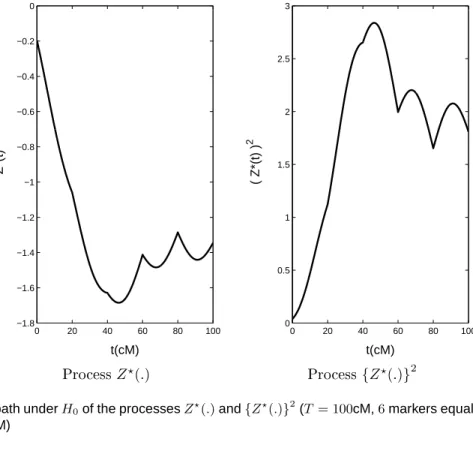
Fig. 1. A path under

H

0

of the processes

Z

⋆

(

.

)

and

{

Z

⋆

(

.

)

}

2

(

T

= 100

cM,

6

markers equally spaced

every

20

cM)

0

20 30 40

60 70 80

100

0.5

1

1.5

2

2.5

3

3.5

4

4.5

5

5.5

t(cM)

t*

1

=70cM and a

1

=4

t*

1

=30cM and a

1

=4

t*

1

=70cM and a

1

=6

0

20 30 40 50 60 70 80

100

3

3.5

4

4.5

5

5.5

6

6.5

7

7.5

8

t(cM)

a

2

=4

a

2

=6

m

= 1

m

= 2

,

t

⋆

1

= 30

M,

t

⋆

2

= 70

M,

a

1

= 4

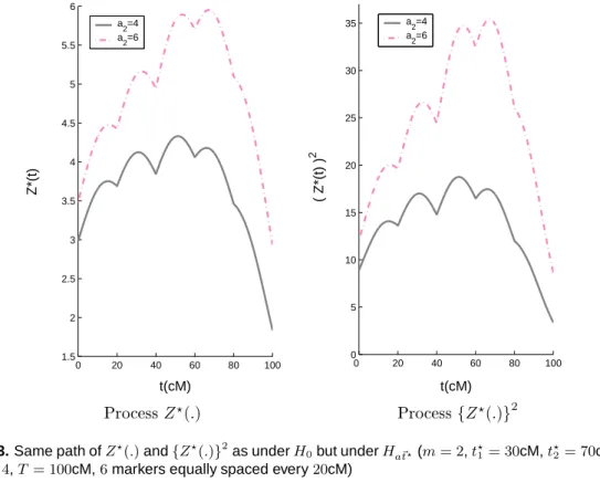
Fig. 2. Mean function

m

~

t

⋆

(

t

)

as a function of the number

m

of QTL, their positions

t

⋆

s

, and the

0

20

40

60

80

100

1.5

2

2.5

3

3.5

4

4.5

5

5.5

6

t(cM)

Z*(t)

a

2

=4

a

2

=6

0

20

40

60

80

100

0

5

10

15

20

25

30

35

t(cM)

( Z*(t) )

2

a

2

=4

a

2

=6

Proess

Z

⋆

(

.

)

Proess

{

Z

⋆

(

.

)

}

2

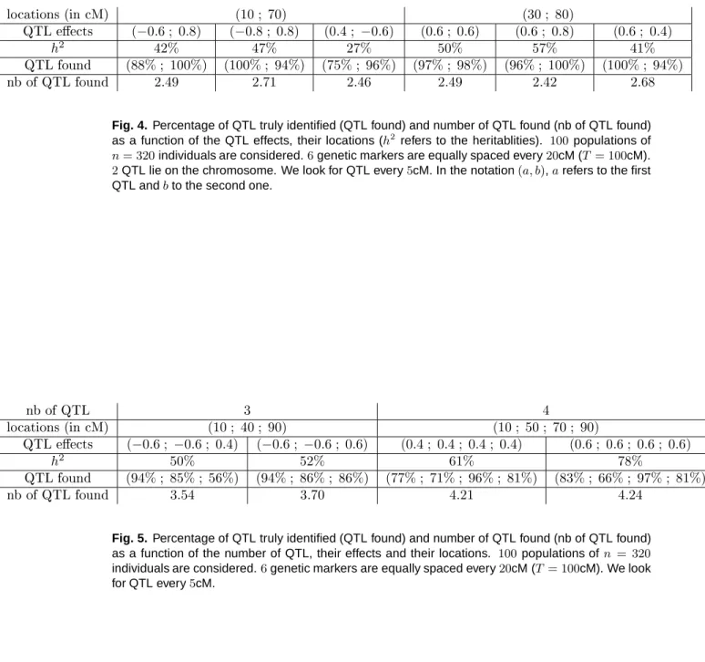
Fig. 3. Same path of

Z

⋆

(

.

)

and

{

Z

⋆

(

.

)

}

2

as under

H

0

but under

H

a~

t

⋆

(

m

= 2

,

t

⋆

1

= 30

cM,

t

⋆

2

= 70

cM,

In order to illustrate the theorem, we will onsider a geneti map whih onsists of

a hromosome of size

T

= 100

M with

6

markers equally spaed every

20

M. Figure 1 refersto theabsene of QTLon thehromosome. On theleft-side, a pathof theproess

Z

⋆

(

.

)

is represented under

H

0

. As there is not any QTL, it orresponds only to noise. Besides, we an observe the interpolation obtained between geneti markers. The same

pathorrespondingtotheproess

{

Z

⋆

(

.

)

}

2

hasbeenaddedontheright-side: in genetis,

we all this path "a likelihood prole". It is usually this path that we obtain when we

analyzedata. Note that manyauthors, insteadof omputing theproess

Λ

n

(

.

)

, fous on theLOD proess,

LOD

n

(

.

)

where

LOD

n

(

.

) = Λ

n

(

.

)

/

{

2 log(10)

}

.

Figure 2 represents the signal. On the left-side, we present some mean funtions

m

~

t

⋆

(

t

)

whenonly oneQTL(

m

= 1

)is loated onthehromosome. As expeted, the supremum ofthese interpolatedfuntions is obtainedatthe loationofthe QTL.Besides, thelarger

theQTLeetis,thestrongerthesignalis. Ontheright-side,thefousison

m

~

t

⋆

(

t

)

when

m

= 2

. Aording to the theorem,

m

~

t

⋆

(

t

)

is obtained by summing the mean funtions orrespondingto the ase

m

= 1

. As aonsequene,thefuntions

m

~

t

⋆

(

t

)

of the graphof theright-sideareeasilyobtainedfromthoseofthegraphoftheleft-side. Let'sfousonthe

urveinsolidline. ThetwoQTLareloatedrespetivelyat

t

⋆

1

= 30

Mand

t

⋆

2

= 70

M.So, themarkerinterval(

40

M,

60

M) isadjaenttothe twomarkerintervalswhere theQTL areloated. Asaresult,wean observeonthegraphthat thebiggestpeakis obtainedin

theinterval(

40

M,

60

M)andthatthesupremumisobtainedin themiddleof thismarker interval, at

50

M. Note that it is obtainedexatlyat

50

M sine we onsider exatlythe same eet (

a

1

=

a

2

= 4

) and that there is symmetry due to the loation of the QTL andthelength ofthehromosome. Ifnowweonsider alargereet fortheseond QTL

(

a

2

= 6

)loatedat

t

⋆

2

= 70

M(dashedline),weanobservealmostthesametwopeaksin theintervals(

40

M,

60

M)and(

80

M,

100

M).Besides,thesupremumofthemeanfuntion is obtainedat

52

M. It is like abaryenter : someweights are aeted to the QTL asa funtionoftheireets,sothesignalandtheloationofthesupremumisaetedbythese

weights.

Figure3istheanalogousofFigure1under thealternativeof

2

QTLloatedat

t

⋆

1

= 30

M and

t

⋆

2

= 70

M. As in Figure 1, the path of theproess

Z

⋆

(

.

)

is on the left-side whereas

theoneorrespondingto

{

Z

⋆

(

.

)

}

2

isontheright-side. Aordingto thetheorem, inorder

to obtainthe path of

Z

⋆

(

.

)

under

H

a~

t

⋆

, wehave to sum thepath of

Z

⋆

(

.

)

under

H

0

(ie. the noise), and the mean funtion

m

~

t

⋆

(

t

)

(ie. the signal). In other words, the path of

Z

⋆

(

.

)

under

H

a~

t

⋆

hasbeenobtainedbyaddingthepathof

Z

⋆

(

.

)

presentedinFigure1and

themean funtion of the graphof theright-sideof Figure 2. Note that on theright-side

of Figure 3, the likelihood prole (ie. the path of

{

Z

⋆

(

.

)

}

2

) haseasily been obtained by

omputationof thesquare of

Z

⋆

(

.

)

. We anobservein Figure3that, whenthe eetsof

thetwoQTLarethesame(ie. thesolidlines),thebiggestpeakisobtainedbetween

40

M and

60

MwhihisamarkerintervalwherethereisnoQTL:suhapeakisalledaghost QTL(MartinezandCurnow(1992)). Itwasexpetedsinethesupremumofthesignalwas

obtainedat

50

M.

Notethat whenweinreasetheeetoftheseondQTL(ie. thedashedlines),thebiggest

peakis obtainedin themarkerinterval(

60

M,

80

M)whihistheintervalwhihontains theseond QTL.Itis dueto thenoisesinethesignalisalmost thesameinthe intervals

(

40

M,

60

M) and (

60

M,

80

M) whereas the values of

Z

⋆

(

.

)

are larger under

H

0

in the markerinterval(

60

M,

80

M)thanintheinterval(

40

M,

60

M).

detetion, are the results of two omponents : the noise and the signal whih ontains

informationson thenumberof QTL, theireets and positions. Besides, when twoQTL

areloatedin twodierentmarkersintervalslosebut notadjaent,aghost QTLisoften

foundbetweenthese twomarkersintervals: itisdue tothesignal(f. Figure2). Wean

onlysayoften" beauseofthenoisewhihaetsalsothelikelihoodproles.

5.

A new method for QTL detection

Inthissetion,thegoalistoproposeamethodtoestimatethenumberofQTL,theireets

andtheirpositionsombiningresultsofthetheorem andapenalizedlikelihoodmethod.

5.1.

Introducing our method

Aordingtothetheorem, ifwedisretizethe soreproess atmarkerspositions, wehave

when

n

islarge:

~

S

n

=

m

~

~

t

⋆

+

~ε

where

S

~

n

= (

S

n

(

t

1)

, S

n

(

t

2)

, ... , S

n

(

t

K

))

′

,

m

~

~

t

⋆

= (

m

~

t

⋆(

t

1)

, m

~

t

⋆

(

t

2)

, ... , m

~

t

⋆

(

t

K

))

′

and

~ε

∼

N

(0

,

Σ)

with

Σ

kk

′

=

e

−

2

|

t

k

−

t

k

′

|

.

It willbeuseful to deorrelatetheomponentsof

S

~

n

forrunningthe penalizedlikelihood method. That'swhy,weproposetokeeponlypointsoftheproesstakenatmarkerpositions

: wean perform aCholesky deomposition of

Σ

(weremind that

S

n

is an interpolated proess"). However,wewill lookforQTLnotonlyonmarkerspostions.

Letonsider theCholeskydeomposition

Σ =

AA

′

. Itomes:

A

−

1

S

~

n

=

A

−

1

B

a

1

σ

, ... ,

a

m

σ

′

+

A

−

1

~

ε

where

B

isamatrixofsize

K

×

m

suhas

B

ks

=

e

−

2

|

t

k

−

t

⋆

s

|

.

Theproblemis that thenumber

m

ofQTLand theirpositions

t

⋆

1

,...,

t

⋆

m

are unknown. So, weonsideranewdisretizationof

[0

, T

]

orrespondingtoalltheloationswherewethink theQTLan beloated :

0

6

˜

t

1

<

˜

t

2

< ... <

˜

t

L

6

T

.

˜

a

1

, ...,

˜

a

L

will bethe orresponding eetsdividedby

σ

. As aonsequene,weanrewritethemodel:

A

−

1

S

~

n

=

A

−

1

B

˜

(˜

a

1

, ... ,

a

˜

L

)

′

+

A

−

1

~ε

(4)

where

B

˜

isamatrixofsize

K

×

L

suhas

B

˜

kl

=

e

−

2

|

t

k

−

˜

t

l

|

.

Atthis time, wewould liketo know whih of the oeients

˜

a

1

, ...,

˜

a

L

are exatly

0

: it willtellus wheretheQTLareloated. Asaonsequene,anaturalapproahistousethe

LASSOTibshirani(1996):

argmin

(˜

a

1

,...,

a

˜

L)

′

A

−

1

S

~

n

−

A

−

1

B

˜

(˜

a

1

, ... ,

˜

a

L

)

′

2

providedthat

|

a

˜

1

|

+

...

+

|

a

˜

L

|

6

ζ

ζ

is a tuning parameter. It will ontrol the amount of shrinkage that is applied to the estimatesTibshirani(1996). A large(resp. small)

ζ

will leadtothe estimationof alarge (resp. small)numberofQTL

m

. Wewillestimate

ζ

usingrossvalidationasdesribedin

5.2.

Computing the score and the Wald processes

Inorder to run ourmethod, weneed to alulate the soreproess disretized at marker

loations. Weremindthat

t

k

referstotheloationofmarker

k

. AordingtoRabier(2010), thesorestatistionmarker

k

veries:

S

n

(

t

k

) =

n

X

j

=1

(

y

j

−

µ

)

2 1

X

j(

t

k)=1

−

1

σ

√

n

(5)

AordingtoProhorovandbyontiguity(f. Setion 7.1),thesoretest anbeobtained,

replaing

µ

by

y

¯

:=

P

n

j

=1

y

j

/n

and

σ

by

n

1

n

−

1

P

n

j

=1

(

y

j

−

y

¯

)

2

o

1

/

2

.

Besides, let

W

n

(

.

)

the Wald proess for

n

observations. As the model is regular and by ontiguity, we have

∀

t

∈

[0

, T

]

,

S

n

(

t

) =

W

n

(

t

) +

o

P

(1)

where

o

P

(1)

is asequene whih onvergesto

0

in probabilityunder

H

0

and

H

a~

t

⋆

.

As a onsequene, ourmethod for QTL detetion is also suitable with the Wald proess

W

n

(

.

)

(justreplae

S

n

by

W

n

in Setion5.1). Inthisase,aordingto Rabier(2010):

W

n

(

t

k

) =

n

q/

ˆ







n

X

j

=1

(

y

j

−

y

¯

)

2







1

/

2

where

q

ˆ

isthemaximumlikelihoodestimatorof

q

.

5.3.

How to improve our method

Ourmethodis basedontheasymptotiresultofthetheorem. Asaonsequene,wehave

to onsideranumberof observations

n

largeenoughto run themethod. Weremindthat wehave

n

observations sineweonsider

n

individuals. On theother hand,in themodel (4),wehavethistimeonly

K

observationswhihorrespondtothesorestatisti(obtained fromthe

n

individuals)onmarkersand deorrelated. Besides,there are

L

parameters

˜

a

1

, ...,

˜

a

L

toestimate(ifweexept

ζ

). Weremindthat

˜

t

1

,... ,

˜

t

L

denotetheloationwhere we aregoingto lookforQTL.Inmostofases,aswedon'thaveanyideawheretheQTLare

lying,wewilllookforQTLonmarkersandbetweenmarkers. Ifweonsider

d

positionsin eah markerinterval, then

L

=

K

(

d

+ 1)

−

d

. Itomes

L >> K

. Insuh asituation,the LASSOissuitable. Howewer,inordertoimprovetheperformaneoftheLASSO,itwould

benieifweoulddealwithalargenumberofobservations

K

. Theproblemisthat

K

refers tothenumberofgenetimarkerwhih isonstant. So,wehaveto ndanalternative. In

anasymptotistudy,thequestionisalwaysthesame: howmanyindividuals

n

areneeded to reah theasymptoti ? We haveto keep in mind that even if

n

is verylarge, wewill onlydealwith

K

observations(ie. thenumberof markers) in model (4). As aresult, we proposetosplit theindividuals intogroupsandto analyzethese groupsseparately,thatis

to sayomputing thesore(or Wald)proess foreahgroup. Obviously,wehaveto deal

withanumberofindividualslargeenoughineahgroupin ordertoreahtheasymptoti.

Weonsidergroupsofsamesizesandweall

I

thenumberofgroups:

n/I

isthenumberof individualsin eah group.

S

i

I

(

.

)

denotesthesoreproessfor the

i

thgroup. Aordingto thetheorem,

S

i

I

(

.

)

isasymptotiallythesquareofanonlinearinterpolatedproess"with ameanfuntion

m

~

~

t

⋆

,I

(

.

)

underthealternative,verifying

m

~

t

⋆

,I

(

t

) =

n

α

(

t

)

m

~

t

⋆

,I

(

t

ℓ

) +

β

(

t

)

m

~

t

⋆

,I

(

t

r

)

o

/

r

E

h

{

2

p

(

t

)

−

1

}

2

i

where

m

~

t

⋆

,I

(

t

ℓ

) =

L

X

s

=1

a

s

e

−

2

|

t

⋆

s

−

t

ℓ

|

/

(

σ

√

I

)

,

m

~

t

⋆

,I

(

t

r

) =

L

X

s

=1

a

s

e

−

2

|

t

r

−

t

⋆

s

|

/

(

σ

√

I

)

Note that

√

I

at the denominator omes from the fat that the QTL eets have been denedasafuntion ofthetotalnumberofindividuals

n

.

So,sinethe groupsare independent,weaneasilyadapt ourmethod of Setion5.1. We

havenow:

~

S

1

I

, ... , ~

S

I

I

′

=

m

~

~

t

⋆

,I

, ... , ~

m

~

t

⋆

,I

′

+ (

~ε

1

, ... , ~ε

I

)

′

where

m

~

~

t

⋆

,I

=

m

~

t

⋆

,I

(

t

1)

, m

~

t

⋆

,I

(

t

2)

, ... , m

~

t

⋆

,I

(

t

K

)

,

S

~

i

I

=

S

I

i

(

t

1)

, S

I

i

(

t

2)

, ... , S

I

i

(

t

K

)

and

~ε

i

iidofsize

1

×

K

suhaseah

~ε

i

∼

N

(0

,

Σ)

with

Σ

kk

′

=

e

−

2

|

t

k

−

t

k

′

|

.

Inthesamewayaspreviously(f. Setion 5.1)providedthat this time

a

˜

1

, ...,

˜

a

L

are the eetsdividedby

σ

√

I

:

Γ

S

~

1

I

, ... , ~

S

I

I

′

= Ξ (˜

a

1

, ... ,

˜

a

L

)

′

+ Γ

~ε

(6)

Γ

isasquarematrixofsize

KI

suhas

Γ =

Diag

A

−

1

, ... , A

−

1

.

Ξ

isaolumn vetorofomponents

A

−

1

B

˜

repliated

I

times. Toonlude,weproposetousetheLASSOTibshirani (1996):

argmin

(˜

a

1

,...,

˜

a

L)

′

Γ

~

S

I

1

, ... , ~

S

I

I

′

−

Ξ (˜

a

1

, ... ,

˜

a

L

)

′

2

providedthat

|

˜

a

1

|

+

...

+

|

a

˜

L

|

6

ζ

6.

Simulations

Inthis Setion, weperformour methodusing Wald proesses(f. Setion 5.2) and5fold

rossvalidationfortheLASSO.Weonsider

100

populationsofsize

n

= 320

. Weusemainly MATLABtoperformourmethod. WeusedRtoperformTheLASSOwithpakageLARS

ofHastieandEfron. CompositeIntervalMappingwasperformedusing(R/qtlBromanand

al.(2003)).

6.1.

How does our method perform?

In order to illustrate the performanes of our method, we onsider a sparse map whih

onsists of

6

genetimarkersequallyspaed every

20

M on ahromosomeof length

T

=

100

M. Welook fora QTL every

5

M. Inorder to make groups,wehave to nd agood ompromisebetweenhavingenoughindividualsineahgrouptoreahtheasymptoti,and

havingalargenumberofgroupstoinreasetheperformanesoftheLASSO.Wesplithere

our

320

individuals into

8

groups of

40

individuals in order to improve the method (f. Setion 5.3). Indeed, it is reasonable to onsider the asymptoti to be reahed with

40

individuals(Rabier(2010)).Asaonsequene,wehavenow

L

= 21

parameterstoestimate with

6

×

8 = 48

observations(

6

markersand

8

groups).

Westudyseveralsituationswith

2

,

3

and

4

QTL.WewillsaythataQTListrulyidentied iftheQTLis ndinaneighbourhood of

5

M ofthetrueposition (iean intervaloflength

10

Menteredonthetrueloation). Besides,inordertoountthenumberofQTLfound, wehavehoosen notto penalizeifseveralQTLwerefoundin the

10

Mintervalsentered onthetrueloations,whereaswehavehoosentopenalizealotforanyQTLfoundoutside

oftheintervals. Asaonsequene,weountonlyoneQTLif

2

or

3

QTLarefoundin the

10

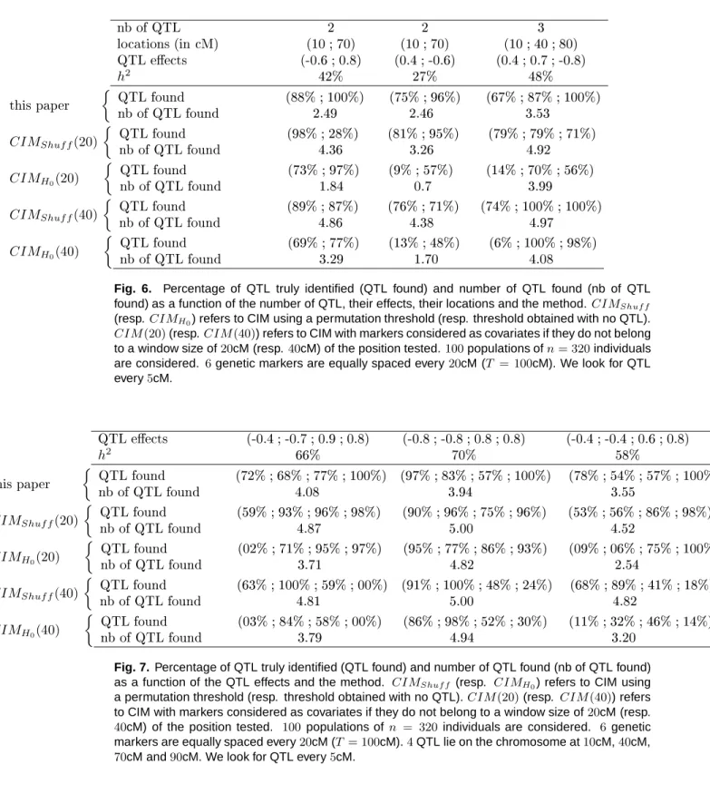
MintervalsenteredonthetrueloationsandweountoneQTLforeveryQTLfound outsidetheseintervals.

In Figure 4, we study a situation with

2

QTL loated on the hromosome. First, two QTLlinked in repulsion (iewith opposite signs)areloatedat positions

10

M and

70

M onthehromosome. Wehaveto keepin mind that asourmethod isbasedonontiguity,

theQTLeets haveto belose to

0

. However,weansee in Figure4, that themethod givesgoodresultsevenwhentheeets arenotsoloseto

0

. Note thattheheritabilityis indiatedjust forinformationbut itis notlinkedto theperformanesofourmethod sine

thebiggertheeetsarethebiggertheheritabilityis. ThenumberofQTLfoundisslightly

greaterthan

2

,but itisreasonablesinewepenalizealotwhenweareoutsideoftheQTL intervals. We obtain thesame onlusions forthe two QTL linked in oupling (ie. with

samesigns)presentedontherightsideofFigure4. Goodperformanesofthemethodsare

alsoillustratedin Figure5when

3

and

4

QTLareloatedonthehromosome.

6.2.

Comparison with the Composite Interval Mapping

Weproposehereto ompare ourmethod with theComposite IntervalMapping(CIM) of

Jansen (1993) and Zeng (1994), largelyused in the geneti ommunity. Weremind that

CIMonsistsin ombiningintervalmappingontwoankingmarkersandmultiple

regres-sionanalysisonotherseletedmarkers(Wuandal.(2007)). Thisway,theQTLnotloated

inthemarkerintervaltesteddon'taettheteststatistisanymore. Asaonsequene,itis

possibletoperformseparatelyintervalmappingineahmarkerintervaltotestthepresene

ofaQTLintheinterval. However,thehoieofthemarkersasofatorsisveryempirial

: wedon'tknowhowtohoiethesetofmarkersin amathematialpointofview.

FortheomparisonbetweenourmethodandCIM,weusethesameongurationasin

Se-tion6.1. Westudyseveralsituationswith

2

,

3

and

4

QTLonthehromosome(seeFigures 6and7). Weompute

4

kindsofCIM.First,weonsidertwowaysofhoosingtheofators :

CIM

(20)

(resp.

CIM

(40)

) referstoCIM with markersonsidered asovariatesif they donotbelongto awindowsize of

20

M(resp.

40

M)ofthepositiontested. Seondly, we onsidertwowaysofomputingthethresholds: oneobtainedusing

1000

permutationsand alled

Shuf f

here(Churhilland Doerge(1994)),andanotherwhihisobtained theoreti-allyunder

H

0

(

6

.

76

aordingtoRabier(2010)).

InordertoountthenumberofQTLforCIM,foreahmarkerinterval,weountoneQTL

ifthe supremumof theproess is abovethethreshold (itorresponds to thedenition of

CIM).Besides, forCIM,wewillsaythat aQTListruly identiediftheQTL isndin a

neighbourhoodof

5

Mofthetrueposition. Forinstane,ifaQTLisloatedat

10

M, the supremuminthemarkerinterval(

0

M;

20

M)hastobeobtainedbetween

5

Mand

15

M. Howewer,ifweonsideraQTLloatedat

40

M(ieonthethirdmarker),wewillonsider thatthisQTListrulyidentiedifthesupremuminthemarkerinterval(

20

M;

40

M)is ob-tainedbetween

35

Mand

40

M,orifitisobtainedbetween

40

Mand

45

Minthemarker interval(

40

M;

60

M).

AordingtoFigure 6,ifweonsider

2

QTLat

10

M and

70

M witheets

−

0

.

6

and

0

.

8

, weansee that

CIM

H

trueQTLarelargelyfound. However,ifweonsiderthesame

2

QTLbutwith eets

0

.

4

and

−

0

.

6

,

CIM

H

0

(20)

performs badly.

CIM

Shuf f

(20)

seemsto the best way to perform CIM : thetrue QTL arelargely found but wend

3

.

26

QTL.If weonsider

3

QTL, the best wayto perform CIMis

CIM

Shuf f

(40)

but we nd

4

.

97

QTL.As aonsequene,the hoieoftheofatorsandthehoieofthethresholdshighlydependsoftheonguration

: CIMisveryempirial. Ifnowwehavealookonourmethodin Figure6,weobtainnie

results: theQTL are largelyfound and thenumber ofQTL found is good whateverthe

ongurationstudied. Sameonlusions holdwith

4

QTL(seeFigure7).

6.3.

Our method is not affected by epistasis

Until now, wehavesupposed that theQTLeets wereadditivesand that there were no

interation betweenthem (f. Setion 2). However,there are many interations between

loi in the genome (ie. epistasis). That's why wepropose here to integrate interations

in themodelonsidered. Weremindthat

m

referto the number ofadditiveQTL and

q

s

to theQTL eet ofthe sth additive QTL.Its position is

t

⋆

s

. We will all

m

˜

thenumber of interations and

q

˜

s

the eet of the sthinteration. Theloi orresponding to thesth interationwillbealled

˜

t

2

s

−

1

and

t

˜

2

s

. Inthisontext,thequantitativetrait

Y

veries:

Y

=

µ

+

m

X

s

=1

X

(

t

⋆

s

)

q

s

+

˜

m

X

s

=1

X

(˜

t

2

s

−

1)

X

(˜

t

2

s

) ˜

q

s

+

σε

where

ε

isaGaussian whitenoise. Weintroduetwonewhypothesis:

H

a~

t

⋆

, b

t

˜

: thereare

m

additiveQTLloatedrespetivelyat

t

⋆

1

,...,

t

⋆

m

and witheet

q

1

=

√

a

1

n

,...,

q

m

=

a

m

√

n

where

(

a

1

, ..., a

m

)

∈

R

m⋆

andthereare

m

˜

interations: betweenloi

˜

t

1

and

˜

t

2

,...,betweenloi

˜

t

2 ˜

m

−

1

and

˜

t

2 ˜

m

,with eetsrespetively

q

˜

1

=

b

1

√

n

,...,

q

˜

m

˜

=

b

m

˜

√

n

where

(

b

1

, ..., b

m

˜

)

∈

R

˜

m⋆

".

H

0

, b

˜

t

: thereisnotanyadditiveQTLon

[0

, T

]

andthereare

m

˜

interations: betweenloi

˜

t

1

and

˜

t

2

,...,betweenloi

˜

t

2 ˜

m

−

1

and

˜

t

2 ˜

m

,with eetsrespetively

q

˜

1

=

b

1

√

n

,...,

q

˜

m

˜

=

b

m

˜

√

n

where

(

b

1

, ..., b

m

˜

)

∈

R

˜

m⋆

". PropositionUnder

H

0

, b

t

˜

andunder

H

a~

t

⋆

, b

˜

t

∀

k S

n

(

t

k

) =

Z

⋆

(

t

k

) +

o

P

(1)

and

Λ

n

(

t

k

) =

{

Z

⋆

(

t

k

)

}

2

+

o

P

(1)

where

Z

⋆

(

.

)

istheGaussianproessofthetheorem(f. Setion4.1)suhas

Z

⋆

(

.

)

isentered

under

H

0

, b

˜

t

andwith the meanfuntion

m

~

t

⋆

(

.

)

ofthe theorem under

H

a~

t

⋆

, b

˜

t

.

TheproofisgiveninSetion 7.2. Aordingtotheproposition,ourmethodwhihisbased

onlyonpointsoftheproesstakenatmarkerpositions,isnotaetedbyepistasis. Indeed,

under

H

a~

t

⋆

, b

˜

t

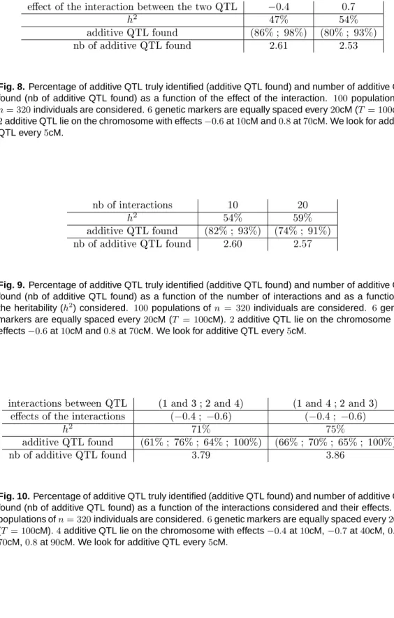
,themeanfuntionat markerpositionisthesameaspreviously.

Figures 8 to 11 illustrate this phenomenon. The same map aspreviously is onsidered.

In Figures 8 and 9, weonsider twoadditive QTL on thehromosome : one with eet

−

0

.

6

at

10

Mandtheotherwitheet

0

.

8

at

70

M.Tobegin,inFigure8,weonsiderone interation: wehavehoosentostudyaninterationbetweenthetwoQTL.Weonsidertwo

foundandthenumberofadditiveQTLfound isgood. Then, inFigure9,weonsiderthis

time

10

and

20

interations(keepingtheinterationbetweentheQTLwitheet

−

0

.

4

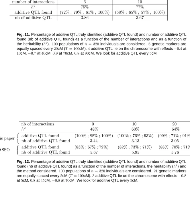
). The resultsarestillnie: theperformanesofourmethodarenotaetedbytheinterations(as

expeted withtheProposition). Same onlusionshold with

4

additiveQTL(seeFigures 10and11). Note thatforFigure11,wekeptthesameinterationbetweenQTLasonthe

leftsideofFigure10,andweaddedotherinterations.

6.4.

Our method is suitable for dense map

Toonlude,wewould liketo mentionthat ourmethod isalsosuitable fordensemap (ie

alargenumberof genetimarkersloseto eah other). Inthisase, wewill perform only

testsongenetimarkers. InFigure12,weonsider,aspreviously,ahromosomeoflength

T

= 100

M, butgenetimarkersarenowloatedevery

5

M.WelookforQTLevery

5

M. We ompare here our method and a lassial LASSO method whih onsists of a linear

model where thetrait

Y

is thevariableto explain andthe regressorsarethe markers. In ordertoperformthelassialLASSO,weused

0

.

1

asatuningparameterinsteadof

5

fold ross-validation. It wasa good ompromise (betweenthe QTL found and their number)

sine the results of the ross-validation were not good at all. Aording to the Figure

(usingthesamerulestollthetableasin Setion6.1), weansee thatourmethod gives

largelybetterresultsthanthelassialLASSO.Notethatourmethodisstilltheoretially

unaetedbyanyinterations.

7.

Proofs

7.1.

Proof of the theorem

We will onsider values

t

,

t

⋆

1

, ...,

t

⋆

m

of the parameters that are distint of the markers positions, andtheresultwillbeprolongedbyontinuityatthemarkerspositions.

Study under

H

0

:

ThereisnoQTLonthehromosome. TheproofisfullygiveninRabier(2010).

Nevertheless, weremindthat thesoreteststatistifor

n

observations veriesat position

t

:

S

n

(

t

) =

n

X

j

=1

(

y

j

−

µ

) (2

p

j

(

t

)

−

1)

σ

√

n

r

E

h

{

2

p

(

t

)

−

1

}

2

i

(7) where

E

h

{

2

p

(

t

)

−

1

}

2

i

=

{

α

(

t

)

}

2

+

{

β

(

t

)

}

2

+ 2

α

(

t

)

β

(

t

)

e

−

2(

t

r

−

t

ℓ

)

.

Itwillbeusefulforthestudyofthegeneralalternative.

Study under

H

a~

t

⋆

:

Thereare severalQTLloated onthehromosome. Wesuppose that theQTLeetsare

additivesandthatthere isnointerationbetweenthem.

Inthis ontext,thequantitativetrait

Y

veries:

Y

j

=

µ

+

m

X

s

=1

X

j

(

t

⋆

s

)

q

s

+

σε

j

(8)

•

ξ

: numberof Markerintervals"whihontaintheQTL.

γ

= 1

, ..., ξ

willrefertothedierentintervals.

•

m

γ

: numberofQTLintheinterval

γ

.

τ

= 1

, ..., m

γ

referstothe

τ

thQTLintheinterval

γ

.

•

the

s

thQTLon

[0

, T

]

,anberewritten,

s

= (

τ, γ

) =

n

P

γ

−

1

i

=1

m

i

o

+

τ

Let

θ

a~

t

⋆

= (

q

1

, ..., q

m

, µ, σ

)

and

θ

0

~

t

⋆

= (0

, ...,

0

, µ, σ

)

. Aftersomealulations,thelikelihoodof

Y, X

n

t

⋆ℓ

(1

,

1)

o

, X

n

t

⋆r

(1

,

1)

o

, ..., X

n

t

⋆ℓ

(1

,ξ

)

o

, X

n

t

⋆r

(1

,ξ

)

o

withrespettothemeasure

λ

⊗

N

⊗

...

⊗

N

,

λ

beingtheLebesguemeasure,

N

theounty measureon

N

, veries:

L

⋆

(

θ

a~

t

⋆

) =

X

(

u

1

,...,u

m)

∈{−

1

,

1

}

m

f

(

µ

+

u

1

q

1

+

...

+

u

m

q

m

,σ

)(

y

)

×

(

ξ

Y

γ

=1

A

n

t

⋆ℓ

(

τ,γ

)

, t

⋆

(

τ,γ

)

o

"

m

γ

−

1

Y

τ

=1

R

n

t

⋆

(

τ,γ

)

, t

⋆

(

τ

+1

,γ

)

o

#

A

n

t

⋆r

(

m

γ

,γ

)

, t

⋆

(

m

γ

,γ

)

o

!

g

⋆

(

~t

⋆

)

)

where

u

s

=

u

(

τ,γ

)

A

n

t , t

⋆

(

τ,γ

)

o

=

r

n

t , t

⋆

(

τ,γ

)

o

1

X

(

t

)

u

(

τ,γ

)=

−

1

+ ¯

r

n

t , t

⋆

(

τ,γ

)

o

1

X

(

t

)

u

(

τ,γ

)=1

R

n

t

⋆

(

τ,γ

)

, t

⋆

(

τ

+1

,γ

)

o

= ¯

r

n

t

⋆

(

τ,γ

)

, t

⋆

(

τ

+1

,γ

)

o

1

u

(

τ,γ

)

u

(

τ

+1

,γ

)=1

+

r

n

t

⋆

(

τ,γ

)

, t

⋆

(

τ

+1

,γ

)

o

1

u

(

τ,γ

)

u

(

τ

+1

,γ

)=

−

1

g

⋆

(

~t

⋆

) =

1

2

ξ

−

1

Y

γ

=1

D

n

t

⋆r

(

m

γ

,γ

)

, t

⋆ℓ

(1

,γ

+1)

o

D

(

t, t

′

) = ¯

r

(

t, t

′

) 1

X

(

t

)

X

(

t

′

)=1

+

r

(

t, t

′

) 1

X

(

t

)

X

(

t

′

)=

−

1

Thelikelihood

L

⋆

n

(

θ

a~

t

⋆

)

for

n

observationsisobtainedbytheprodutof

n

termsasabove. Let

Q

n

and

P

n

twosequenesofprobabilitymeasuresdenedonthesamespae

(Ω

n

,

A

n

)

.

Q

n

(respetively

P

n

)isthelaworrespondingto thedensity

L

⋆

n

(

θ

a~

t

⋆

)

(resp

L

⋆

n

(

θ

0

~

t

⋆

)

). We willalltheloglikelihoodratio

log

dQ

n

dP

n

. Itveries:

log

dQ

n

dP

n

= log

n

L

⋆

n

(

θ

a~

t⋆

)

L

⋆

n

(

θ

0

~

t⋆

)

o

.

Asthemodelisdierentiablein quadratimeanat

θ

a~

t

⋆

and aordingtotheentral limit theorem:

log

dQ

n

dP

n

H

0

→

N

(

−

1

2

ϑ

2

, ϑ

2

)

with

ϑ

2

∈

R

+

⋆

Bytheiii)ofLeCam'srstlemma,wehave

Q

n

⊳ P

n

. Let

o

P

θ

0

(1)

beshortforasequeneofrandomvetorsthatonvergestozerosinprobability

under

H

0

(i.e. noQTLonthewholeintervalstudied). Besides,aordingto Rabier(2010):

where

S

n

(

t

)

isgivenin formula(7). Let

o

P

θ

₀

~

t⋆

(1)

beasequeneofrandomvetorsthatonvergestozerosifthereisnoQTLat

t

⋆

1

,...,

t

⋆

m

. Then,itislearthat :

Λ

n

(

t

) =

{

S

n

(

t

)

}

2

+

o

P

θ

₀

~

t⋆

(1)

Let

o

P

θ

a~

t⋆

(1)

beasequeneofrandomvetorsthat onvergestozerosifthereare

m

QTL at

t

⋆

1

,...,

t

⋆

m

. As

Q

n

⊳ P

n

, aordingtoiv)ofLeCam'srstlemma :

Λ

n

(

t

) =

{

S

n

(

t

)

}

2

+

o

P

θ

a~

t⋆

(1)

So,alulationsanbedonewiththesoreteststatisti.

Aordingto Rabier(2010), the sore test statisti at

t

anbe obtainedby a non linear interpolation:

S

n

(

t

) =

α

(

t

)

S

n

(

t

ℓ

) +

β

(

t

)

S

n

(

t

r

)

r

E

h

{

2

p

(

t

)

−

1

}

2

i

where

α

(

t

) =

Q

1

,

1

t

+

Q

1

,

−

1

t

−

1

and

β

(

t

) =

Q

1

,

1

t

−

Q

1

,

−

1

t

. Let

m

~

t

⋆

(

.

)

betheasymptotimeanfuntionofthesoreproess

S

n

(

.

)

. Itomes :

m

~

t

⋆

(

t

) =

α

(

t

)

m

~

t

⋆

(

t

ℓ

) +

β

(

t

)

m

~

t

⋆

(

t

r

)

r

E

h

{

2

p

(

t

)

−

1

}

2

i

Letalulate thequantities

m

~

t

⋆

(

t

ℓ

)

and

m

~

t

⋆(

t

r

)

.

Weremindthat

t

k

referstotheloationofmarker

k

. AordingtoRabier(2010),thesore statistionmarker

k

veries:

S

n

(

t

k

) =

n

X

j

=1

(

y

j

−

µ

)

2 1

X

j(

t

k)=1

−

1

σ

√

n

Aordingto formula(8):

S

n

(

t

k

) =

1

√

n

n

X

j

=1

ε

j

2 1

X

j(

t

k)=1

−

1

+

1

σn

n

X

j

=1

(

m

X

s

=1

X

j

(

t

⋆

s

)

a

s

)

2 1

X

j

(

t

k)=1

−

1

=

S

0

n

(

t

k

) +

1

σn

n

X

j

=1

(

m

X

s

=1

X

j

(

t

⋆

s

)

a

s

)

2 1

X

j

(

t

k)=1

−

1

(9) where

S

0

n

(

t

k

)

isthesoreobtainedunder

H

0

atloation

t

k

. Bythelawoflargenumber:

1

n

n

X

j

=1

(

m

X

s

=1

X

j

(

t

⋆

s

)

a

s

)

2 1

X

j

(

t

k)=1

−

1

→

E

"(

m

X

s

=1

X

(

t

⋆

s

)

a

s

)

2 1

X

(

t

k)=1

−

1

#

Aordingto Rabier(2010),wehave:

E

"(

m

X

s

=1

X

(

t

⋆

s

)

a

s

)

2 1

X

(

t

k

)=1

−

1

#

=

m

X

s

=1

a

s

e

−

2

|

t

⋆

s

−

t

k

|

Itomes:

m

~

t

⋆

(

t

k

) =

1

σ

m

X

s

=1

a

s

e

−

2

|

t

⋆

s

−

t

k

|

Asaonsequene:

m

~

t

⋆

(

t

ℓ

) =

1

σ

m

X

s

=1

a

s

e

−

2

|

t

⋆

s

−

t

ℓ

|

,

m

~

t

⋆

(

t

r

) =

1

σ

m

X

s

=1

a

s

e

−

2

|

t

⋆

s

−

t

r

|

Weak onvergeneof the soreproess:

Theproofis exatlythesameasin Rabier(2010).

7.2.

Proof of the proposition

˜

m

is the number of interations and

q

˜

s

the eet of the sth interation. The loi orre-sponding tothesthinterationare

t

˜

2

s

and

t

˜

2

s

−

1

. Inthisontext,thequantitativetrait

Y

veries:

Y

=

µ

+

m

X

s

=1

X

(

t

⋆

s

)

q

s

+

˜

m

X

s

=1

X

(˜

t

2

s

−

1)

X

(˜

t

2

s

) ˜

q

s

+

σε

(10)

where

ε

isaGaussian whitenoise.

Wewill onsider valuesof

˜

t

1

, ...,

t

˜

2 ˜

m

and

t

⋆

1

, ...,

t

⋆

m

distintof markerpositions, and the resultwill beprolongedbyontinuity.

Let

o

P

θ

0

~

t⋆ ,

0˜

t

(1)

beasequeneofrandomvetorsthatonvergestozerosifthereisnoadditive

QTLat

t

⋆

1

, ...,

t

⋆

m

and nointerationsbetweenloi

˜

t

1

and

˜

t

2

, ....,nointerations between loi

˜

t

2 ˜

m

−

1

and

˜

t

2 ˜

m

. Inthesamewayasintheproofofthetheorem,itislearthat:

Λ

n

(

t

k

) =

{

S

n

(

t

k

)

}

2

+

o

P

θ

₀

~

t⋆ ,

0˜

t

(1)

where

S

n

(

t

k

)

isgiveninformula(5)ofSetion5.2.

Inordertoadapttheproofofthetheorem,wejusthavetoonsiderthelikelihoodof

Y

and theankingmarkersof theadditiveQTL(as previously)butwehaveto add theanking

markersof

t

˜

1

,...,

˜

t

2 ˜

m

. Themodelisstilldierentiableinquadratimean. Let

o

P

θ

a~

t⋆ ,b

˜

t

(1)

be a sequene of random vetors that onverges to zeros if there are

m

additiveQTL at

t

⋆

1

, ...,

t

⋆

m

and

m

˜

interations : loi

˜

t

1

and

˜

t

2

, ...., loi

˜

t

2 ˜

m

−

1

and

˜

t

2 ˜

m

. Then,aordingto iv)ofLeCam'srstlemma:

Λ

n

(

t

k

) =

{

S

n

(

t

k

)

}

2

+

o

P

θ

a~

t⋆ ,b

t

˜

(1)

Aordingto formula(10),wehave:

S

n

(

t

k

) =

1

√

n

n

X

j

=1

ε

j

2 1

X

j(

t

k)=1

−

1

+

1

σn

n

X

j

=1

(

m

X

s

=1

X

j

(

t

⋆

s

)

a

s

)

2 1

X

j

(

t

k)=1

−

1

+

1

σn

n

X

j

=1

(

m

˜

X

s

=1

X

j

(˜

t

2

s

−

1)

X

j

(˜

t

2

s

)

b

s

)

2 1

X

j

(

t

k)=1

−

1

=

S

0

n

(

t

k

) +

1

σn

n

X

j

=1

(

m

X

s

=1

X

j

(

t

⋆

s

)

a

s

)

2 1

X

j

(

t

k)=1

−

1

+

1

σn

n

X

j

=1

(

m

˜

X

s

=1

X

j

(˜

t

2

s

−

1)

X

j

(˜

t

2

s

)

b

s

)

2 1

X

j

(

t

k)=1

−

1

(11) where

S

0

n

(

t

k

)

isthesoreobtainedunderthenullhypothesisthatthereisnoadditiveQTL andnointerationson

[0

, T

]

(same

S

0

n

asinformula(9) oftheproofof thetheorem). A-ordingtotheproofof thetheorem, wehave

1

σn

P

n

j

=1

{

P

m

s

=1

X

j

(

t

⋆

s

)

a

s

}

2 1

X

j

(

t

k)=1

−

1

whihtendsto

m

~

t

⋆

(

t

k

)

. Besides,

1

σn

n

X

j

=1

(

m

˜

X

s

=1

X

j

(˜

t

2

s

−

1)

X

j

(˜

t

2

s

)

b

s

)

2 1

X

j(

t

k)=1

−

1

→

E

"(

m

˜

X

s

=1

X

(˜

t

2

s

−

1)

X

j

(˜

t

2

s

)

b

s

)

2 1

X

(

t

k)=1

−

1

#

Wehave:

E

X

(˜

t

2

s

−

1)

X

(˜

t

2

s

)

2 1

X

(

t

k)=1

−

1

= 2

E

X

(˜

t

2

s

−

1)

X

(˜

t

2

s

)1

X

(

t

k)=1

−

e

−

2

|

˜

t

2

s

−

˜

t

2

s

−

1

|

If

t

k

<

t

˜

2

s

−

1

<

˜

t

2

s

,then:

E

X

(˜

t

2

s

−

1)

X

(˜

t

2

s

)

2 1

X

(

t

k)=1

−

1

= 0

If

˜

t

2

s

−

1

< t

k

<

˜

t

2

s

,then:

E

X

(˜

t

2

s

−

1)

X

(˜

t

2

s

)

2 1

X

(

t

k

)=1

−

1

= 0

Asaonsequene:

E

X

(˜

t

2

s

−

1)

X

(˜

t

2

s

)

2 1

X

(

t

k)=1

−

1

= 0

Itonludestheproofforunder

H

a~

t

⋆

, b

˜

t

. Inordertoobtaintheresultunder

H

0

, b

˜

t

,wejust havetodealwithontiguity,onsidering thelikelihoodof

Y

andonlytheankingmarkers of

˜

t

1

, ...,

t

˜

2 ˜

m

(ie the loi for the interations). Then, we do the same alulations as in formula(11)but thistimethereis notanymoretheadditiveterm(ietheseond term). It

onludestheproofoftheProposition.

8.

Acknowledgements

The authors thank Jean-Mihel Elsen for having proposed this subjet of researh and

fruitfuldisussions. This work hasbeensupported bytheAnimalGeneti Departmentof

loations(inM)

(10 ; 70)

(30 ; 80)

QTLeets

(

−

0

.

6 ; 0

.

8)

(

−

0

.

8 ; 0

.

8)

(0

.

4 ;

−

0

.

6)

(0

.

6 ; 0

.

6)

(0

.

6 ; 0

.

8)

(0

.

6 ; 0

.

4)

h

2

42%

47%

27%

50%

57%

41%

QTLfound

(88% ; 100%)

(100% ; 94%)

(75% ; 96%)

(97% ; 98%)

(96% ; 100%)

(100% ; 94%)

nbofQTLfound

2

.

49

2

.

71

2

.

46<