An agent based early warning indicator
for financial market instability
Vidal-Tomás, David and Alfarano, Simone
Universitat Jaume I
24 October 2018
Online at
https://mpra.ub.uni-muenchen.de/89693/
(will be inserted by the editor)
An agent based early warning indicator for financial market instability.
David Vidal-Tom´as · Simone Alfarano
Received: date / Accepted: date
Abstract Inspired by the Bank of America Merrill Lynch Global Breath Rule, we propose an investor sentiment
index based on the collective movement of stock prices in a given market. We show that the time evolution of the
sentiment index can be reasonably described by the herding model proposed by Kirman on his seminal paper
“Ants, rationality and recruitment” (Kirman, 1993). The correspondence between the index and the model
allows us to easily estimate its parameters. Based on the model and the empirical evolution of the sentiment
index, we propose an early warning indicator able to identify optimistic and pessimistic phases of the market.
As a result, investors and policymakers can set different strategies anticipating financial market instability. The
former, reducing the risk of their portfolio, and the latter, setting more efficient policies to avoid the effect of
financial crashes on the real economy. The validity of our results is supported by means of a robustness analysis
showing the application of the early warning indicator in eight different stock markets.
JEL: G10 - C61 - D84
Keywords Herding behaviour· Kirman model·Financial market
David Vidal-Tom´as
Universitat Jaume I. Department of Economics, Castell´on, Spain E-mail: [email protected]
Simone Alfarano
“I define a speculative bubble as a situation in which news of price increases spurs investor enthusiasm,
which spreads by psychological contagion from person to person, in the process amplifying stories that might
justify the price increases and bringing in a larger and larger class of investors, who, despite doubts about
the real value of an investment, are drawn to it partly through envy of others’ successes and partly through a
gambler‘s excitement”. (Robert J Shiller, Irrational Exuberance, 2015)
1 Introduction
Traditional economic literature, based on Efficient Market Hypothesis (Fama, 1965, 1991;Malkiel and Fama,
1970), highlights the irrelevant role of irrational traders in the long run since they would disappear from
the stock market due to their poor performance (Friedman, 1953). A popular definition of investors acting
irrationally is “noise traders” (Kyle,1985;Black,1986), whose trading might generate crashes and bubbles due
to social contagion. This phenomenon is emphasized at the beginning of this article withShiller’s quote, which
underlines the importance of social interactions in the stock market as a source of price deviations from the
fundamental value. Thus, the presence of noise traders creates situations in which rational investors with risk
aversion cannot maintain their position given that “price divergence can become worse before it gets better”
(Shleifer,2000). In other words, noise traders are able to create a particular place in the stock market in which
survive (Lux,2011) to detriment of rational traders.
Agent-Based Models (ABMs) in finance shed more light on the connection between price fluctuations and
social interactions since they are able to include herding and contagion phenomena as main features of their
dynamics (Lux and Alfarano, 2016). The herding model of Kirman (1991, 1993) represents one of the first
references in this field with the introduction of a stochastic model of information transmission initially designed
to explain behaviour in ant colonies in the presence of two sources of food. His seminal work was adapted into a
financial perspective in which foreign exchange dealers choose their strategy (chartist or fundamentalist) under
the influence of social interactions. Most of these models (Lux, 1995, 1996, 1998; Aoki and Yoshikawa,2002;
Wagner,2003;Alfarano et al.,2005,2008) have been proposed to provide an explanation of empirical regularities
in financial markets, namely, heteroskedasticity in the fluctuations of financial returns, their unpredictability,
the fat tails of their unconditional distribution and the long-term dependence in the volatility. The outcomes
of these studies show mainly that these statistical regularities can be considered as an emergent property of
internal dynamics governed by the interaction of different groups of traders and not just a mere reflection of
the incoming new information hitting the market.
One of the main problems in the empirical application of agent based models to financial data lies in the
hidden nature of some of the quantities responsible for the internal dynamics of the market. In particular, the
fraction of chartists/fundamentalists or pessimist/optimist investors is an unobservable quantity, which should
be estimated indirectly from the time series of returns. Gilli and Winker (2003) were the first to estimate
some parameters of Kirman model by means of a global optimization heuristic, whose main outcome underlines
Westerhoff (2011) employ the method of simulated moments (SMM), along with bootstrap and Monte Carlo
techniques, to estimate a structural stochastic volatility model of asset pricing. Their main empirical finding
underlines the different behaviour of agents in the S&P 500 index and USD/DM exchange rate.Chen and Lux
(2015) use the SMM to estimate the model ofAlfarano et al. (2008), which is applied to three stock market
indexes (DAX30, S&P 500, Nikkei225), three foreign exchange rates (USD/EUR, YEN/USD, CHF/EUR) and
gold price, showing different behaviour of traders in those markets.
The aim of this paper is to shed more light on the empirical research of agent based models that has been
previously mentioned. In particular, we employ the herding model introduced by Kirman(1991, 1993) to
de-scribe the evolution of a sentiment index that is inspired by the Bank of America Merrill Lynch (BofML) Global
Breadth Rule (GBR). Instead of estimating indirectly the fraction of pessimists/optimists from a financial time
series of returns, we consider the evolution of the breadth of the entire market as a direct measure of the
opti-mistic/pessimistic mood of traders. We implicitly assume that the collective behaviour of the stocks in a given
market is the reflection of the collective mood of traders and the idiosyncratic shocks to the individual firms.
Our first contribution of the paper is to notice that the evolution of the market breadth clearly resembles a time
series generated by the herding model of Kirman. In our paper, we show that the Kirman model can reproduce
accurately the main statistical properties of the empirical sentiment index, namely, unconditional distribution,
heteroskedasticity of the fluctuations of the index changes and the exponential decay of the autocorrelation
function. Moreover, we can easily estimate the three parameters of the model with a straightforward
applica-tion of the maximum likelihood method. Our second contribuapplica-tion of the paper relies on the empirical use of our
model applied to the sentiment index in order to detect the transition of economic states, from bull markets to
bear markets. We use a measure of asymmetry of the Beta distribution, which aggregates the sentiment index
zt, as an early warning indicator. By means of this tool, we identify bull markets in which most of the stocks
are simultaneously moving together due to the optimism of investors. Hence, this indicator allows investors and
policy-makers to anticipate pessimistic phases in the stock market. The former is able to reduce their financial
exposure through the progressive sale of stocks or purchasing put-options, while the latter can control the mood
of investors and apply efficient policies to minimise the contagion from financial markets to the real economy.
Finally, the robustness of our results is demonstrated using 2 different stock indices in U.S. (S&P 400 midcap
and Nasdaq 100) and 6 different worldwide stock indices: ASX 200 (Australia), TSX (Canada), Euro Stoxx
600 (Europe), Nikkei 225 (Japan), JSE (South Africa) and FTSE 100 (UK). We observe generally the same
features as S&P 500 in all stock indices, thus we can apply our sentiment index and early warning indicator in
any market regardless of the country specific characteristics.
The rest of the paper is organised as follows. We describe the data in Sec.2along with the introduction of the
sentiment index,zt, in Sec.3. The herding mechanism is described in Sec.4and the estimation of the parameters
is shown in Sec.5 along with the validation of the model. The definition of our early warning indicator and
its empirical application are described in Sec.6. The estimations for the U.S. and worldwide stock markets are
2 Data
Our data sample is constituted by stock prices that are sourced from Thomson Reuters Datastream at daily
frequency. More specifically, we employ all the S&P 500 stocks that have been trading from 01/01/1981 to
01/06/2018. The sample counts a total of 208 stocks.
To ensure the robustness of our results, we employ other two groups of stock markets. On the one hand, we
study S&P 400 midcap and Nasdaq 100 to observe whether firm size and sectoral characteristics give rise to
different results. On the other hand, we analyse 6 stock markets from different countries to examine whether
investors’ sentiment can be described by the same model regardless of the different market structure, trading
mechanism or country specific characteristics (Australia, Canada, Europe1, Japan, South Africa and UK).
Compared to S&P 500 stocks, we examine these indexes from 01/01/1993 to 01/06/2018 due to the availability
of data.2 Table1 shows all the stock markets that have been used in this study, reporting the corresponding
index, sample period, country, and number of stocks.
Table 1: Stock indices that have been used in the analysis with their corresponding sample periods, countries and number of
stocks.
Number Stock index Sample period Country Stocks
1 S&P 500 01/01/1981 - 01/06/2018 U.S. 208
2 S&P 400 midcap 01/01/1993 - 01/06/2018 U.S. 188
3 Nasdaq 100 01/01/1993 - 01/06/2018 U.S. 48
4 ASX 200 01/01/1993 - 01/06/2018 Australia 53
5 TSX 01/01/1993 - 01/06/2018 Canada 81
6 Euro Stoxx 600 01/01/1993 - 01/06/2018 Europe 282
7 Nikkei 225 01/01/1993 - 01/06/2018 Japan 183
8 JSE All-Share 01/01/2000 - 01/06/2018 South Africa 86
9 FTSE 100 01/01/1993 - 01/06/2018 U.K. 57
Given that we are analysing stock indexes for a time span of 37 years (in the case of S&P 500) and 25 years
(for the rest of stock markets with the exception of JSE index), we de-trend stock prices in order to focus on
the behaviour of fluctuations around the long-term trend. The latter is mainly affected by the general evolution
of the economy and not by the short term fluctuations in the sentiment of the investors.3 In order to do so, the
first step is to compute the cumulative returns of each stock index calculated as:
rj,t= ln
Sj,t Sj,1
, j= 1, ...,9, (1)
whereSj,t is the stock index of the corresponding market in Table1. Afterwards, we employ an Ordinary
Least Square regression to obtain the corresponding average daily return for each index, defined asβj. We then
compute the de-trended prices for each one of the stocks in the corresponding market, defined as
1
Given the similarities in relation to the Euro Stoxx 600, we do not report results related to countries like Germany (DAX), France (CAC) and Spain (IBEX). Hence, we focus on the Euro Stoxx 600 to include the European countries (material available upon request).
2
The only exception is JSE All-Share index. In this case our initial year is 2000. 3
jpi,t=j Pi,t
eβjt, (2)
wherejPi,t are the raw prices whilejpi,t denotes the de-trended prices of the stockiin marketj.
3 Sentiment Index
Our paper is inspired by the Bank of America Merrill Lynch (BofML) Global Breadth Rule (GBR) (Hartnett
et al.,2015), which is defined as a contrarian indicator of equity markets. More specifically, GBR indicates an
extreme pessimistic scenario in which most of the stock indices around the world are oversold, thus triggering
a buy signal to take advantage of possible rebounds. The GBR is based on the market breadth technical
trading analysis, which employs a comparison of moving averages as a classic chartist technique. Specially, the
GBR triggers a buy signal when 88% of stock indices included in the MSCI All Country World Index4 are
simultaneously below their 200-day moving average and 50-day moving average. Such collective movement of
all the markets in the same direction is considered as an imprint of a pessimistic market mood affecting all the
global financial markets. The origin of this collective movement can be found in a pessimistic persistent mood
of investors, overreacting to some exogenous factors. Hence, the main idea of this trading rule is to identify a
period of overall pessimistic sentiment in the world financial markets, and consequently, the proper timing to
enter in the market.
Given that the GBR is a tool that relies inherently on the sentiment of agents in the worldwide stock market,
we similarly create sentiment indexes based on the individual stocks that belong to the stock indices reported
in Table1. We construct an index like GBR based on the stocks of a single financial market instead of indices
included in the aggregated international financial index, i.e. the MSCI All Country World Index. In order to
construct our sentiment index, we categorise the fixed number of stocks in the market (N) according to two
possible states: nt (state 1) and N−nt (state 2), where nt is defined as the number of stocks whose prices are affected by a negative mood of investors, and N −nt as the number of stocks whose prices are, instead, influenced by an optimistic mood.
As a proxy for the impact of optimism and pessimism on a given stock, we compute the relative price in a
given day with respect to its 100-day Exponential Moving Average (EMA, hereafter). We compare the EMA
with respect to the current price, so that we construct two mutually exclusive possible states for a single stock.5
Differently from the GBR index, we only use the price and the moving average, instead of two moving averages.
This choice allows us to define a binary characterisation of the state of each stock that could not be possible
with the methodology applied to GBR sentiment index. In particular, the EMA is calculated by applying a
weight of today’s closing price to yesterday’s EMA value. We define the weight W to compute the EMA as
W = 2
L + 1, (3)
4
MSCI All Country World Index aggregates 46 indexes: 23 developed and 23 emerging markets. 5
where L is the length of the considered time window measured in days. Given that in our case we are using
a 100-day moving average, the corresponding weight (W) is equal to 1.98%. We denote the EMA of stockiat
timet as ¯pi,t, recursively defined as:
¯
pi,t =pi,t·W+ (1−W)·p¯i,t−1 fort≥1, (4)
where the first term denotes the percentage of today price that is added to yesterday’s exponential moving
average.6 The starting value of ¯p
i,0 is equal to the simple moving average over a window of length L, i.e.
¯ pi,0=
1 L
L
X
τ=1
pi,τ. (5)
We consider that the stockiat timetis in a “pessimistic state” when the price of the stock,pi,t, is below ¯pi,t,
while we consider that the stock is in the “optimistic state” when the price of the stock is above ¯pi,t. We denote
the state of each stockias ni,t, which takes the values:
ni,t=
1 if pi,t<p¯i,t,
0 if pi,t≥p¯i,t.
(6)
This binary characterisation of the state of a given stock is a rough approximation of the mood of the investors
since the state of the single stock might change abruptly due to small fluctuations of the current price with
respect to its exponential moving average. It is the aggregate index, in fact, which carries the information on the
collective dynamics of the sentiment of the investors in the market. We definent as the sum of the individual
state of each stock at time t, i.e.
nt= N
X
i=1
ni,t. (7)
We define the normalised sentiment index, zt, which represents the collective behaviour of the market at
timet in relation to the size of the marketN as:
zt=
PN
i=1ni,t
N =
nt
N. (8)
A bear market is characterised by a value of the variableztclose to 1, conversely, a bull market is associated
to a value of ztclose to zero. So, when the vast majority of stocks have a price lower than their corresponding
moving average, we are in the presence of a wide-spread pessimistic sentiment of the market, or, possibly, of
a negative exogenous event, affecting all the stocks at the same time. In order to distinguish between those
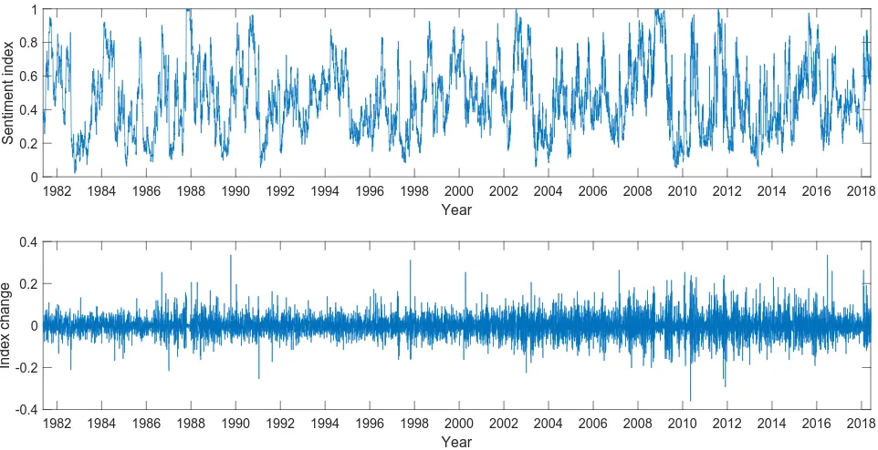
two cases, we consider the dynamics of the sentiment index and its evolution over time. Fig. (1) shows the
resulting sentiment index zt for the S&P 500 along with the time series of daily changes, which is calculated
as the difference betweenztandzt−1. We observe swings of sentiment of the market between the two extreme
values,z = 0 andz= 1. Such sentiment index resembles the behaviour of the GBR index. Moreover, a visual
6
Fig. 1:Sentiment index and index change of S&P 500.
1982 1984 1986 1988 1990 1992 1994 1996 1998 2000 2002 2004 2006 2008 2010 2012 2014 2016 2018 Year
0 0.2 0.4 0.6 0.8 1
Sentiment index
1982 1984 1986 1988 1990 1992 1994 1996 1998 2000 2002 2004 2006 2008 2010 2012 2014 2016 2018 Year
-0.4 -0.2 0 0.2 0.4
Index change
inspection of the time series of index changes shows the presence of volatility clusters, a phenomenon shared
with the time series of price returns (Cont,2001). Our simple filtering technique might be useful to characterise
the overall behaviour of investors in the market. Fig. (1) shows a remarkable visual similarity to the time
series generated by the herding model proposed by Kirman (Kirman, 1991;Kirman, 1993), which is inspired
by an entomological experiment on the behaviour of ants. In this paper, we analyse to what extent such visual
similarity can be translated into a quantitative correspondence.
4 Kirman Herding Model
Kirman(1991,1993) has popularised an entomological experiment on the behaviour of an ant colony where the
ants can choose between two identical sources of food near their nest. Surprisingly, at a given instant of time,
most of the ants are in the proximity of a source of food instead of observing an equal allocation of ants between
the two sources, and, even more surprisingly, such majority switches over time between the two sources. This
experimental observation has been explained through a combination of recruitment interactions among ants
and an autonomous switching of individual ants, as a result of its stochastic search for food. In particular, the
pairwise recruiting interaction of two ants, due to the exchange of pheromones to communicate to each other,
can be interpreted as a herding behaviour when one ant decides to follow the another regardless of its own
information on the location of the source of food.
Based on this entomological experiment, Kirman has introduced a simple stochastic model in order to
formalise the herding interaction among ants and to explain the aggregate asymmetric behaviour of the colony
in order to model the switching mechanism among different strategies used by agents to trade an asset.7In line
with a large number of contributions in the agent based finance and based on a visual similarity of the time
series, we apply the ant model of Kirman to formally describe the dynamics of the sentiment index defined in
Eq. (8). This allows us to have a formal model of the function and evolution of the sentiment of investors in a
financial market.
As previously described, the stocks are categorised into two states within the optimism/pessimism
di-chotomy. The formalisation of the Kirman herding model starts assuming that the stochastic population
dy-namics, determined by the aggregate variable nt from Eq. (7) evolves according to the Poisson probabilities
governing the change of one stock from nt at time t to some n′t at time t+∆t0, where n′t = nt ±1. These conditional probabilities are denoted by ρ(n′,t + ∆t
0 | n, t). For sufficiently small time increments ∆t0 the probabilities are linear in the time interval and are defined as:
ρ(n+ 1, t+∆t0|n, t) = (N−n)(a1+bn)·∆t0,
ρ(n−1, t+∆t0|n, t) =n(a2+b(N−n))·∆t0,
(9)
with the further constraint that:
ρ(n, t+∆t0|n, t) = 1−ρ(n+ 1, t+∆t0|n, t)−ρ(n−1, t+∆t0|n, t). (10)
Moreover, given that the conditional probabilitiesρ(n′,t +∆t
0 | n,t) must be bounded to 1 and must be positive, an upper limit can be computed for the elementary time step, ∆t0:
∆t0≤
2 bN(N+a1
b + a2
b )
. (11)
The probabilities of Eqs. (9) and (10) define a Markov chain that can be more precisely classified within the
class of non-linear one-step processes (Van Kampen, 1992).8 The constants a
1 and a2 account for the change
of state due to idiosyncratic external events while the term proportional to b represents the market pressure.
An individual stock might change its state due to an idiosyncratic external event, for instance new information
affecting the prospects of future cash flows. A new information affects the trading attitude of investors, triggering
their buy or sell signals on that particular stock, which, in turn, might change the current stock price, possibly
modifying its relative position with respect to EMA and eventually its state. The terms a1 and a2 trigger
random switches among states, regardless of the state of the other stocks. Notice, however, that this sensitivity
7
Two main examples of this literature areLux and Marchesi(2000) andAlfarano et al.(2005). The former relates volatility clustering, fat tails and the unit root property of assets to the interaction of chartists, who can be optimistic and pessimistic, and fundamentalists. In fact, chartists change their mood not only due to the price trend but also because of the majority opinion. The latter also shows that fat tails and volatility clustering can be considered as an emergent property of the interaction of traders, whose main contribution relies on the direct estimation of the underlying parameters of their herding model given a closed-form solution for the distribution of returns.
8
to change the state depends on the direction of the transition, given the asymmetry of the two coefficients (a1
anda2). The state of a stock might also change under the market pressure modelled by the dependence of the
probabilities on the overall number of stocks in the opposite state. In other words, with this term we account for
the global coupling among all stocks in a given market, what is captured within the CAPM by the dependence
of the individual stock return on the return of the index. Collective changes of the mood of investors due to
social interactions based on herd behaviour are reflected into the corresponding changes of states of the stocks.
Our sentiment index can be considered, therefore, a devise to detect indirectly the unobservable movement of
the sentiment of investors. The non-linear term in Eq. (9) accounts for the impact that the mutual influence in
the behaviour of traders has on the collective movements of the stocks.
In Alfarano (2006) and Garibaldi and Scalas (2010), the finitary equilibrium distribution of the Markov
chain of Eq. (9) is derived, which turns out to be a Polya distribution. In order to approximate the discrete
stochastic process by a continuous diffusion process (Alfarano et al.,2005,2008,2013;Alfarano and Milakovi´c,
2009), we define the collective behaviour of the whole market with respect to the intensive variablezt.Alfarano
et al.(2005) shows that the Markov chain of Eq. (9) can be approximated by the dynamics of the variablezt
within the framework of the Fokker-Planck equation (FPE),
∂ρ(z, t)
∂t =−
∂
∂z[A(z)p(z, t)] + 1 2
∂2
∂z2[D(z)p(z, t)], (12)
whereA(z) represents the drift term
A(z) =a1−(a1+a2)z, (13)
while the diffusion termD(z) is given by
D(z) = 2b(1−z)z. (14)
The resulting equilibrium distribution, obtained byAlfarano et al.(2005) is
p0(z) = 1 B(ε1, ε2)
zε1−1(1−z)ε2−1, (15)
where
B(ε1, ε2) = Γ(ε1)Γ(ε2) Γ(ε1+ε2)
, (16)
beingΓ(·) the Gamma function.9,10Interestingly, it turns out that it depends only on the ratiosε
1=a1/b
andε2=a2/bbut not on the size of the constantsa1, a2 andb. The resulting distribution of Eq. (15) is known
as the Beta distribution which is characterised by being a flexible distribution in a bounded domain.
9
Despite the fact that our sentiment indexztis not a continuous variable given the finite number N of stocks in the system, for simplicity of the calculus we examine the Beta as equilibrium distribution instead of the Polya distribution (Alfarano et al.,2005).
10
Instead of simulating the stochastic process of Eq. (9) at the microscopic level with a single transition at a
time or solving the FPE of Eq. (12) (seeAlfarano,2006), we can also describe the herding mechanism, at the
mesoscopic level, by means of a stochastic equation known in the physics jargon as Langevin equation. This
approach allows to approximate the conditional distribution of the discrete process of Eq. (9) to a Gaussian
distribution. In other words, instead of following the herding dynamics at the microscopic time scale∆t0, when
we observe at most a switch of a single asset, we considered a mesoscopic time scale ∆t, during which we
aggregate several variations of the variableztin order to obtain a simpler description of its dynamics.Alfarano
et al. (2005) derive the following approximation for the stochastic process of Eq. (9):
zt+∆t =zt+ (ε1−(ε1+ε2)zt)b∆t+
p
2b∆t(1−zt)zt·λt,
=zt+ (ε1+ε2)(¯z−zt)b∆t+
p
2b∆t(1−zt)zt·λt,
(17)
whereλtis a iid normally distributed random variable and ¯ztis defined asε1/(ε1+ε2), which is the mean of
the process itself. The mesoscopic time scale ∆tis proportional toN2, i.e.∆t∼N2∆t
0.11 The process of Eq.
(17) is characterised by a linear mean reverting component and a heteroskedastic random term, conditional to
the value ofzt. Given the parabolic dependence of the diffusion function, values ofztclose to 0.5 generate higher
fluctuations than when ztis close to the boundaries of its range. This dependences generates heteroskedastic
fluctuations in the time series of ∆zt, which may resemble those illustrated in Fig. 1. Obviously, Eq. (17)
is an approximation for large N of the process in Eq. (9), with the further restriction that the variable zt
cannot be close to the boundaries zt = 0 and zt = 1. In those regions, the continuous approximation is no
longer valid since it may violate the boundaries. Hence, the natural boundaries implemented in Eq. (9) must
be exogenously added to Eq. (17). Consequently, in order to simulate the process of Eq. (17), we have to add
reflecting boundaries at zt= 0 andzt= 1 by hand:
if zt>1 then
zt+∆t+zt
2 = 1,
if zt<0 then
zt+∆t+zt
2 = 0,
(18)
which are equivalent to a reflection around the edges of the domain ofzt,zt= 1 andzt= 0, respectively. One
of the advantages of the Langevin equation is that it is relatively simple to estimate via maximum likelihood,
since the conditional probability density function of zt+∆t given zt is a Gaussian with mean zt+ (ε1−(ε1+ ε2)zt)b∆tand standard deviation
p
2b∆t(1−zt)zt.
Finally,Alfarano et al.,2005derive the autocorrelation function (ACF) through the Langevin equation by
using a recursive method12, leading to an exponential autocorrelation function:
Cz(t) =e−b(ε1+ε2)t. (19)
11
SeeAlfarano et al.(2008) for the details of the derivation. 12
Summarising, the model of Eq. (17) is characterised by a Beta equilibrium distribution, a mean reverting
property with heteroskedastic persistent fluctuations and an exponential autocorrelation function. Moreover, a
crucial chracteristic of the model is that can be easily estimated using the maximum likelihood estimator.
5 Validation of the model and estimation of its parameters
We compare the empirical properties of the sentiment index from Eq. (8) to the theoretical properties of the
index as described in the previous section. In particular we confront the unconditional distribution of the
index zt, the time series of daily changes and the autocorrelation function. The sentiment index,zt, computed
based on the 208 stocks that have been present in the stock market from 01/01/1981 to 01/06/2018, while the
simulated sentiment index, zs
t, has been computed by using the Langevin equation (Eq. (17)) with estimated
parameters from empirical data. First and foremost, we estimate the three parameters which characterise the
model by means of the Langevin equation as an aggregate law of motion using the maximum likelihood method.
Alternatively, we estimate the parametersε1andε2using the maximum likelihood method but with a likelihood
based on the unconditional distribution from Eq. (16) (seeAlfarano et al.(2005) for the details of the method).
The parameter b, which governs the time scale of the process, does not enter in the determination of the
unconditional distribution.
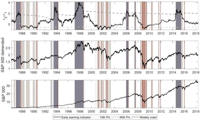
In Table2we show the estimations ofε1,ε2,b, and the corresponding fit of the unconditional distribution
in Fig. (2). We can observe that the parameters estimated using the Beta distribution give rise to a better fit of
the empirical probability density function of the sentiment index than the corresponding parameters estimated
using Eq. (17). We observe, in fact, the presence of a clear asymmetry in the empirical distribution, while the
estimated values point to a symmetric distribution. Such poor performance of the Langevin equation, compared
to the estimation based solely on the unconditional distribution, signals a certain degree of incoherence between
the conditional property of the process in Eq. (17) and the stimated unconditional distribution from the data.
Such discrepancy does not come as a surprise. The Langevin dynamics, in fact, does not constitute a good
approximation of the continuous process of Eq. (12) at the boundaries, and therefore, it cannot be estimated
with the second approach.
Table 2: Estimated parameters,ε1,ε2 andbfor the sentiment index.
Method ε1 ε2 b
Unconditional distribution 1.99±0.07 2.25±0.06
-Langevin equation 1.64±0.16 1.74±0.14 0.0055±0.0001
Given the poor performance of the Langevin, we analyse whether there are a few observations at the
boundaries heavily affecting the estimation of the parameters. We observe that the values ofzt>0.95 are 141
daily events, i.e. 1% of the data at our disposal.
Simulating the stochastic process with the estimated parameters of S&P 500 index (ε1= 1.99 andε2= 2.25)
Fig. 2:Probability density function of the sentiment index compared to the theoretical distribution given the estimates of each method.
0 0.2 0.4 0.6 0.8 1
Empirical sentiment index 0 0.5 1 1.5 2 Density Unconditional distribution Empirical PDF Theoretical PDF
0 0.2 0.4 0.6 0.8 1
Empirical sentiment index 0 0.5 1 1.5 2 Density Langevin equation Empirical PDF Theoretical PDF
Table 3: Estimated parameters,ε1,ε2 andbfor the sentiment index, excluding extreme negative events (zt>0.95).
Method ε1 ε2 b
Unconditional distribution 2.28±0.09 2.72±0.10
-Langevin equation 2.22±0.18 2.86±0.22 0.0054±0.0001
simulated data, we obtain 42.13 In other words, we have observed more than three times extreme events than
theoretically expected. Excluding those events from the estimation we obtain the parameters in Table3and the
fit of the corresponding unconditional distribution in Fig. (3). Both methods improve the fit of the empirical
data. Interestingly, we cannot reject that the estimates from the Langevin and the unconditional distribution
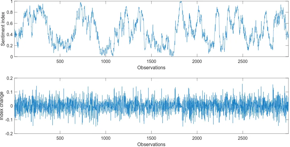
are equal considering the standard error. Fig. (1) and Fig. (4) shows the empirical and simulated index with
their corresponding daily changes. Both time series exhibit swings of pessimism and optimism with visually
similar characteristics. The time series of the empirical changes of the index and the corresponding simulated
time series exhibit heteroskedastic fluctuations. In particular, the higher level of fluctuations is associated to a
value of the sentiment index around an equilibrated population of stocks (zt = 1/2), while the lower level of
fluctuations is concentrated in regions far from zt= 1/2.
Fig. 3:Probability density function of the sentiment index compared to the theoretical distribution given the estimates of each
method and excluding extreme negative events (zt>0.95).
0 0.2 0.4 0.6 0.8 1
Empirical sentiment index 0 0.5 1 1.5 2 Density
Unconditional distribution
Empirical PDF Theoretical PDF
0 0.2 0.4 0.6 0.8 1
Empirical sentiment index 0 0.5 1 1.5 2 Density Langevin equation Empirical PDF Theoretical PDF 13
Fig. 4:Simulated sentiment index and index change with the following parameters:ε1= 1.99,ε2= 2.25,N= 208.
500 1000 1500 2000 2500
Observations 0
0.2 0.4 0.6 0.8 1
Sentiment index
500 1000 1500 2000 2500
Observations -0.2
-0.1 0 0.1 0.2
[image:14.595.59.539.78.322.2]Index change
Fig. 5:Autocorrelation function of the sentiment index compared to the theoretical autocorrelation function.
0 10 20 30 40 50 60 70 80 90 100
Lag -0.2
0 0.2 0.4 0.6 0.8
1 Autocorrelation function
Theoretical decay Empirical decay
0 10 20 30 40 50 60 70 80 90 100
Lag -2.5
-2 -1.5 -1 -0.5
0 Autocorrelation function (log)
Theoretical decay Empirical decay
Once we have analysed the goodness of fit of the unconditional properties of the model in describing the
distribution of the sentiment index and its changes, we focus our attention on the time series properties.
In order to do so, we consider the autocorrelation function. Fig. (5) shows the fit of the autocorrelation of
the empirical distribution as compared to the theoretical autocorrelation function from Eq. (19), which turns
out to be particularly accurate. We can conclude that the calibrated herding model can satisfactorily describe
the degree of persistence of the time series of the sentiment indexzt.
6 Empirical application: Early warning indicator
The sentiment of investors in financial markets has been analysed from many different approaches in a sizeable
examples are the Index Cohesive Force (Kenett et al.,2011;Kenett et al.,2012), power law distributions (Kaizoji,
2006; Mizuno et al., 2016), the leverage of the banking sector (Adrian and Shin, 2009), cross-correlations
(Podobnik et al., 2009), CAPE ratio (Shiller, 2015) and regime switching approaches (Preis et al., 2011),
among other studies. We aim now to employ the sentiment index developed in the previous sections to detect
potential optimistic phases in the market, with the objective of providing an early warning indicator of possible
downturn periods.
The dynamics of the variable zt itself is too volatile to be employed as a direct measure of the phase of
the market, as we can see from Fig. (1). We have, then, to find a meaningful filtering technique in order
to extract a more readable signal from the raw time series of the sentiment index zt. In order to aggregate
the information of the sentiment index during a given time interval and identify the phase of the market, we
estimate the parameters ε1,t and ε2,t through a rolling window of 750 days (three years). We implement a
recursive estimation for ε1,tandε2,t using the observations ofztfromt−750 tot. Under the assumption that the Eq. (17) is the law of motion of the sentiment index, we estimate the parametersε1,t,ε2,tandbtusing the
maximum likelihood method for each rolling window.14 Given that the relaxation time scale15of the process of
Eq. (17) isτc = 1/[(b(ε1+ε2)]≈20 days, we can reasonably assume that the Beta distribution with parameters ε1,t and ε2,t is a good approximation of the unconditional distribution of the process within a given rolling
window. We can, then, employ some characteristics of the Beta distribution as a summary indicator for the
phase of the market. In particular, we identify in a measure of the asymmetry of the Beta distribution a proper
summary indicator. As a measure of asymmetry, we use the difference between the value of the two estimated
parameters16:
Λt=ε2,t−ε1,t. (20)
We contemplate three different scenarios:ε2,t≈ε1,t, so thatΛt≈0, which represents a “symmetric” market with approximately the same number of stocks in a pessimistic and optimistic phase; ε2,t > ε1,t and Λt >0
represent a bull market, when most of the stock prices are, on average, raising at the same time; finallyε2,t< ε1,t
and Λt < 0 underline the existence of a bear market, when most of the stock prices are, on average, falling
simultaneously (see Fig. (6)).
Fig. (7) shows the evolution of the indicatorΛtusing a 100-day EMA and a time interval of 750 days for the
estimation of parameters. To obtain a sharper characterisation of the phase of the market, we consider certain
levels of “excess asymmetry”, establishing a threshold equal to 90th percentile, which is represented by dark
grey areas, for bull phases, and a threshold equal to 10thpercentile, which is represented by light grey areas, for
14
We use all data in each window without removing extreme values. In this case, using short running windows, we do not observe that extreme events affect the fit of the distribution. In fact, we observe similar results even excluding those values ofzt>0.95.
15
The characteristic time scaleτccan be derived considering the autocorrelation function from Eq. (19). 16
Fig. 6:Three possible scenarios for the stock index based onε1andε2. In the first one (ε1 < ε2), there is optimism in the market. In the second one (ε1≈ε2), there is no dominant mood. In the last one (ε1> ε2), there is pessimism in the market.
0 0.2 0.4 0.6 0.8 1
0 1 2 3
Density
0 0.2 0.4 0.6 0.8 1
0 1 2 3
Density
0 0.2 0.4 0.6 0.8 1
0 1 2 3
Density
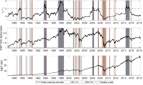
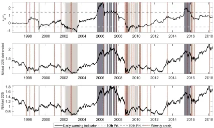
Fig. 7:Early warning indicator using 100-day EMA and a time interval of 750 days for the estimation of parameters. Light
and dark grey areas represent the 10th(bear market) and 90th(bull market) percentiles. Dotted red line denotes the 30 most negative weekly returns. S&P 500 index.
Note. Bull market phases and the subsequent negative events: 1987 (black monday), 1994 (tightening monetary policy), 1997-1998 (Russian financial crisis), 2006 (tightening monetary policy), 2007 (sub-prime mortgage crisis) and 2015-2016 (weakness of China economy). Bear market phases: 1987-1990 (black monday and Gulf war), 2001-2003 (burst of the dot com bubble), 2008-2009 (burst of the housing bubble).
bear markets.17 Moreover, we plot in Fig. (7) the sequence of the 30 most negative weeks in S&P 500 history.
We additionally show the sequence of the S&P 500 index and its de-trended series.18
17
We compute the two thresholds using the entire data set at our disposal. However, as can be observed in the Appendix, we obtain very similar results using past data to compute recursively the value of the two thresholds.
18
Given that we are not analysing exactly S&P 500, since we only have 208 stocks at our disposal, we show the corresponding index of the available stocks ( ¯St), defined as the exponential cumulative sum of market returns at each time t,
¯
St=emrt·t, (21)
wheremrtdenotes the market return at t defined as:
mrt= 1 N
N
X
i=1
ri,t, N= 208, (22)
Fig. (7) shows the different periods in which we observe the sequence of optimistic and pessimistic phases
of the market, along with extreme negative weekly events. The objective of this figure is to evaluate the
performance of the early warning indicator with empirical data, that is:
– we expect to observe at least a down-trend period (underlined by negative weeks in the stock index) shortly
after the early warning indicator has detected a bull market phase (around its 90thpercentile).
As a second hypothesis:
– we expect higher prices after bear market phases (around its 10thpercentile) due to the low prices of stocks
during extreme pessimistic phases.
Therefore, the detection of the bull and the bear market phases can be exploited by investors to set a
long-term trading strategy based on the prospect of future prices. In particular, a possible trading strategy
detecting a bull market phase would be based on the progressive sale of stocks, or the purchase of put-options,
in order to avoid the down-trends or persistent downturns. In the opposite scenario, a bear market would give
the opportunity to accumulate stocks due to the low stock prices as a consequence of the pessimism in the
market. The early warning indicator can be also considered as a valid instrument for policy-makers to set more
efficient policies in order to avoid the contagion from the financial side to the real side of the economy.
In Fig. (7) we identify the following optimistic market phases: 1987, 1994, 1997-1998, 2006, 2007 and
2014-2015. In favour of the proper performance of the indicator, all these optimistic phases of the market precede at
least an extreme negative weekly return, which are triggered by well-identified events. In chronological order,
the first optimistic period appears some months before the black monday (October, 1987), from April to August
1987. In fact, we observe in our sample the most negative event with a weekly return equal to -18.92% due to
the errors of the computerised trading system, which triggered sell orders of an enormous block of stocks as
prices fell (Waldrop,1987). The second optimistic period is detected from March 1997 to August 1998, whose
end is found on the last week of August 1998 as a result of the Russian financial crisis (Buchs, 1999) with
a negative weekly return of -7%. Another extreme optimistic period in the S&P 500 can be identified, from
January to May 2006, in which a down-trend stopped the increase in prices due to a new prospect of further
tightening of the monetary policy in USA, Europe and Japan (IMF,2006). Despite this small decrease in prices,
the optimism remained in the market with another peak of optimism from June to July 2007. Interestingly,
our indicator includes the maximum price previously to the United States bear market (2007-2009), triggered
by the subprime mortgage crisis in October 2007 (Demyanyk and Van Hemert, 2009). The last optimistic
period observed in our sample is detected during 2014-2015, which arise from the unconventional expansionary
monetary policy implemented by the central banks, known as quantitative easing, generating an increase in
prices without precedence that still remains nowadays. This surprising scenario has only been interrupted by
the stock market sell-off in 2015, as a result of fears about China economy and investors concerns over the end
of the quantitative easing (Bendini,2015; Sornette et al.,2015). Our empirical analysis stresses the validity of
the early warning indicator since the six extreme bull market phases identified by the early warning indicator
Focusing on the second hypothesis, Fig. (7) shows generally three extreme pessimistic periods (levels around
the 10thpercentile): after the black monday (1987-1990), the burst of the Dot com bubble (2001-2003) and the
burst of the housing bubble (2008-2009). As can be observed from the S&P 500 index, there is a considerable
increase in prices after the detection of the pessimistic phase. In particular, we can mention three increases
in prices: after the Gulf war (1990), after the burst of the dot com bubble (2003), and after the burst of the
housing bubble (2005). Thus, the persistent downturns can be used to progressively accumulate call-options or
stocks since it is expected the end of the pessimistic phase of the market.
7 Robustness analysis
So far, we have examined the statistical properties of our proxy for the mood of investors estimated using the
collective movement of S&P 500 stocks. However, any stock market can be potentially driven in some measure
by agent’s sentiment. Different statistical properties of the evolution of the sentiment index could characterise
diverse stock markets due to factors like country’s features (Anderson et al.,2011,Karlsson and Nord´en,2007)
proportion of institutional investors, firm size (Ferreira and Matos,2008) or reports quality (Biddle et al.,2009)
among other aspects. Given these differences among markets, it is interesting to study whether the sentiment
index and the early warning indicator can be meaningfully applied to other financial markets regardless of the
evident differences among countries and indexes.
In order to do so, we repeat the procedure to compute the sentiment index for two alternative data sets: US
stock markets and worldwide stock markets. On the one hand, examining different stock markets in the same
country, i.e. assuming that the country features are invariant, we study whether aspects like firm size, proportion
of institutional investors, liquidity or the specificity of a sector can affect the behaviour of the sentiment index.
We analyse, therefore, the S&P 400 midcap index whose companies are smaller than S&P 500 firms, with a
lower level of liquidity and a clear different proportion of institutional investors given the absence of analyst
recommendations for these companies. We also analyse the Nasdaq index, whose core business of the companies
is focused on the information technology sector.
On the other hand, we study the indexes of 6 different countries in order to observe whether a different result
arises, not only due to stock market characteristics but also due to country features like culture or economic
conditions. Thus, we examine the following countries and indexes: ASX 200 (Australia), TSX (Canada), Euro
Stoxx 600 (Europe), Nikkei 225 (Japan), JSE (South Africa) and FTSE 100 (UK).
7.1 US stock markets
Investor preference is one of the main features to take into account in order to know who is investing in each type
of market. In fact,Ferreira and Matos(2008) show that institutional investors prefer firms that are characterised
by being large, well-governed and with high levels of stock-trading liquidity. In the same line,Aggarwal et al.
Table 4: Estimated parameters,ε1,ε2 andbfor U.S. stock indices. The Langevin equation has been used to obtain the esti-mates excluding extreme negative events (zt>0.95).
Stock market Date ε1 ε2 b
S&P 400 midcap 1993-2018 2.55±0.23 2.72±0.23 0.0060±0.0002
Nasdaq 1993-2018 2.18±0.17 2.82±0.21 0.0088±0.0002
Fig. 8:Probability density function of the U.S. sentiment indices compared to the theoretical distribution. The Langevin
equa-tion has been used to obtain the estimates excluding extreme negative events (zt>0.95).
0 0.2 0.4 0.6 0.8 1
Empirical sentiment index 0
0.5 1 1.5 2 2.5
Density
S&P400 midcap
Empirical PDF Theoretical PDF
0 0.2 0.4 0.6 0.8 1
Empirical sentiment index 0
0.5 1 1.5 2 2.5
Density
Nasdaq 100
Empirical PDF Theoretical PDF
The relevance of financial reports is highlighted by Biddle et al.(2009) since those firms with higher financial
reporting quality suffer less from macro-economic conditions and deviate less from predicted investment levels.
Financial aspects are also crucial since domestic managers prefer companies with large dividends, low financial
distress and low return variability (Covrig et al., 2006), which are features of firms with high market
capitali-sation. Considering these characteristics, institutional investors would prefer to invest in companies from S&P
500 rather than those from S&P 400 midcap. If we consider the median total market cap, S&P 500 is 5 times
larger than S&P 400 midcap, with the following market capitalisation: 20493.91 and 4178.83 US millions for
S&P 500 and S&P 400 respectively.19
Despite differences among these indexes it is possible to observe in Fig. (8) and Table4that the estimates are
in line with those obtained for the S&P 500. Moreover, if we use stock markets like Nasdaq, focused on firms from
the information technology sector, we keep observing very similar estimates. Therefore, even with a different
type of investor, liquidity, sector, or market cap, our proxy for the sentiment of investors shows very similar
statistical properties: volatility clustering in the time series of sentiment index increments and the exponential
autocorrelation function of the sentiment index (the statistical analysis is shown in the supplementary material).
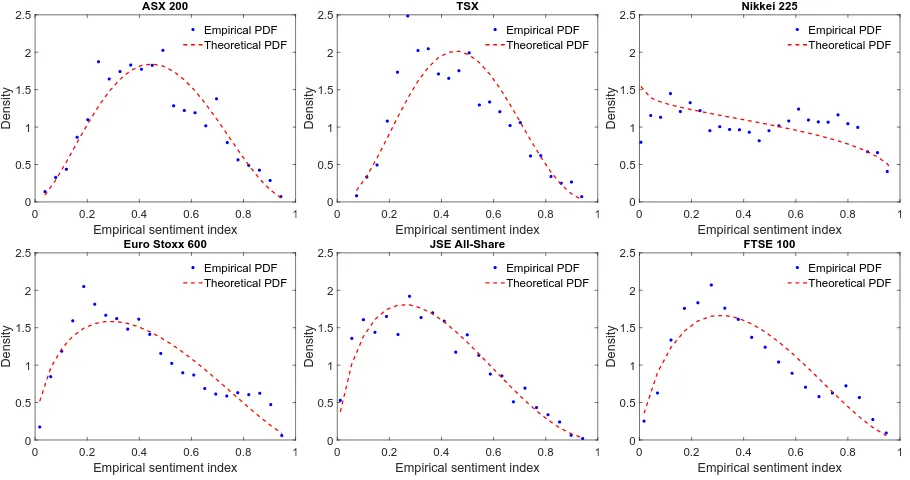
7.2 Worldwide stock markets
A remarkable feature of worldwide stock markets is the high level of portfolio concentration in domestic markets.
This phenomena, known as “home bias”, goes not only against the advantages of international diversification
but also many standard asset-pricing models. This traditional feature, which was highlighted in the 90s by
French and Poterba(1991),Cooper and Kaplanis(1994) andTesar and Werner(1995), is still present nowadays
19
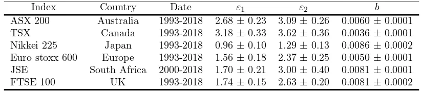
Table 5: Estimated parameters,ε1,ε2 andbfor worldwide stock indices. The Langevin equation has been used to obtain the estimates excluding extreme negative events whenzt>0.95.
Index Country Date ε1 ε2 b
ASX 200 Australia 1993-2018 2.68±0.23 3.09±0.26 0.0060±0.0001
TSX Canada 1993-2018 3.18±0.33 3.62±0.36 0.0036±0.0001
Nikkei 225 Japan 1993-2018 0.96±0.10 1.29±0.13 0.0086±0.0002
Euro stoxx 600 Europe 1993-2018 1.56±0.18 2.37±0.25 0.0050±0.0001
JSE South Africa 2000-2018 1.70±0.21 3.00±0.40 0.0081±0.0001
FTSE 100 UK 1993-2018 1.74±0.15 2.63±0.20 0.0081±0.0002
despite the many improvements in terms of information channels.20 Anderson et al. (2011) demonstrate that
home bias exists in institutionally managed portfolios from more than 60 countries. In the same vein,Grinblatt
and Keloharju (2001) with a database focused on Finland, contend that investors prefer those firms that are
nearby with a common language and culture.
In this line, home bias underlines the fact that local agents are investing in those companies and stocks
that are present in the corresponding local or domestic financial market. Therefore, we can assume that when
analysing a worldwide stock market, the main proportion of capital is given by local investors. This aspect is of
paramount importance for this study since the fact of observing a proper fit of the unconditional distribution
of the sentiment index, regardless of the country, implies that we can use our model to describe optimism
and pessimism of agents regardless of the country specific characteristics. Table 5 and Fig. (9) show how the
Langevin process provides us with a fairly homogeneous description of financial markets from different countries.
The estimated parameters are in fact fluctuacting in a narrow range of variability. Excluding the Nikkei 225
index, the sentiment index of all the other financial markets seem to be well characterised by an asymmetric
uni-modal Beta distribution, with non-monotonic probability density. Also in the case of international markets,
we observe heteroskedastic fluctuations of the index increments and an exponential decay of its autocorrelation
(the results in the supplementary material).
7.3 Global financial village
The fact that all the financial markets have become a coupled complex system is not surprising given the
correlation between stock market indices (Mantegna and Stanley, 1996; Forbes and Rigobon, 2002), as it is
underlined by Kenett et al. (2012) when identifying that U.S., U.K., Germany and Japan indices are highly
interconnected. Consequently, the “global financial village is highly prone to systemic collapses which can sweep
the entire village” (Kenett et al., 2012). In the same line, by means of our early warning indicator we observe
how all the stock indices are behaving in a similar manner regardless of the country specific characteristics of
each index. The effect of the Russian financial crisis in 1998, the dot com crash in 2001-2003, the burst of the
housing bubble in 2008-2009 and the down-trend in prices during 2015-2016, due to the weakness of China
economy, are the best example of the consequences of the “global financial village”, since, to a greater or lesser
20
Fig. 9:Probability density function of the worldwide sentiment indices compared to the theoretical distribution. The Langevin equation has been used to obtain the estimates excluding extreme negative events (zt>0.95).
0 0.2 0.4 0.6 0.8 1
Empirical sentiment index 0 0.5 1 1.5 2 2.5 Density ASX 200 Empirical PDF Theoretical PDF
0 0.2 0.4 0.6 0.8 1
Empirical sentiment index 0 0.5 1 1.5 2 2.5 Density TSX Empirical PDF Theoretical PDF
0 0.2 0.4 0.6 0.8 1
Empirical sentiment index 0 0.5 1 1.5 2 2.5 Density Nikkei 225 Empirical PDF Theoretical PDF
0 0.2 0.4 0.6 0.8 1
Empirical sentiment index 0 0.5 1 1.5 2 2.5 Density
Euro Stoxx 600
Empirical PDF Theoretical PDF
0 0.2 0.4 0.6 0.8 1
Empirical sentiment index 0 0.5 1 1.5 2 2.5 Density JSE All-Share Empirical PDF Theoretical PDF
0 0.2 0.4 0.6 0.8 1
Empirical sentiment index 0 0.5 1 1.5 2 2.5 Density FTSE 100 Empirical PDF Theoretical PDF
extent, it is possible to observe those events regardless of the market (see in this section: Nasdaq 100 (U.S.),
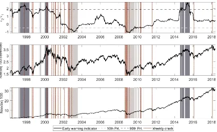
Fig. (10); Eurostoxx 600 (Europe), Fig. (11) and Nikkei 225 (Japan), Fig. (12)).21 As a result, in favour of
the two hypotheses of our early warning indicator, we can identify negative weekly returns after an optimistic
market phase has been detected, while a pessimistic market phase is characterised by low prices compared to
the future price of the indices. In fact, we identify a high concentration of negative weekly returns in all the
stock indices after the burst of the housing bubble (2008-2009), along with a lower concentration during the
burst of the dot com bubble (2001-2003), and the down-trend caused by China economy (2015-2016).
However, despite the fact that all the stocks indices are generally affected by similar negative events, it
is interesting to observe that a bubble originated in one specific market is generating financial downturns in
other markets that were not involved in such optimistic scenario. To explain this point, we underline two main
periods of the recent financial history (the dot com bubble and housing bubble) using the main stock indices
(S&P 500 (U.S.), Fig. (7); Nasdaq 100 (U.S.), Fig. (10); Eurostoxx 600 (Europe), Fig. (11) and Nikkei 225
(Japan), Fig. (12)). As can be easily observed, despite the Russian financial crisis in 1998, investors trading in
Nasdaq stocks maintained their positive mood giving rise to a bull market from February to May 2000. The
burst of the bubble was in March 2000, as we can note due to the continuous negative weeks in Fig. (10).
21
Fig. 10: Early warning indicator using 100-day MA and a time interval of 750 days for the estimation of parameters. Light and dark grey areas represent the 10th(bear market) and 90th(bull market) percentiles. Dotted red line denotes the 30 most nega-tive weekly returns. Nasdaq 100 index.
Note. Bull market phases and the subsequent negative events: 1997-1998 (Russian financial crisis), 2000 (burst of the dot com bubble) and 2015-2016 (weakness of China economy). Bear market phases: 2002-2003 (burst of the dot com bubble) and 2008-2010 (burst of the housing bubble).
Fig. 11: Early warning indicator using 100-day MA and a time interval of 750 days for the estimation of parameters. Light and
dark grey areas represent the 10th(bear market) and 90th(bull market) percentiles. Dotted red line denotes the 30 most nega-tive weekly returns. Euro stoxx 600 index.
[image:22.595.86.512.480.736.2]Fig. 12: Early warning indicator using 100-day MA and a time interval of 750 days for the estimation of parameters. Light and dark grey areas represent the 10th(bear market) and 90th(bull market) percentiles. Dotted red line denotes the 30 most nega-tive weekly returns. Nikkei 225 index.
Note. Bull market phases and the subsequent negative events: 2006 (tightening monetary policy), 2007 (subprime mortgage crisis) and 2015-2016 (weakness of China economy). Bear market phases: 2002-2003 (burst of the dot com bubble) and 2008-2010 (burst of the housing bubble).
Surprisingly, we do not observe the previous optimism to the burst in the rest of indices, like S&P 500 or
Euro Stoxx 600. In fact, Nikkei 225 does not even have an optimistic period before the Russian financial crisis.
However all the markets suffered from the burst of the dot com bubble with a wave of pessimism during the
following years, mainly, from 2001. In other words, the bubble originated in a particular market (Nasdaq) due to
the optimism of their traders, and the resulting herding phenomena, gave rise to a pessimistic scenario in very
different markets (S&P 500, Eurostoxx 600, Nikkei 225, and the rest of the markets in the Appendix) whose
traders were not so optimistic. Interestingly, we can observe during the housing bubble the opposite scenario.
A wave of optimism dominates most of the stock markets like the Eurostoxx 600 and Nikkei 225 indices, which
are affected by the same negative events in May 2006 and October 2008 as in the S&P 500 index. Nevertheless,
Nasdaq 100 does not have an optimistic period nor it is affected by the same negative events during this period.
At any rate, and in the same line as the dot com bubble, Nasdaq and all the markets suffered from the housing
crash, even though there is not an optimistic phase in the Nasdaq index, i.e. despite the fact that there is
not a bubble in a specific market, this market will be affected by the mood of other markets due to financial
contagion. Therefore, the early warning indicator also allows us to describe the different behaviour of each stock
index in a more detail level, even though all of them are connected, as can be observed due to the effect of the
8 Conclusion
Inspired by the Bank of America Merrill Lynch Global Breath Rule, we have introduced an index of financial
investor sentiment based on the collective movements of the stocks in a given financial market. The underlying
hypothesis is that such index reflects and captures the collective behaviour of the investors influencing each
other in waves of optimism and pessimism transmitted by the social interactions. The indexztaggregates the
state of each single stock, which depends on the relative position of its price with respect to the 100-day EMA.
The time evolution of the index can be successfully described by the herding model introduced byKirman(1991,
1993). In particular, the unconditional distribution of the sentiment index, the heteroskedastic fluctuations of
the time series of its increments and the autocorrelation function match the analytical properties of the herding
model. Based on the herding model and the sentiment index, we introduce an early warning indicator, using the
distributional asymmetry of the sentiment index computed in a rolling window. Our early warning indicator
can clearly identify the optimistic and pessimistic phases of the market. Thus, investors can devise strategies to
effectively exploit the early warning indicator. Our results are robust when applying the early warning indicator
to other indices of the US financial markets or financial market indices of other countries like Japan, Australia
or Canada among others.
Acknowledgements
The authors are grateful for funding the Universitat Jaume I under the project P11B2015-63, the Generalitat
Valenciana under the project AICO/2018/036 and the Spanish Ministry Science and Technology under the
project ECO2015-68469-R. The first author acknowledges financial support of Spanish Ministry of Education
(grant number FPU2015/01434) and is thankful to Department of Management of the Universit`a Politechnica
delle Marche for its hospitality during the early stage of this investigation.
9 Appendix
9.1 A1: Robustness analysis of the determination of the thresholds
In order to study the robustness of the results of Fig. (7), we compute the two thresholds at 10th and 90th
percentile using past data instead of the entire sample. So, we compute the percentiles considering (i) 500 data
points, from day 1 to day 500; (ii) adding the other values of Λt, from 501 to the end of the time series and
computing the new values of the thresholds. As we can see from Fig. (13), the results are essentially unchanged
with respect to Fig. (7). This exercise shows that we can use the current value of the thresholds to make
Fig. 13: Early warning indicator using 100-day MA and a time interval of 750 days for the estimation of parameters. Light and dark grey areas represent the 10th(bear market) and 90th(bull market) percentiles. Dotted red line denotes the 30 most nega-tive weekly returns. S&P 500 index.
Note. Bull market phases and the subsequent negative events: 1987 (black monday), 1994 (tightening monetary policy), 1997-1998 (Russian financial crisis), 2006 (tightening monetary policy), 2007 (subprime mortgage crisis) and 2015-2016 (weakness of China economy). Bear market phases: 1987-1990 (black monday and Gulf war), 2001-2003 (burst of the dot com bubble) and 2008-2009 (burst of the housing bubble).
9.2 A2: Early warning indicator
Fig. 14: Early warning indicator using 100-day MA and a time interval of 750 days for the estimation of parameters. Light and
dark grey areas represent the 10th(bear market) and 90th(bull market) percentiles. Dotted red line denotes the 30 most nega-tive weekly returns. S&P 400 midcap index.
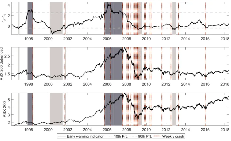
[image:25.595.104.495.498.739.2]Fig. 15: Early warning indicator using 100-day MA and a time interval of 750 days for the estimation of parameters. Light and dark grey areas represent the 10th(bear market) and 90th(bull market) percentiles. Dotted red line denotes the 30 most nega-tive weekly returns. ASX 200 index.
Note. Bull market phases and the subsequent negative events: 1997-1998 (Russian financial crisis), 2006 (tightening monetary policy) and 2007 (subprime mortgage crisis). Bear market phases: 2000-2001 (burst of the dot com bubble) and 2009 (burst of the housing bubble).
Fig. 16: Early warning indicator using 100-day MA and a time interval of 750 days for the estimation of parameters. Light and
dark grey areas represent the 10th(bear market) and 90th(bull market) percentiles. Dotted red line denotes the 30 most nega-tive weekly returns. TSX index.
[image:26.595.104.493.499.737.2]Fig. 17: Early warning indicator using 100-day MA and a time interval of 750 days for the estimation of parameters. Light and dark grey areas represent the 10th(bear market) and 90th(bull market) percentiles. Dotted red line denotes the 30 most nega-tive weekly returns. JSE All-Share index.
Note. Bull market phases and the subsequent negative events: 2006 (tightening monetary policy), 2007 (subprime mortgage cri-sis) and 2014-2015 (weakness of China economy). Bear market phases: 2008-2009 (burst of the housing bubble) and 2016 (China financial crash).
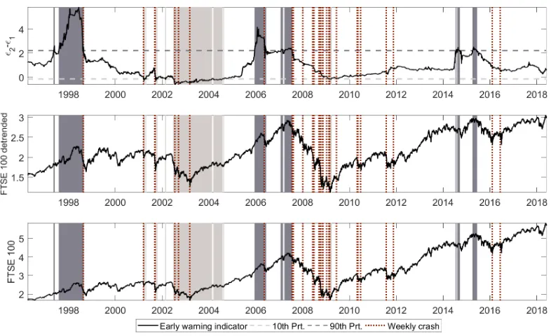
Fig. 18: Early warning indicator using 100-day MA and a time interval of 750 days for the estimation of parameters. Light and
dark grey areas represent the 10th(bear market) and 90th(bull market) percentiles. Dotted red line denotes the 30 most nega-tive weekly returns. FTSE 100 index.
[image:27.595.102.495.499.739.2]References
Adrian, T. and Shin, H. S. (2009). Money, liquidity, and monetary policy. American Economic Review,
99(2):600–605.
Aggarwal, R., Klapper, L., and Wysocki, P. D. (2005). Portfolio preferences of foreign institutional investors.
Journal of Banking & Finance, 29(12):2919–2946.
Alfarano, S. (2006). An agent-based stochastic volatility model. PhD thesis, Christian-Albrechts Universit¨at
Kiel.
Alfarano, S., Lux, T., and Wagner, F. (2005). Estimation of agent-based models: the case of an asymmetric
herding model. Computational Economics, 26(1):19–49.
Alfarano, S., Lux, T., and Wagner, F. (2008). Time variation of higher moments in a financial market with
heterogeneous agents: An analytical approach. Journal of Economic Dynamics and Control, 32(1):101–136.
Alfarano, S., Milakovi´c, M., and Raddant, M. (2013). A note on institutional hierarchy and volatility in financial
markets. The European Journal of Finance, 19(6):449–465.
Alfarano, S. and Milakovi´c, M. (2009). Network structure and n-dependence in agent-based herding models.
Journal of Economic Dynamics and Control, 33(1):78–92.
Anderson, C. W., Fedenia, M., Hirschey, M., and Skiba, H. (2011). Cultural influences on home bias and
international diversification by institutional investors. Journal of Banking & Finance, 35(4):916–934.
Aoki, M. and Yoshikawa, H. (2002). Demand saturation-creation and economic growth. Journal of Economic
Behavior & Organization, 48(2):127–154.
Bendini, R. (2015). Exceptional measures: The shanghai stock market crash and the future of the chinese
econ-omy. Technical report, Policy Department, Directorate General for External Policies, European Parliament’.
Biddle, G. C., Hilary, G., and Verdi, R. S. (2009). How does financial reporting quality relate to investment
efficiency? Journal of accounting and economics, 48(2):112–131.
Black, F. (1986). Noise. The journal of finance, 41(3):528–543.
Buchs, T. D. (1999). Financial crisis in the russian federation: Are the russians learning to tango? Economics
of transition, 7(3):687–715.
Chen, Z. and Lux, T. (2015). Estimation of sentiment effects in financial markets: A simulated method of
moments approach. Computational Economics, pages 1–34.
Cont, R. (2001). Empirical properties of asset returns: stylized facts and statistical issues.
Cooper, I. and Kaplanis, E. (1994). Home bias in equity portfolios, inflation hedging, and international capital
market equilibrium. The Review of Financial Studies, 7(1):45–60.
Covrig, V., Lau, S. T., and Ng, L. (2006). Do domestic and foreign fund managers have similar preferences for
stock characteristics? a cross-country analysis. Journal of International Business Studies, 37(3):407–429.
Demyanyk, Y. and Van Hemert, O. (2009). Understanding the subprime mortgage crisis. The Review of
Financial Studies, 24(6):1848–1880.
Fama, E. F. (1991). Efficient capital markets: Ii. The journal of finance, 46(5):1575–1617.
Feller, W. (1968). An introduction to probability theory and its applications, volume 1. Wiley, New York.
Ferreira, M. A. and Matos, P. (2008). The colors of investors’ money: The role of institutional investors around
the world. Journal of Financial Economics, 88(3):499–533.
Forbes, K. J. and Rigobon, R. (2002). No contagion, only interdependence: measuring stock market
comove-ments. The journal of Finance, 57(5):2223–2261.
Franke, R. and Westerhoff, F. (2011). Estimation of a structural stochastic volatility model of asset pricing.
Computational Economics, 38(1):53–83.
French, K. R. and Poterba, J. M. (1991). Investor diversification and international equity markets. Technical
report, National Bureau of Economic Research.
Friedman, M. (1953). Essays in positive economics. University of Chicago Press.
Garibaldi, U. and Scalas, E. (2010). Finitary probabilistic methods in econophysics. Cambridge University
Press.
Gehrig, T. (1993). An information based explanation of the domestic bias in international equity investment.
The Scandinavian Journal of Economics, pages 97–109.
Gilli, M. and Winker, P. (2003). A global optimization heuristic for estimating agent based models.
Computa-tional Statistics & Data Analysis, 42(3):299–312.
Grinblatt, M. and Keloharju, M. (2001). How distance, language, and culture influence stockholdings and
trades. The Journal of Finance, 56(3):1053–1073.
Hartnett, M., Leung, B., and Roche, G. (2015). Rules & tools: Three buy signals and a funeral. Technical
report, Bank of America Merrill Lynch.
IMF (2006). Global markets analysis division: Financial market update. Technical report, International
Mon-etary Fund.
Ivkovi´c, Z. and Weisbenner, S. (2005). Local does as local is: Information content of the geography of individual
investors’ common stock investments. The Journal of Finance, 60(1):267–306.
Kaizoji, T. (2006). A precursor of market crashes: Empirical laws of japan’s internet bubble. The European
Physical Journal B-Condensed Matter and Complex Systems, 50(1-2):123–127.
Karlsson, A. and Nord´en, L. (2007). Home sweet home: Home bias and international diversification among
individual investors. Journal of Banking & Finance, 31(2):317–333.
Kenett, D. Y., Raddant, M., Lux, T., and Ben-Jacob, E. (2012). Evolvement of uniformity and volatility in the
stressed global financial village. PloS one, 7(2):e31144.
Kenett, D. Y., Shapira, Y., Madi, A., Bransburg-Zabary, S., Gur-Gershgoren, G., and Ben-Jacob, E. (2011).
Index cohesive force analysis reveals that the us market became prone to systemic collapses since 2002. PLoS
one, 6(4):e19378.
Kirman, A. (1991). Epidemics of opinion and speculative bubbles in financial markets. Money and financial