Munich Personal RePEc Archive
A sequential panel selection approach to
cointegration analysis: An application to
Wagner’s law for South African
provincial data
Vayi, Xolisa and Phiri, Andrew
13 September 2018
Online at
https://mpra.ub.uni-muenchen.de/88989/
A SEQUENTIAL PANEL SELECTION APPROACH TO COINTEGRATION
ANALYSIS: AN APPLICATION TO WAGNER’S LAW FOR SOUTH AFRICAN
PROVINCIAL DATA
Xolisa Vayi
Department of Economics, Faculty of Business and Economic Studies, Nelson Mandela
University, Port Elizabeth, South Africa, 6031.
And
Andrew Phiri
Department of Economics, Faculty of Business and Economic Studies, Nelson Mandela
University, Port Elizabeth, South Africa, 6031.
ABSTRACT: This study extends the recently introduced sequential panel selection method
(SPSM) to a cointegration framework which is particularly used to investigate Wagner’s law for 9 South African provinces between 2001 and 2016. We note that when applying single
country/region estimates we fail to find evidence of cointegration whereas within panel
regressions, cointegration effects are present for the entire dataset. In further applying the
SPSM we observed significant Wagner’s effects for panels inclusive of Gauteng, Eastern
Cape and Kwazulu-Natal provinces and when these provinces are excluded from the panels,
cointegration effects are unobserved.
Keywords: Sequential Panel selection method (SPSM); cointegration; Wagner’s law; Provincial analysis; South Africa.
1. INTRODUCTION
There exists an upheld tradition in the econometrics literature of combining
cross-section and time series techniques in investigating numerous important macroeconomic
relationships (see Maddala, 1987 for discussion). One notable fallacy with these ‘panel’ time series econometric models is their generalization of a single regression estimate for a host of
countries or regions which are characterized by multidimensional differences. Recently
Chortareas and Kapetanois (2011) propose the sequential panel selection method (SPSM)
which integrates the size power advantages of panel estimates with the heterogeneity
advantages associated with individual sample estimates. Nevertheless, we note that
Chortareas and Kapetanois (2009) strictly apply the SPSM to unit root procedures in their
empirical investigations. Similarly, studies which have subsequently applied the SPSM
approach have monotonously done so for unit root purposes (see Li et al (2014), Lee (2014)
and Chang et al. (2015) and Anyikwa et al. (2018)).
In our study we extend the SPSM approach to the case of a cointegration regression
analysis. AS far as we are concerned our study becomes the first in the literature to
implement this method. For demonstration purposes we make an application to Wagner’s law for 9 South African provinces. We consider this task relevant since available data on
government expenditure and economic growth for South African provinces is limited to
annual data spanning from 2001 to 2016. Secondly, a number of previous works have studied
this relationship from an aggregated country perspective (Ansari et al. (1997), Ziramba
(2008), Ogbonna (2009), Menyah and Wolde-Rufael (2012), Chipaumire et al. (2014) and
Odhiambo (2015)) hence ignoring the possible differences existing within provincial budgets.
And with the economy struggling to recuperate from the repercussions of the 2009-2010
global recession period, much emphasis has been put on fiscal policy as a vital catalyst for
economic recovery.
The rest of our study is arranged a follows. Section 2 presents an overview of
methodology of the study, section 4 the data and empirical findings whilst the study is
concluded in section 5 of the paper.
2. AN OVERVIEW OF GOVERNMENT SPENDING AND GROWTH IN SOUTH AFRICA
In South Africa, it is stated by the law (in the Constitution) that taxation and
government expenditure be the drivers of budgetary policies (Calitz et al. 2014). The
government has a legal obligation to formulate a fiscal policy that provides and maintains
public funding. Otherwise, failure to comply with this obligation is deemed unconstitutional
(Calitz et al. 2014). This is clearly illustrated in the Bill of Rights of South Africa where each
citizen has the right to basic services such as housing, healthcare, food, water, social security,
and education. Policymakers in South Africa, especially those in government are tasked with
the act of balancing limited resources with unlimited needs. The South African government
has had to invest tremendously in bridging the gap that exists in different regions, developing
social responsibility projects that support and sustain communities, and most importantly
creating and investing in capital infrastructure that is growth promoting.
After the 1994 elections, there was a huge shift in public expenditure and the new
democratic government had to cater to millions under limited resources. Over the last couple
of decades or the democratic ANC government has implemented a number of large scale
expenditure programmes (i.e. the Reconstruction and Development Programme (RDP),
Growth, Employment and Redistribution (GEAR), Accelerated and Shared Growth Initiative
for South African (ASGISA), the National Development Plan (NDP) and the New Growth
Path (NGP) aimed at addressing the social imbalance inherited from the former Apartheid
regime. The national budget has being the most common tool for income redistribution which
to no surprise, led to fiscal deficits (Phiri. 2017) and in 2012, current expenditure, social
benefits paid and services on public debt accounted for 92.3 percent of general government
expenditure. Overall, with the size and composition of the public sector in South Africa have
2012), it is quite surprising that this has not been mirrored onto improved economic growth
rates for the country.
From an academic standpoint, the empirical evidence on Wagner’s law for South
Africa is far from reaching a consensus. Whilst the previous studies of Ogbonna (2009),
Menyah and Wolde-Rufael (2012), Odhiambo (2015) and Phiri (2017) validate Wagner’s effect, in which a larger government size is accompanied with increased economic growth, on
the other hand, the works of Ansari et al. (1997), Ziramba (2008) and Chipaumire et al.
(2014) fail to find any significant Wagner effects. We note the ambiguity observed in these
previous findings may be due to the aggregated approach taken by the aforementioned
authors in reaching their various conclusions on Wagner’s law for South Africa. However, as
mentioned by Narayan et al. (2008), the use of provincial data is advantageous towards
investigating Wagners law since provincial data is consistent with the peace and stability
assumption since provincial budgets do not incur military spending items. Moreover, relying
on sub-national data implies the exploitation of cross-sectional dimension while minimizing
the effects of cultural and institutional differences as well as influences of state expenditure in
dealing with changes in the international economic conditions, all which are important
assumption underlying Wagner’s law.
3. EMPIRICAL FRAMEWORK
3.1 Wagner’s specifications
The academic literature indicates the existence of six versions of Okun’s law, namely the (1) Peacock-Wiseman (1961) version; (2) Pryor (1969) version; (3) Goffman (1968)
version; (4) Musgrave version (1969); (5) Gupta version (1967); and (6) Mann (1968)
version. These versions are respectively specified below in regressions (1) to (6) for South
African individual provinces:
C= f(Y) (2)
G = f(Y/P) (3)
G/Y = f(Y/P) (4)
G/P = f(Y/P) (5)
G/Y = f(Y) (6)
Where G stands for real government expenditure, C stands for government
consumption expenditure, Y stands for real GDP, G/Y is share of government spending in
GDP, P is population such that Y/P is per capita GDP, and G/P is government spending per
capita. Using log-linear functional form for each version, where t is the time subscript and e
is the random error term, the following ARDL specifications can be specified for empirical
purposes:
𝑔𝑡 = 0+ 1𝑖 𝑝
𝑖=1 𝑔𝑡−𝑖+ 2𝑖
𝑝
𝑖=1 𝑦𝑡−𝑖 + 1𝑖𝑔𝑡−𝑖 + 2𝑖𝑦𝑡−𝑖 + 𝑡 (7)
𝑐𝑡 = 0 + 1𝑖 𝑝
𝑖=1 𝑐𝑡−𝑖+ 2𝑖
𝑝
𝑖=1 𝑦𝑡−𝑖 + 1𝑖𝑐+ 2𝑖𝑦𝑡−𝑖+ 𝑡 (8)
𝑔𝑡 = 0+ 1𝑖 𝑝
𝑖=1 𝑔𝑡−𝑖+ 2𝑖
𝑝
𝑖=1 𝑦/𝑝𝑡−𝑖 + 1𝑖𝑔𝑡−𝑖 + 2𝑖𝑦/𝑝𝑡−𝑖+ 𝑡 (9)
𝑔/𝑦𝑡= 0+ 1𝑖 𝑝
𝑖=1 𝑔/𝑦𝑡−𝑖 + 2𝑖
𝑝
𝑖=1 𝑦/𝑝𝑡−𝑖 + 1𝑖𝑔/𝑦𝑡−𝑖 + 2𝑖𝑦/𝑝+ 𝑡 (10)
𝑔/𝑝𝑡= 0+ 1𝑖 𝑝
𝑖=1 𝑔/𝑝𝑡−𝑖 + 2𝑖
𝑝
𝑔/𝑝𝑡= 0+ 1𝑖 𝑝
𝑖=1 𝑔𝑝𝑡−𝑖 + 2𝑖
𝑝
𝑖=1 𝑦𝑡−𝑖+ 1𝑖𝑔/𝑝𝑡−𝑖+ 2𝑖𝑦+ 𝑡 (12)
Where the small letter represents the log transformation of the series, is a first
difference operator, 0 is the intercept term, the parameters 1, …, 2 and 1, …, 2 are the
short-run and long-run elasticities, respectively, and t is a well-behaved error term. The
bounds test for cointegration can be implemented straightforward by testing the null
hypothesis of no cointegration (i.e. 1 = 2 = 0), which is tested against the alternative
hypothesis of ARDL cointegration effects (i.e. 1≠ 2 ≠ 0). Only if the F-statistic exceeds the
upper critical bound, then cointegration effects are validated and the following unrestricted
error correction model (UECM) representation of the ARDL regressions (8) can be modelled:
𝑔𝑡 = 0+ 1𝑖 𝑝
𝑖=1 𝑔𝑡−𝑖+ 2𝑖
𝑝
𝑖=1 𝑦𝑡−𝑖 + 𝑒𝑐𝑡𝑡−1+ 𝑡 (13)
𝑐 = 0+ 𝑝 1𝑖
𝑖=1 𝑔𝑐𝑡−𝑖+ 2𝑖
𝑝
𝑖=1 𝑦𝑡−𝑖+ 𝑒𝑐𝑡𝑡−1+ 𝑡 (14)
𝑔𝑡 = 0+ 1𝑖 𝑝
𝑖=1 𝑔𝑡−𝑖+ 2𝑖
𝑝
𝑖=1 𝑦/𝑝𝑡−𝑖 + 𝑒𝑐𝑡𝑡−1+ 𝑡 (15)
𝑔/𝑦𝑡= 0+ 1𝑖 𝑝
𝑖=1 𝑔/𝑦𝑡−𝑖 + 2𝑖
𝑝
𝑖=1 𝑦/𝑝𝑡−𝑖 + 𝑒𝑐𝑡𝑡−1+ 𝑡 (16)
𝑔/𝑝𝑡= 0+ 1𝑖 𝑝
𝑖=1 𝑔/𝑝𝑡−𝑖 + 2𝑖
𝑝
𝑖=1 𝑦/𝑝𝑡−𝑖 + 𝑒𝑐𝑡𝑡−1+ 𝑡 (17)
𝑔/𝑝𝑡= 0+ 1𝑖 𝑝
𝑖=1 𝑔𝑝𝑡−𝑖 + 2𝑖
𝑝
Where ectt-1 is the error correction term, which is measures the speed of adjustment
back to equilibrium subsequent to a shock to the system.
3.2 Sequential panel selection method to cointegration
To conduct the SPSM to cointegration we rely the pooled mean group (PMG) panel
estimation of Pesaran et al. (1999) which is a generalized panel extension of the ARDL
model outlined in the previous section. In it’s generalized form the panel model can be specified as:
𝑌𝑖𝑡 = 0+ 1𝑖𝑋𝑖𝑡+ 2𝑖𝑋𝑖,𝑡−1 + 𝜓𝑖𝑌𝑖,𝑡−1+𝑒𝑖𝑡 (19)
And associated equilibrium error correction representation is given as:
𝑌𝑖𝑡 = 0+ 1𝑖 𝑋𝑖𝑡+ 1𝑖𝑌𝑖,𝑡−1− 0𝑖− 1𝑖𝑋𝑖,𝑡−1+𝑒𝑖𝑡 (20)
Where 0𝑖 = 𝛼𝑖
1− 𝑖, 1𝑖 =
0𝑖+ 1𝑖
1− 𝑖 and i = (ψi- 1). The above described panel cointegration framework is coupled with the panel cointegration test of Kao (1999). In
outlining the Kao (1999) cointegration test, we assume the residual terms obtained from a
panel regression, eit, can be expressed as:
𝑒𝑖𝑡 = 𝑒𝑖𝑡+ 𝑛𝑗=1 𝑗 𝑒𝑖𝑡−𝑗+𝑣𝑖𝑡𝑝 (21)
And from equation (19) the null hypothesis of no cointegration is given as:
H0: = 1 (22)
Kao (1999) suggests that the no cointegration null hypothesis can be tested using the
𝑡𝑘𝑎𝑜 = 𝑡𝑎𝑑𝑓+ 6𝑁 𝑣/(2 𝑜𝑣)
𝑜𝑣
2 /(2
𝑣
2)+3
𝑣
2/(10
𝑜𝑣
2 ) ~ 𝑁(0,1) (23)
Where 𝑡𝑎𝑑𝑓= −1 [ (𝑒𝑖
′𝑄
𝑖𝑒𝑖)]
1 2
𝑁 𝑖=1
𝑠𝑣 . In order to econometrically carry out the SPSM
procedure to cointegration analysis, we firstly produce a series of individual F-statistics, Fi =
(Fj1, Fj2, …, FjM) after carrying out the ARDL bounds test for cointegation on the individual
provinces. We then specify our binary object function, , which takes the value of 1 if the
panel tkao test statistic rejects the null hypothesis of no cointegration and zero otherwise. We
then implement the following 3-stage algorithm to separate the cointegration from
non-cointegrated series.
Stage 1: Initially estimate the PMG regression with all individual provinces included in the
estimation.
Stage 2: Perform a decision rule in which the Kao test statistic given in equation (13)
associated is computed and set = 0 if the test statistic is insignificant or else we set = 1 if
the test statistic is significant. Only if = 1 is true that we continue to the next stage,
otherwise we stop the procedure.
Stage 3: We identify the individual province which produces a β coefficient with the highest absolute value of the F-statistic and remove it from the panel and re-estimate the PMG on a
reducing panel. We then return to stage 2 and repeat the process.
4. DATA AND RESULTS
Our data has been sourced from Quantec online statistical database and consists of
total government expenditure, population and economic growth for the nine South African
provinces i.e. Western Cape (WC), Eastern Cape (EC), Northern Cape (NC), Free State (FS),
Kwa-Zulu Natal (KZN), North West (NW), Gauteng (GP), Mpumalanga (MPL) and
form and for empirical purposes the series are converted into their natural logarithms.
Moreover, using our empirical data we construct three additional variables; those being; i)
government share of GDP (g/y), ii) income per capita (y/p) and iii) government spending per
capita (g/p). Owing to data constraints we do not use Pryor (1969) version and hence we only
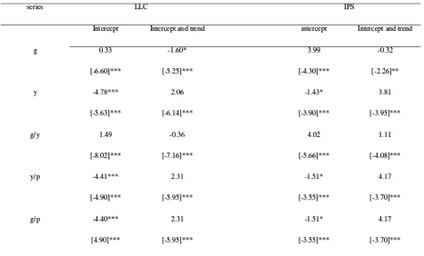
estimate 5 versions of Wagner’s law. Also prior to estimation of our panel regressions, we
perform conventional panel unit root tests of Levin et al. (2002) and Im et al. (2002) and the
reported results in Table 1 indicate that none of the series is integrated of an order higher than
I(1), which is a property of the time series which allows compatible of the variables with our
[image:10.595.66.532.324.606.2]designated methodology.
Table 1: Unit root test results
series LLC IPS
Intercept Intercept and trend intercept Intercept and trend
g 0.33
[-6.60]***
-1.60*
[-5.25]***
3.99
[-4.30]***
-0.32
[-2.26]**
y -4.78***
[-5.63]***
2.06
[-6.14]***
-1.43*
[-3.90]***
3.81
[-3.95]***
g/y 1.49
[-8.02]***
-0.36
[-7.16]***
4.02
[-5.66]***
1.11
[-4.08]***
y/p -4.41***
[-4.90]***
2.31
[-5.95]***
-1.51*
[-3.55]***
4.17
[-3.70]***
g/p -4.40***
[4.90]***
2.31
[-5.95]***
-1.51*
[-3.55]***
4.17
[-3.70]***
Notes: significance codes “***”, “**”, “*” are 1%, 5% and 10% critical levels, respectively. Test statistics for first difference reported in [].
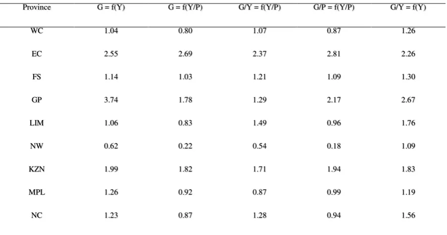
Our empirical analysis is summarized in the following three steps. In the first step, we
compute the F-statistics bounds tests for all individual provinces for all 5 estimated versions
exceed their respectively 10 percent upper critical levels hence implying that we cannot rely
ARDL framework for empirical purposes. Encouragingly enough, this also implies that out
[image:11.595.67.519.185.422.2]suggested SPSM framework for panel cointegration can be utilized as an alternative.
Table 2: “Bounds” test for cointegration for individual provinces
Province G = f(Y) G = f(Y/P) G/Y = f(Y/P) G/P = f(Y/P) G/Y = f(Y)
WC 1.04 0.80 1.07 0.87 1.26
EC 2.55 2.69 2.37 2.81 2.26
FS 1.14 1.03 1.21 1.09 1.30
GP 3.74 1.78 1.29 2.17 2.67
LIM 1.06 0.83 1.49 0.96 1.76
NW 0.62 0.22 0.54 0.18 1.09
KZN 1.99 1.82 1.71 1.94 1.83
MPL 1.26 0.92 0.87 0.99 1.19
NC 1.23 0.87 1.28 0.94 1.56
The 10% critical values for bounds test are as follows: I(0) – 3.02, I(1) – 3.51.
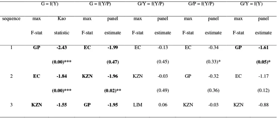
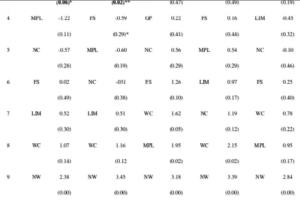
In the second step of our empirical process, we proceed to implement the SPSM to
cointegration discussed in the previous section of the paper. To achieve this we firstly arrange
the individual F-statistics obtained in Table 2, from the statistics with the highest rejection
(largest F-statistic) to that of the lowest statistic (smallest F-statistic). Note that this has been
done for all provinces and for all 5 estimated versions of Wagner’s law which are reported in Table 3. Also note that the optimal lags for each of the regressions has been selected based on
the minimization of Schwarz information criterion. Then afterwards, we compute the
associated Kao (1999) panel statistics for all 5 versions of Wagner’s law, firstly for the entire
panel (as indicate by sequence 1), and then on a reducing balance, where we firstly remove
the province which produces the highest individual F-statistic, which in our case is Gauteng
We then re-calculate the Kao (1999) test statistic for the reduced panel and then
remove the provinces with the second largest F-statistic, which is now Eastern Cape for
Peacock-Wiseman (1961) and Mann (1968) versions, Gauteng for the Gupta version (1967)
version and KZN for the Goffman (1968) and Musgrave (1969) versions. Even though by
description we are only supposed to carry out the process until the panel Kao cointegration
test static fails to detect any cointegration effects, we decide to carry out this procedure
throughout all diminishing panel sets for completeness and confirmation sake.
After completing the entire procedure, as reported in Table 3, we observe that panels
inclusive of GP, EC and KZN produces significant cointegration effects whereas when these
provinces are removed from the panel, the remaining panel regressions indicate no significant
cointegration effects. However, we are quick to note that the results obtained for the
Musgrave (1969) and Gupta (1967) versions are not as optimistic as none of the computed
Kao (1999) statistics can reject the null hypothesis of no panel cointegration whereas that for
the Mann (1968) version is only significant with Gauteng included in the panel sample and
insignificant once this province is removed from the panel. It is therefore only for the
Peacock-Wiseman (1961) version and (2) Pryor (1969) versions that all three provinces (GP,
EC and KZN) are found to contribute to the finding of significant Wagner effects in the
[image:12.595.70.518.558.751.2]panel.
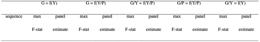
Table 3: Kao’s (1999) panel cointegration tests on sequential panels
G = f(Y) G = f(Y/P) G/Y = f(Y/P) G/P = f(Y/P) G/Y = f(Y)
sequence max
F-stat
Kao
statistic
max
F-stat
panel
estimate
max
F-stat
panel
estimate
max
F-stat
panel
estimate
max
F-stat
panel
estimate
1 GP -2.43
(0.00)***
EC -1.99
(0.47)
EC -0.13
(0.45)
EC -0.34
(0.33)*
GP -1.61
(0.05)*
2 EC -1.84
(0.00)***
KZN -1.96
(0.02)**
KZN -0.03
(0.49)
GP -0.32
(0.36)
EC -1.17
(0.12)
(0.06)* (0.02)** (0.47) (0.49) (0.19)
4 MPL -1.22
(0.11)
FS -0.59
(0.29)*
GP 0.22
(0.41)
FS 0.16
(0.44)
LIM -0.45
(0.32)
5 NC -0.57
(0.28)
MPL -0.60
(0.19)
NC 0.56
(0.29)
MPL 0.54
(0.29)
NC -0.10
(0.46)
6 FS 0.02
(0.49)
NC -031
(0.38)
FS 1.26
(0.10)
LIM 0.97
(0.17)
FS 0.25
(0.40)
7 LIM 0.52
(0.30)
LIM 0.51
(0.30)
WC 1.62
(0.05)
NC 1.19
(0.12)
WC 0.78
(0.22)
8 WC 1.07
(0.14)
WC 1.16
(0.12
MPL 1.95
(0.02)
WC 2.15
(0.02)
MPL 0.95
(0.17)
9 NW 2.38
(0.00)
NW 3.45
(0.00)
NW 3.18
(0.00)
NW 3.39
(0.00)
NW 2.84
(0.00)
Notes: significance codes “***”, “**”, “*” are 1%, 5% and 10% critical levels, respectively.
p-values reported in ().
In the final step of our empirical procedure, we then estimate the long-run
coefficients, the short-run coefficients and the error correction terms for our PMG regressions
performed for all versions of Wagner’s law. These estimates are respectively reported in Tables 4, 5 and 6 and as previously mentioned the optimal lag selection as determined by the
Schwarz information criterion is (1,0) for all models. To also ensure robustness of our
estimated regressions we use the Newly-West heteroscedasticity and autocorrelation
consistent (HAC) estimators. Recall, that according to our rule of thumb, regression estimates
are supposed to be produced only for ‘panels’ which passed the cointegation tests reported in Table 3, and yet, for completeness sake we report all regression estimates on the entire
samples of reducing panels. However, to ensure the ease of interpretation, we report the
estimates of panels which passed the cointegration tests in bold. A can be observed from
Table 4, all long-run regressions for the panels of GP, EC and KZN from the
Peacock-Wiseman (1961) and Pryor (1969) version as well as those inclusive of the GP for the Mann
positive long-run estimates are comparable to those previously obtained in the studies of
Ogbonna (2009), Menyah and Wolde-Rufael (2012), Odhiambo (2015) and Phiri (2017).
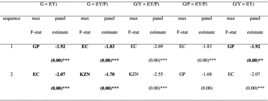
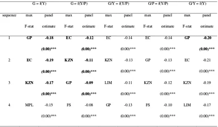
In turning to the associated short-run coefficients and error correction terms for these
significant panels as reported in Tables 4 and 5, respectively, we firstly highlight that all
panels obtain negative and highly statistically significant estimates for the short-run
coefficients. Similar findings of a negative coefficient estimate are found in the study of
Chipaumire et al. (2014). Moreover, all ‘significant’ panel regressions produce error correction terms which have the correct negative and statistically significant estimates hence
implying reversion back to steady-state equilibrium in the face of an exogenous shock to the
system. What can be collectively drawn from our empirical exercise is that while Wagner’s law only holds for South African provinces over the long-run, such effects o not exist over
the short-run where government size is negatively correlated with economic growth or it’s
variant measures. However, our analysis also shows that Wagner’s law only holds if the GP,
EC and KZN provinces are included in the panels, hence implicating that these provinces are
responsible for any observed Wagner’s law at aggregated levels.
What is further important to realize from our empirical exercise, is that if we had
relied strictly on individual ARDL regressions, we would have come to the conclusion of no
evidence of Wagner’s effect at provincial level, seeing that none of the obtained F-statistics
testing cointegration managed to reject the “no cointegration” null hypothesis. On the other
hand, if we strictly relied on panel regression estimates for the entire provinces we would
have concluded that fiscal budgets are mutual sustainable across the provinces. We therefore
[image:14.595.64.520.675.750.2]consider our empirical exercise as some-what of a success.
Table 4: Long-run estimates
G = f(Y) G = f(Y/P) G/Y = f(Y/P) G/P = f(Y/P) G/Y = f(Y)
sequence max
F-stat
panel
estimate
max
F-stat
panel
estimate
max
F-stat
panel
estimate
max
F-stat
panel
estimate
max
F-stat
panel
1 GP 2.64
(0.00)***
EC 3.38
(0.00)***
EC 2.11
(0.00)***
EC 3.11
(0.00)***
GP 2.19
(0.00)***
2 EC 2.60
(0.00)***
KZN 3.90
(0.00)***
KZN 2.48
(0.00)***
GP 3.48
(0.00)***
EC 2.16
(0.00)***
3 KZN 2.65
(0.00)***
GP 4.79
(0.00)***
LIM 3.06
(0.00)***
KZN 3.22
(0.00)***
KZN 2.12
(0.00)***
4 MPL 2.62
(0.00)***
FS 4.67
(0.00)***
GP 3.05
(0.00)***
FS 3.73
(0.00)***
LIM 2.03
(0.00)***
5 NC 2.54
(0.00)***
MPL 4.56
(0.00)***
NC 2.73
(0.01)**
MPL 3.66
(0.00)***
NC 2.01
(0.00)***
6 FS 2.44
(0.00)***
NC 4.61
(0.01)**
FS 2.60
(0.02)**
LIM 3.74
(0.01)**
FS 1.99
(0.00)***
7 LIM 2.39
(0.00)***
LIM 4.31
(0.02)**
[image:15.595.69.518.582.751.2]WC 2.52
(0.03)*
NC 3.74
(0.01)**
WC 2.07
(0.00)***
8 WC 2.37
(0.00)***
WC 4.30
(0.02)**
MPL 2.50
(0.09)*
WC 3.51
(0.02)**
MPL 2.77
(0.01)**
9 NW 2.93
(0.00)***
NW 3.82
(0.24)
NW 2.39
(0.38)
NW 3.39
(0.22)
NW 3.62
(0.24)
Notes: significance codes “***”, “**”, “*” are 1%, 5% and 10% critical levels, respectively.
p-values reported in ().
Table 5: Short-run estimates
G = f(Y) G = f(Y/P) G/Y = f(Y/P) G/P = f(Y/P) G/Y = f(Y)
sequence max
F-stat panel estimate max F-stat panel estimate max F-stat panel estimate max F-stat panel estimate max F-stat panel estimate
1 GP -1.92
(0.00)***
EC -1.83
(0.00)***
EC -2.69
(0.00)***
EC -1.83
(0.00)***
GP -1.92
(0.00)**
2 EC -2.07
(0.00)***
KZN -1.70
(0.00)***
KZN -2.55
(0.00)***
GP -1.68
(0.00)
EC -2.07
3 KZN -1.84
(0.00)***
GP -1.63
(0.00)***
LIM -2.50
(0.00)***
KZN -1.79
(0.00)***
KZN -1.79
(0.00)***
4 MPL -1.78
(0.00)***
FS -1.74
(0.00)***
GP -2.57
(0.00)***
FS -1.73
(0.00)***
LIM -1.74
(0.00)***
5 NC -1.56
(0.00)***
MPL -1.83
(0.00)***
NC -2.73
(0.00)
MPL -1.82
(0.00)***
NC -1.60
(0.00)***
6 FS -1.34
(0.00)***
NC -1.63
(0.00)***
FS -2.59
(0.00)***
LIM -1.63
(0.00)***
FS -1.69
(0.00)***
7 LIM -1.36
(0.00)***
LIM -1.38
(0.00)***
WC -2.72
(0.00)***
NC -1.82
(0.00)***
WC -1.77
(0.00)***
8 WC -1.50
(0.00)***
WC -1.54
(0.00)***
MPL -2.82
(0.00)***
WC -1.56
(0.00)***
MPL -1.09
(0.00)***
9 NW -1.18
(0.00)***
NW -1.53
(0.00)***
NW -2.36
(0.00)***
NW -1.51
(0.00)***
NW -1.13
(0.00)***
Notes: significance codes “***”, “**”, “*” are 1%, 5% and 10% critical levels, respectively.
[image:16.595.69.519.488.751.2]p-values reported in ().
Table 6: Error correction estimates
G = f(Y) G = f(Y/P) G/Y = f(Y/P) G/P = f(Y/P) G/Y = f(Y)
sequence max
F-stat panel estimate max F-stat panel estimate max F-stat panel estimate max F-stat panel estimate max F-stat panel estimate
1 GP -0.18
(0.00)***
EC -0.12
(0.00)***
EC -0.14
(0.00)***
EC -0.14
(0.00)***
GP -0.20
(0.00)***
2 EC -0.19
(0.00)***
KZN -0.11
(0.00)***
KZN -0.13
(0.00)***
GP -0.13
(0.00)***
EC -0.21
(0.00)***
3 KZN -0.17
(0.00)***
GP -0.09
(0.00)***
LIM -0.11
(0.00)***
KZN -0.12
(0.00)***
KZN -0.19
(0.00)***
4 MPL -0.15
(0.00)***
FS -0.08
(0.00)***
GP -0.13
(0.00)***
FS -0.10
(0.00)***
LIM -0.17
5 NC -0.10
(0.00)***
MPL -0.09
(0.01)***
NC -0.12
(0.00)***
MPL -0.12
(0.00)***
NC -0.18
(0.00)***
6 FS -0.10
(0.00)***
NC -0.07
(0.00)***
FS -0.13
(0.00)***
LIM -0.09
(0.00)***
FS -0.21
(0.00)***
7 LIM -0.11
(0.01)**
LIM -0.07
(0.05)*
WC -0.15
(0.00)***
NC -0.11
(0.00)***
WC -0.23
(0.05)*
8 WC -0.15
(0.00)***
WC -0.11
(0.02)**
MPL -0.18
(0.00)***
WC -0.13
(0.00)***
MPL -0.14
(0.03)*
9 NW -0.18
(0.00)***
NW -0.13
(0.02)**
NW -0.15
(0.00)***
NW -0.15
(0.00)***
NW -0.08
(0.00)***
Notes: significance codes “***”, “**”, “*” are 1%, 5% and 10% critical levels, respectively.
p-values reported in ().
5. CONCLUSION
In our study we extend the SPSM method and implement it within the setting of a
cointegration framework. We consider this an important contribution to literature more
particularly for researchers investigating economic relationships which require the use of
time series estimation techniques and yet have short associated time series data to work with.
In such instances, panel time series data consisting of multiple countries or regions can be
used and through the use of the SPSM technique demonstrated in this paper, one can retain
the power of panel regression estimates yet retain the heterogeneity advantages presented by
individual country/region estimates. Through an application of the SPSM method of
cointegration to Wagner’s law for South African provinces, we find that panels consisting of
Gauteng, Eastern Cape and Kwazulu-Natal find significant Wagner effects whereas, when
these provinces are removed from the panels, cointegration effects are absent.
REFERENCES
and national income for three African countries”, Applied Economics, 29, 543-550.
Anyikwa I., Haaman N. and Phiri A. (2018), “Persistence in suicides of G20 countries: SPSM approach to three generations of unit root tests”, MPRA Working Paper No. 87790, July.
Calitz E., Du Plessis S. and Siebrits F. (2014), “Fiscal sustainability in South Africa: Will history repeat itself?”, Journal of Studies in Economics and Econometrics, 38(3), 55-78.
Chang T., Wu T. and Gupta R. (2015), “Are hosue prices in South Africa really
nonstationary? Evidence form SPSM-based panel KSS test with Fourier function”, Applied Economics, 47(1), 32-53.
Chipaumire G., Ngirande H., Method M. and Ruswa Y. (2014), “The impact of government spending on economic growth: Case South Africa”, Mediterranean Journal of Social
Sciences, 5(1), 109-118.
Chortareas G. and Kapetanois G. (2009), “Getting PPP right: Identifying mean-reverting real
exchange rates in panels”, Journal of Banking and Finance, 30(2), 390-404.
Goffman I. (1968), “On the empirical testing of Wagner’s law: A technical note”, Public
Finance, 23(3), 359-364.
Gupta S. (1967), “Public expenditure and economic growth: A time series analysis”, Public
Finance, 22, 423-461.
Im K., Pesaran M. and Shin Y. (2003), “Testing for unit roots in heterogeneous panels”,
Journal of Econometrics, 115(1), 53-74.
Kao C. (1999), “Spurious regression and residual-based tests for cointegration in panel data”,
Lee K. (2014), “Is per capita GDP stationary in China? Sequential panel selection method”,
Economic Modelling, 37, 507-517.
Levin A., Lin C. and Chu J. (2002), “Unit root tests in panel data: asymptotic and finite sample properties”, Journal of Econometrics, 108(1), 1-24.
Li X., Tang (2014), “CO2 emissions converge in the 50 U.S. states – Sequential panel
selection method”, Economic Modelling, 40, 320-333.
Maddala G. (1987), “Limited dependent variable models using panel data”, Journal of Human Resources, 22(3), 307-338.
Mann A. (1980), “Wagner’s law: An econometric test for Mexico 1926-1976”, National Tax
Journal, 33, 189-201.
Menyah K. and Wolde-Rufael Y. (2012), “Wagner’s law revisited: A note from South
Africa”, South African Journal of Economics, 80(2), 200-208.a
Musgrave R. (1969), “Fiscal systems”, New Haven: Yale University Press.
Narayan P., Nielsen I. and Smyth R. (2008), “Panel data, cointegration, causality and Wagner’s law: Empirical evidence form Chinese provinces”, China Economic Review, 19(2),
297-307.
Odhiambo N. (2015), “Government spending and economic growth in South Africa”, Atlantic Economic Journal, 43(3), 393-406.
Ogbonna B. (2009), “Testing Wagner’s law of government size for South Africa”, Journal of
Peacock A. and Wiseman J. (1961), “The growth of public expenditure in the United Kingdom”, Princeton: Princeton University Press.
Pesaran H., Shion Y and Smith R. (1999), “Pooled mean group estimation of dynamic heterogenous panels”, Journal of the American Statistical Association, 94(446), 621-634.
Pesaran M., Shin Y. and Smith R. (2001), “Bounds testing approaches to the analysis of level relationships”, Journal of Econometrics, 16(3), 289-326.
Phiri A. (2017), “Nonlinearities in Wagner’s law: Further evidence from South Africa”, International Journal of Sustainable Economy, 9(3), 231-249.
Pryor F. (1969), “Public expenditures in communist and capitalist nations”, London: George
Allen and Unwin.
Ziramba E. (2008), “Wagner’s law: An econometric test for South Africa, 1960-2006”, South