Munich Personal RePEc Archive
Heterogeneous effects of the
implementation of macroprudential
policies on bank risk
Ely, Regis Augusto and Tabak, Benjamin Miranda and
Teixeira, Anderson Mutter
Federal University of Pelotas, Getulio Vargas Foundation, Federal
University of Goias
17 June 2019
Online at
https://mpra.ub.uni-muenchen.de/94546/
Heterogeneous e
ff
ects of the implementation of macroprudential policies on
bank risk
Regis A. Elya,∗
, Benjamin M. Tabakb, Anderson M. Teixeirac
aDepartment of Economics at Federal University of Pelotas, Pelotas-RS, Brazil
bSchool of Public Policy and Government at Getulio Vargas Foundation, Bras´ılia-DF, Brazil cDepartment of Economics at Federal University of Goi´as, Goiˆania-GO, Brazil
This version: June 17, 2019
Abstract
In this article, we analyze the effect of a set of 12 macroprudential policies on the risk-taking of banks using a large number of countries and banks. Our empirical results show that, although on
average these policies reduce risk-taking, the effects are quite heterogeneous and vary considerably depending on the instrument implemented, market concentration, size of banks, liquidity, leverage
and different levels of risk. Structural policies, such as limits on asset concentration and interbank exposures, are the most effective in terms of financial stability. Borrower based policies, such as loan-to-value and debt-to-income ratios, also have a positive effect on stability. Concentration limits tend to be more effective for larger and more leveraged banks, while loan-to-value and debt-to-income ratios are more effective in concentrated markets. We also show that there seems to be a greater effect through the leverage channel for policies that are most effective in reducing risk-taking.
Keywords:financial stability, macroprudential policies, bank regulation
JEL classification: G21, G28, L10
✩Regis A. Ely gratefully acknowledges financial support from the CNPq foundation (Grant no. 153270/2018-7).
∗
Corresponding author: Regis A. Ely.
1. Introduction
The financial crisis of 2008/2009 demonstrated that the microprudential approach was insuf-ficient to regulate financial systems since it did not take systemic risk into account. Over the last
few years, a series of macroprudential policies focus on limiting risk-taking, especially for the
larger and more interconnected banks that could generate systemic risk. However, there is a gap
in the literature because we know very little about the effects of these macroprudential policies on risk-taking and the behavior of banks in general.
In this article we contribute to the literature by analyzing the effect of macroprudential policies on bank risk-taking, using a large number of countries and banks. Our results show that the effects are quite heterogeneous and vary considerably depending on the instruments implemented, bank
characteristics and market structures. However, the empirical results suggest that specific
macro-prudential measures are effective in reducing risk-taking of the more significant and more essential banks in each country’s banking system.
Another contribution was to analyze a large number of macroprudential policies and to
com-pare the effects of the adoption of each of them on bank risk-taking. Our empirical results show that although on average, the effects reduce the risk-taking, the impact of the measures varies substantially. Structural policies, such as limits on asset concentration and interbank exposures,
are the most effective in terms of stability. Borrower based policies, such as loan-to-value and debt-to-income ratios, also have a positive effect on stability. Concentration limits tend to be more effective for bigger and more leveraged banks, while loan-to-value and debt-to-income ratios are more effective in concentrated markets. All structural and borrower-based policies appear to be less effective for more stable banks, while capital based policies, such as countercyclical capital requirements, capital surcharges on systematically essential banks, dynamic loan-loss provisions,
and leverage ratios, have mixed effects.
Asset-based policies, such as limits on domestic and foreign currency loans and reserve
re-quirements, are the least effective, especially for riskier banks. While reserve requirements produce positive effects on stability when interacted with size, liquidity, and leverage, limits on domestic and foreign currency loans have adverse effects on stability, especially for riskier banks.
leverage channel in most cases where macroprudential policies were effective in reducing systemic risk or risk-taking. Thus, macroprudential policies limit bank leverage, reducing their exposure to
risk.
Our final contribution concerns the approach used to identify the causal relationship between
the adoption of macroprudential policies and the effects on risk-taking. Our approach relies on nearest neighbor matching using propensity scores before estimating a system-GMM method to
account for the selection bias on the implementation of each policy and the presence of temporal
persistence in the Z-score measure. For each country that implemented the policy (treated), we
used propensity score matching to include a non-treated country using variables related to bank
characteristics and macroeconomic and institutional factors.
In assessing the effects of these macroprudential policies on bank risk-taking, this article re-lates to recent literature, such asBruno et al.(2017),Cerutti et al.(2017a),Akinci and
Olmstead-Rumsey(2018) andAltunbas et al.(2018). Our results corroborate the results for countries with
diverse institutional sets and financial markets, highlighting the main measures taken to mitigate
risk for most vulnerable banks.
We particularly study the effects of the implementation of a set of 12 MPs on the risk-taking of banks of several countries and measure the heterogeneity of the effects under different prisms: con-centration, size of banks, liquidity, leverage and different levels of risk. In addition to this primary objective, we also seek to measure how the effect of the implementation of regulatory instruments changes for different market structures and characteristics of the banking system especially about variables such as concentration, size of banks, liquidity, and leverage. We evaluate which
regu-latory instruments are most effective for banks with excessive risk-taking. We also break down the impact of MPs on risk-taking, in order to determine whether the effects of such policies are due to an increase in bank returns or to a decrease in the volatility of these returns. We propose a
proper identification approach in order to measure the effects of the implementation of MPs from cross-country data.
To carry out this study, we used a comprehensive accounting database of more than 15,000
banks in 45 different emerging and developed countries, with data ranging between 1995 and 2014. These data, obtained from the BankScope database (BVD-IBCA), contain all the
accounting characteristics of the banks. The macroprudential policy database, developed byCerutti
et al. (2017a) and built from the Global Macroprudential Policy Instruments (GMPI) survey
con-ducted during 2013/2014 and 2016/2017, was also used, as well as cross-country macroeconomic and institutional data, obtained from the World Bank and the Heritage Foundation.
To measure the effects of MPs on the financial stability of banks we used a risk measure called Z-score, which is a proxy for financial stability and is inversely proportional to the probability of
bank failure. The measures of liquidity, leverage, and size of the banks, as well as the
Herfindahl-Hirschman concentration index, were obtained through the accounting data. The use of these risk
and concentration measures are common in the literature (Demirg¨uc¸-Kunt and Huizinga, 2010;
Fazio et al.,2015;Tabak et al.,2012).
In order to estimate and identify the effects of the implementation of the MPs, we first perform a propensity score matching with the countries in our sample to account for possible selection bias
of the implementation of each policy. Then we estimate a system-GMM model, as formulated in
Arellano and Bover(1995) andBlundell and Bond(1998), since the bank risk variable (Z-score) is
a measure that presents temporal persistence and whose lagged values are usually correlated with
the fixed effect in panels with short T and long N (Arellano and Bond,1991). Lastly, we perform the decomposition of the Z-score measure and add interactions to understand the mechanisms
through which the MPs affect the risk-taking of banks.
We organize the remainder of the paper as follows. In Section 2we present a brief literature
review and discuss our contribution. Section3discusses macroprudential policies and their
defini-tions. Section5presents an overview of the data used to perform our empirical exercise. Section4
presents the methods and identification strategy. Section6presents and discusses empirical results
and Section7concludes the paper.
2. Literature review
The global financial crisis of 2007-2008 rekindled the debate on how to regulate and supervise
banks and other financial institutions to ensure financial stability. Macroprudential policies (MPs)
regarding credit limits, capital reserves, and bank balance-sheet restrictions were part of the
bank-ing regulations discussed at Basel III (BIS, 2011). Both emerging and developed countries have
associated with adverse shocks to the real side of the economy (Borio,2010;Claessens,2015).
Before the global financial crisis (GFC), financial regulation of banks and other financial
inter-mediaries was strongly focused on instruments aimed at reducing the risk of individual bankruptcy,
not of the financial system as a whole. However, the bankruptcy of a large financial institution may
jeopardize the solvency of the entire system (systemic risk). Tabak et al. (2016) found evidence
that banking supervision is positively correlated with bank stability, thus contributing to mitigate
systemic risk.
According to Freixas et al.(2015), microprudential regulation that focused solely on the
sol-vency of financial institutions largely ignored the externalities of the financial sector and the real
sector for the entire macroeconomic cycle and, therefore, was not able to respond to the aggregate
dynamics of the interconnections of the banking system as a whole.
According to Brunnermeier et al. (2009), De Nicolo et al. (2012) and Cerutti et al. (2017a),
the main sources of banking risk that justify the implementation of MPs are externalities that
exist in the financial sector and market failures. These externalities can be associated with three
essential factors: i) vulnerabilities that may arise due to strategic interaction of banks during a
cycle of financial expansion; ii) deterioration of the accounting and collateral balance sheets due
to a general fall in asset prices in periods of financial contraction cycles; and iii) the propagation
of systemic shocks into the financial market due to its interconnectivity.
Therefore, a set of macroprudential policies was proposed to identify and minimize the risks
to systemic stability. The need to infer the effectiveness of such policies is thus one of the critical challenges for policymakers and scholars.1.
The works of Moreno(2011), Galati and Moessner(2013),Lim et al. (2011), Claessens et al.
(2013), Claessens(2015) and Freixas et al.(2015) summarize the main policies implemented by
both developing and developed countries, as well as their meanings and objectives towards
miti-gating systemic risk, arising from the procyclicality and interconnectivity between financial
insti-tutions.
In addition to this literature, whose objective was to present and describe the central
macropru-1In addition to the challenge of assessing the effectiveness of MPs,Altunbas et al.(2018) lists the challenge of
dential policies, there is increasing literature regarding the impact of macroprudential regulation
on the behavior of bank loans and financial stability. Here, one can separate this literature into
three broad groups. The first group includes studies called cross-countries. In one of these studies,
Lim et al.(2011) examined the links between macro-prudential policies and the development of
the credit market, as well as bank leverage. They found evidence suggesting that policies limiting
loan-to-value (LTV) and debt-to-income ratios (DTI), in addition to policies establishing capital
reserve requirements and dynamic provisioning rules, are associated with reductions in credit and
leverage procyclicality. Tabak et al. (2017) found positive effects of more significant capital re-serves of banks on profitability, although these effects proved to be negative in cases where banks have excessive capital reserves.
Other cross-country studies include Claessens et al. (2013), who showed that the maximum
limits of LTV, DTI and maximum limits for loans in foreign currency were effective in reducing the growth of bank leverage and asset prices;Zhang and Zoli(2016) who confirmed a high effect of the LTV measure in containing growth in property prices, credit, and bank leverage;Aiyar et al.(2014)
and Gropp et al. (2018) who showed that in response to stricter capital requirements, regulated
banks reduced borrowing, while unregulated banks even increased their amount borrowed; and
lastly, Auer and Ongena (2016), who found that an additional capital requirement on real estate
loans led to growth in the commercial lending channel.
In addition to this empirical evidence,Cerutti et al.(2017a), using an IMF survey of 12 MPs in
119 countries between 2000 and 2013, found that it was generally the emerging countries that most
adopted such policies. Besides, policies such as DTI and LTV are associated with the decline in
credit growth, especially real estate lending. The authors also confirmed that MPs help in managing
the business cycle, but work less efficiently in recessive periods. Also noteworthy is the work of Jim´enez et al.(2017), who investigated the impact of pro-cyclical banking regulation on lending to
companies2.
The second group of studies focuses on investigating the effect of one or a few MPs, but for specific countries. Among these studies we can highlightIgan and Kang(2011), who investigated
the effectiveness of only the LTV and DTI instruments in South Korea. Wong et al. (2011) also
2
Other cross-country studies investigating the effectiveness of a set of MPs areAkinci and Olmstead-Rumsey
used only LTV and DTI instruments, but investigated their effects on real estate credit and real estate prices in Hong Kong. Camors et al.(2014) investigated the effect of capital withdrawal in Uruguay in 2008, while Aiyar et al. (2014) confirmed a strong effect of capital requirement on loans for UK banks.
In line with our objective,Altunbas et al.(2018) investigated the effectiveness of MPs in miti-gating the risk behavior of banks. Their evidence suggested that MPs have a significant impact on
bank risk. Also, the authors also suggest that responses to changes in MPs differ between banks and are highly dependent on their specific characteristics. We contribute to this article by
mea-suring the effectiveness of such policies on banks that are excessively risky, as well as develop an identification approach to deal with selection bias.
Among the main theoretical studies, we highlight Begenau (2016), who developed a general
equilibrium model to analyze the effect of MPs on bank loans. Kashyap et al. (2014) presented a general equilibrium model and showed the effects of the capital requirement measure on bank risk. In this paper, the authors modify the Diamond and Dybvig(1983) bank run model. Lastly,
Elenev et al.(2018) elaborated a macroeconomic model to estimate and evaluate how MPs impose
restrictions on firms and bank leverage.
3. Macroprudential indicators
The database used to identify the adoption of macroprudential policies in different countries came from a survey of the International Monetary Fund (IMF) called the Global Macroprudential
Policy Instruments (GMPI) conducted in 2013/2014 and 2016/2017. These data comprise a series of more than 100 detailed questions on the adoption of 17 different MPs that were answered by the central banks and monetary authorities of 140 IMF member countries. Cerutti et al. (2017a)
used this survey and verified the consistency of the responses with an earlier version for 2011,
in order to construct a database with binary indicators (dummy variables) on the use of 12 MPs
between 2000 and 2013 for 120 different countries. Later, the authors updated the database to include observations from 2014 to 2017 and increased the list of countries to 160.
We combine the MPs database with banking and macroeconomic data for 1995 to 20003for 45
countries selected based on data availability4.
The 12 MPs were classified as: (i) Countercyclical capital requirements (CTC); (ii) capital
surcharges on systematically important banks (SIFI); (iii) Dynamic loan-loss provisions (DP); (iv)
Leverage ratio (LEV); (v) Limits on domestic currency loans or credit growth limits (CG); (vi)
Foreign and/or countercyclical reserve requirements (RR REV); (vii) Limits on foreign currency loans (FC); (viii) Caps on loan-to-value ratio (LTV CAP); (ix) Caps on debt-to-income ratio (DTI);
(x) Concentration limits (CONC); (ix) Limits on interbank exposure (INTER); and (xii) Tax on
financial institutions (TAX).
The instruments CTC, SIFI, DP, and LEV, rely on capital requirements, provisioning, and
surcharges. The first case refers to countercyclical capital requirements, which aim to ensure that
the capital requirements of the banking sector take into account the macroeconomic and financial
environment in which banks operate. Thus, this instrument aims to protect the banking sector
during periods of excess aggregate credit growth, which are usually associated with increased
systemic risk. On the other hand, in periods of credit restriction, capital requirements may be
lower, so as not to affect the performance of the real sector of the economy.
The second measure, SIFI, imposes a surcharge on the capital requirements for financial
institu-tions that are considered systematically important. Therefore, the requirements are more significant
for those banks that have greater importance in terms of systemic risk. This higher requirement
makes it possible to minimize the probability of bankruptcy or liquidity problems associated with
these banks5.
The third measure, DP, is similar to CTC in terms of the dynamics of the operation of the
instrument. However, it requires specific provisioning for defaults on loan agreements, allowing
the creation of a financial reserve in periods of economic growth which can be used to cover
defaults that occur in periods of recession6. The last capital-based measure is LEV, which prevents
banks from exceeding a fixed minimum leverage ratio.
will require a set of 5 initial annual observations. We discard these observations for the estimation of the final models, as described in section4.
4We describe the steps to obtain our final sample, as well as the description of bank and macroeconomic data in
section5.
5
Further details on the regulatory standards involving CTC and SIFI measures are available inBIS(2011).
6
The instruments CG, FC, and RR REV, are asset-based and impose restrictions on financial
sector balance sheets, assets, and liabilities. CG calls for limits on domestic currency loans, while
FC limits foreign currency loans, reducing vulnerability to foreign-currency risks. Reserve
re-quirements (RR REV) are traditionally used in emerging countries, especially in Brazil, with the
objective of controlling the multiplication of money through the imposition of compulsory deposits
with the Central Bank of part of the demand deposits of financial institutions7.
The instruments LTV CAP and DTI are borrower-based and impose restrictions on the
bor-rower, instrument or activity. LTV CAP refers to a cap on the percentage of the value of an asset
that can be financed by a bank loan to ensure a minimum collateral value for a loan, usually set at
about 70% or 80%. The DTI ratio is an alternative instrument that imposes minimum levels on the
expected capacity of borrowers to pay their debts, to control excessive borrowing by banks8.
CONC and INTER are structural tools aimed at addressing vulnerabilities from
interconnect-edness and limiting contagion of the financial system. CONC limits the fraction of assets
concen-trated to a limited number of borrowers, while INTER limits the fraction of liabilities held by the
banking sector or by individual banks. The last instrument, TAX, imposes taxes on the revenue of
financial institutions in order to control credit growth, mitigate economic cycles or correct systemic
externalities.
Although other MPs may be in use in some countries other than those discussed in this paper,
an analysis of the effect of these 12 instruments on the risk attitude of banks provides a general understanding of the leading MPs currently in use in both developed and emerging countries9.
4. Methods and identification strategy
In this paper, we evaluate the impact of each of the 12 MPs on bank stability individually.
The decision to implement a macroprudential policy is not a random one and depends on the
banking system characteristics, as well as the macroeconomic and institutional variables of each
country. This decision usually generates a self-selection bias because countries that have banks
with a higher probability of default will usually implement more MPs. In order to reduce this bias,
7A detailed study of the implementation and effects of compulsory reserves in Brazil are available inGlocker and
Towbin(2015).
8
Morgan et al.(2015) study the implementation of these policies in detail for Asian countries.
9
we estimated our models in two stages. First, we performed a propensity score matching through
nearest neighbor, thus obtaining one similar matched country for each treated one. Second, we ran
a dynamic panel data regression with instruments (System-GMM) to estimate the effect of MPs on bank stability taking into account the autoregressive nature of the Z-score, as well as the time and
fixed effects for individual banks.
The propensity score is the probability of a treatment being assigned conditional on observed
baseline characteristics. It allows the design and analysis of an observational (nonrandomized)
study so that it mimics the specific characteristics of a randomized controlled trial. Condition
on the propensity score, the distribution of observed baseline covariates will be similar between
treated and untreated subjects. In general, this method allows two countries to be compared, one in
the control group and the other in the treatment group, with very similar observable characteristics,
with the main factor that differentiates them is the implementation of the specific MP analyzed. This method has the potential to reduce or eliminate possible confounding factors and allows the
estimation of the effect of each MP on bank risk-taking and stability.
We first estimate the probability of treatment (propensity scores) through a logit regression
for each MP. To perform these first stage regressions we used one observation for each country.
We take the mean of the accounting, macroeconomic and institutional variables across banks and
years10. The dependent variable of these regressions was a dummy that identifies countries where
the policy is under use in any year of the sample. After performing these regressions, we matched
each treated country with an untreated one with a similar propensity score using a nearest
neigh-bor algorithm. After these procedures done for each of the 12 MPs, we run the System-GMM
regressions with bank-level data for only treated and matched countries.
We used three different strategies for the matching according to the macroprudential policy: i) CTC and SIFI were implemented only in 2013, so we were able to match countries based on
pretreatment variables (from 2000 to 2012), and then we perform a 1:1 matching without
replace-ment; ii) DP, DTI, LEV, CG, INTER, RR REV, FC, and TAX is implemented throughout the entire
period of analysis, so we used all years while performing the first stage regressions, and then
per-formed a 1:1 matching without replacement; iii) LTV CAP and CONC were the most implemented
10
policies, and since we had a limited number of untreated countries we used all years in the first
stage regressions and performed a 1:1 matching with replacement.
After the matching, we estimated dynamic panel regressions with instrumental variables
(System-GMM) to obtain the effects of the 12 MPs on bank stability and, through interactions, we also evaluated how these effects change for variables such as the size of banks, liquidity, leverage, and concentration. We also used dummies to identify banks with excessive risk (first quintile of the
Z-score) and higher stability (last quintile of the Z-Z-score) interacting them with the treatment variable
in order to assess the heterogeneity of the effect of the MPs across different risk-taking quintiles. Through this estimation, it was possible to identify which instruments had the most impact on
the excessively risky banks, which had a higher probability of bankruptcy and which affected the systemic risk the most. Lastly, we also performed auxiliary estimates and robustness tests, which
included the decomposition of the risk measure known as Z-score, as well as specification tests for
the System-GMM model.
A fixed effect panel data model can have a significant correlation with the lagged dependent variable, so we use a System-GMM model instead, as proposed by Arellano and Bover (1995).
With the inclusion of the instruments proposed byBlundell and Bond(1998), we reduce the
endo-geneity bias due to the presence of the lagged dependent variable in our regressions. This model
also allows the use of lagged variables as instruments for the bank characteristics that are
consid-ered endogenous or predetermined. In order to ensure a proper specification of the models and
reduce the problem of too many instruments (Roodman, 2009), we apply a principal component
analysis (PCA) on the instrument matrix. We use the PCA scores as instruments for the
System-GMM estimation, followingBontempi and Mammi(2012).
The risk-taking measure that we use as the dependent variable is the logarithm of the Z-score.
We calculate the Z-score using the following formula:
Z-scoreikt =
ROAikt+Equity Ratioikt
σikt(ROA)
, (1)
where ROAikt and Equity Ratioikt are the return on asset and equity over assets in period t for
Since we have annual data, the standard deviation of the return on asset is calculated through a
rolling window using the five prior observations, which is why the data for the period from 1995
to 1999 (used to calculate the standard deviation ofROA in 2000) is not present in the estimation
of the econometric models. This strategy for constructing the Z-score is similar to that adopted
byDelis et al.(2012) and recommended for annual data inLi and Malone (2016). The Z-score is
inversely proportional to a bank’s probability of bankruptcy and has the interpretation of a measure
of financial stability, or as the distance, a bank is from insolvency. Many studies in the literature
have used the Z-score as a risk measure (Mercieca et al.,2007;Laeven and Levine,2009;Houston
et al.,2010;Demirg¨uc¸-Kunt and Huizinga,2010;Fazio et al.,2015).
Since we used rolling windows to calculate the Z-score, we expected it to present a highly
correlated structure. In order to remove this correlation, we included two lags of the dependent
variable in all models. For each MP we estimate eight different System-GMM models: i) one baseline regression to evaluate the overall impact of the MP on bank stability; ii) four regressions
where we interacted the dummy of the MP with either the size of banks, the liquidity ratio, the
leverage ratio and the HHI loans concentration index, in order to assess how the effectiveness of the MPs changes according to these variables; iii) one regression where we interacted dummies
that identified the excessively risky and higher stable banks with the MP, in order to assess the
heterogeneity of the effect across different risk-taking quintiles; iv) two regressions where we used the baseline model but with the components of the Z-score as dependent variables, in order to
understand how the policies affected the Z-score of the banks. Our baseline regression has the following specification:
ln(Z-score)ikt = αi+β1ln(Z-score)ik,t−1+β2ln(Z-score)ik,t−2+β3MPkt
+ Bank Controls′
iktβ5+Macro Controls
′
ktβ6+εikt (2)
where the subscriptsi,kandtrefer to bank, country and year, respectively; ln(Z-score)iktis aN×1
vector of the logarithm of the bank Z-score, considering we have a total of N observations in our
sample;MPktis aN×1 vector with the dummy of the macroprudential policy; Bank Controls
′
iktis
a N× pmatrix with pcontrol variables for the bank characteristics; Macro Controls′
matrix with qmacroeconomic and institutional control variables for the countries in the sample;
αi andβj are the coefficients to be estimated; andεikt is the error term. Our four regressions with
interactions have the following base specification:
ln(Z-score)ikt = αi+β1ln(Z-score)ik,t−1+β2ln(Z-score)ik,t−2+β3MPkt
+ β4(MPkt·Xikt)+Bank Controls
′
iktβ5+Macro Controls
′
ktβ6+εikt (3)
whereXiktis aN×1 vector with the variable to be interacted with MPkt, either size, liquidity,
lever-age or concentration. The other variables are the same as in equation2. Our quintile regressions
have the following specification:
ln(Z-score)ikt = αi+β1ln(Z-score)ik,t−1+β2ln(Z-score)ik,t−2+β3MPkt
+ β4(MPkt·Higher riskikt)+β5(MPkt·Higher stabilityikt)+β6Higher riskikt
+ β7Higher stabilityikt+Bank Controls
′
iktβ8+Macro Controls
′
ktβ9+εikt (4)
where Higher riskikt and Higher stabilityikt are dummies that identifies whether the bank has a
Z-score in the first or last quintile, respectively. We interacted these dummies with the dummy of the
macroprudential policy in order to investigate heterogeneity between different levels of risk-taking. Finally, we also ran regressions with the same specification of equation 2 but with the
com-ponents of the Z-score as a dependent variable: the logarithm of the risk-adjusted return on assets
(ROA/σ(ROA)) and the logarithm of the risk-adjusted equity ratio (Equity Ratio/σ(ROA)). With
these regressions, we were able to understand how MPs affect the bank Z-scores. We also report the Hansen test and the serial correlation tests of first and second order in each System-GMM
regression to ensure a proper specification of the instruments.
5. Data description
All accounting data used to calculate risk-taking, size, liquidity, leverage, concentration and other
specific characteristics of banks are from BankScope, a financial database distributed by the
BVD-IBCA. The data is converted into US dollars to ensure accounting uniformity across different coun-tries. The information is annual and covers the period between 1995 and 2014. The first five years
are used only for the calculation of the risk measure known as Z-score, and the 2000 to 2014 data
are used to estimate the econometric models.
We added country-level data to the bank accounting data to reflect both the implementation of
macroprudential regulation policies discussed in the previous section and the macroeconomic and
institutional information. The macro-prudential policy database was obtained from Cerutti et al.
(2017a) through the Global Macroprudential Policy Instruments (GMPI) survey, from the
Interna-tional Monetary Fund (IMF) in 2013/2014 and 2016/2017, while macroeconomic and institutional data were obtained from the database of the World Bank and Heritage Foundation, respectively.
Initially, the BankScope database contained more than 20,000 commercial banks, cooperative
and savings banks from 201 different countries, while theCerutti et al. (2017a) macroprudential policy database included 160 countries. After merging the two databases and removing countries
without information on MPs, some filters and cutouts were used to eliminate outliers and countries
with few banks, guaranteeing a representative sample of the banks in the countries analyzed.
First, we removed the consolidated balance sheets of the banks with unconsolidated balance
sheets, in order to avoid duplication of observations in the data11. Banks with less than five balance
sheets were then removed, as well as countries with less than ten different banks. The first choice is vital in order to ensure a sufficient number of observations to calculate the risk measure, Z-score. We choose countries with at least ten banks to avoid that specific characteristic of a bank
could influence the results obtained for a particular country. Moreover, at the same time to select an
appropriate group of emerging and developed countries. Finally, we remove missing values, and all
of the accounting variables relevant to the study were winsorized at 1%, limiting the extreme values
represented by the 1% and 99% percentiles, in order to reduce the effects of possible spurious
11
The option to work with the unconsolidated balance sheets avoided the possibility of data duplication (if a Bank A owns a Bank B, the consolidated balance sheet reports the assets of both banks, requiring the identification and removal of the unbound balance sheet of Bank B from the database). In cases where there was no unconsolidated balance sheet, we use the consolidated balance sheets. This strategy follows the line of articles such asMicco et al.
outliers.
With these procedures, an unbalanced panel data sample was obtained, comprised of 16,255
banks in 45 countries. In addition to the dummy variables that describe the implementation of
MPs, which take value one after the implementation in a country in a given year, the econometric
models included different variables to control for specific characteristics of the banks related to management and decision-making that could change over time. These variables include the
log-arithm of total assets (Size), the ratio of liquid assets to total assets (Liquid Ratio), the degree of
leverage, measured by the debt to equity ratio (Leverage), the ratio of bank deposits to total assets
(Deposit Ratio), an efficiency measure given by the ratio of total expenses to net bank loans (Cost Ratio), and the ratio of total loans to total assets (Loan/Assets). The first three variables were also
interacted with the dummies of MPs to verify how their effect changed for banks with different sizes, liquidity, and leverage.
We also use the following macroeconomic and institutional variables, which vary over time and
according to the country: GDP per capita growth; the ratio of total exports and imports to GDP;
the concentration of the loan banking market, measured by the HHI index; the aggregate ratio of
equity to assets; the aggregate ratio between loans and deposits; and the property rights index. The
purpose of using these variables was to control the temporal changes in the specific macroeconomic
and institutional characteristics of the countries in the dynamic panel models. The HHI index was
also interacted with the dummies of MPs to verify how their effect changed according to different market structures.
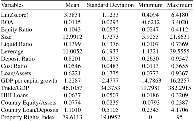
Table1includes the descriptive statistics of the variables that we use in this study, including the
two components of the Z-score: the return on assets (ROA) and the equity ratio. Table2lists the
countries in our sample as well as the number of banks and MPs implemented in each country; the
mean values of the logarithm of the Z-score and its components by country; and the mean values
of the variables that we interact with the macroprudential dummies. Finally, Table 3 reports the
percentage of countries in this sample that implemented each of the MPs described in section 3
between 2000 and 2014.
We can see from Table 1 that the sample includes countries with different institutional levels and stages of development. The property rights index, measured on a scale of 100, ranges from 0
The use of winsorized accounting variables made it possible to reduce extreme values in equity,
liquidity, deposits, costs, and loan ratios. For a fair comparison of the accounting data, the mean
value of certain selected variables for each country can be visualized in Table2.
The three countries with the most significant number of sampled banks were the United States,
Germany, and Russia, with China and Thailand standing out for having the largest banks on average
as measured by the logarithm of total assets. The logarithm of the Z-score is a measure inversely
proportional to the probability of bank failure, so a higher average value represents more bank
sta-bility in the country. Thus, countries such as Switzerland, Germany and the United Arab Emirates
have banks with the lowest probability of bankruptcy, while Latvia, Argentina, and Romania have
less stable banks.
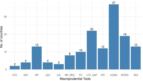
Table 3presents the percentage of implementation for each of the 12 MPs between 2000 and
2014, while Figure1refers to the number of countries that adopted each policy in at least one year
of the sample. The most adopted policies were the borrower concentration limits (CONC) and the
cap on loan-to-value ratio (LTV CAP). CONC was adopted by 45.45% of the sampled countries in
2000, increasing to more than 50% of adoption after 2001, while LTV CAP was adopted by almost
50% of the countries by the year 2014. Of the 45 countries, 37 and 22 countries implemented
CONC and LTV CAP in at least one year of the sample, respectively. Specific instruments, such
as CTC and SIFI, were adopted only in recent years, making it possible to compare and design
more adequate identification strategies, while other instruments were adopted by certain countries
over the entire period of analysis, allowing only a comparison with banks of other countries.
6. Results
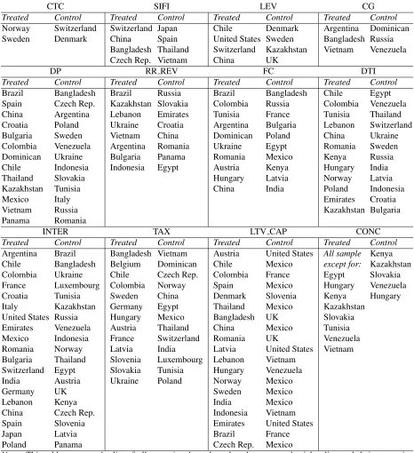
Before estimating the regressions of equations 2, 3 and 4, we first performed the propensity
score matching for each MP in order to obtain a reduced sample of countries. Table 4 presents
the list of countries that implemented each MP and their respective untreated matched country
based on the estimations of the propensity scores and the algorithm of nearest neighbor discussed
in section4.
Several MPs, such as INTER, LTV CAP, and DP, were implemented in many countries, whereas
others, such as CTC and CG, only in a limited number of countries. In all cases, we used the
countries for the same treated country depending on the MP implemented. For example, Spain
may be a better control country for China (SIFI), but since it is considered a treated country in
LTV CAP, the next available best match is Mexico. However, in the case of the LEV policy, Spain
is not used as a control for China. We follow this procedure because the matching also seeks to
predict the dependent variable as best as possible.
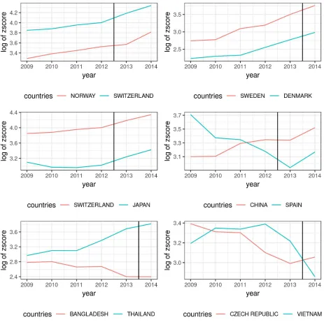
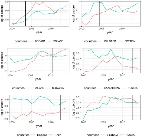
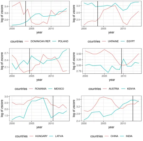
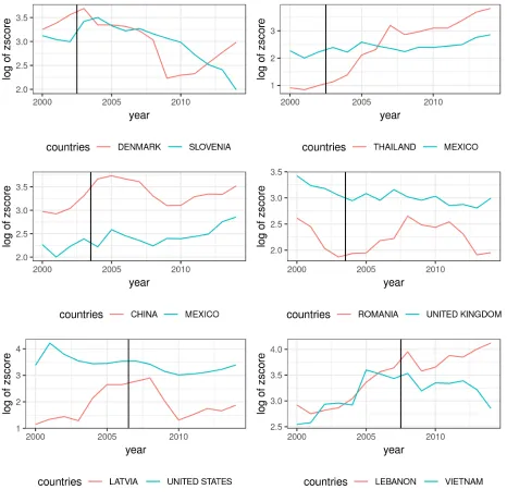
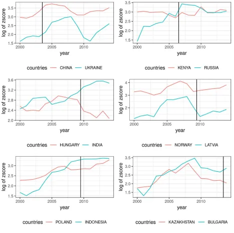
Figures2 to10show the evolution of the logarithm of the Z-score for selected countries that
implemented the MPs in the middle of the sample (in red) and their respective untreated matched
country (in blue). As stated in section4, we matched the countries with their nearest neighbor using
the propensity scores. The vertical line shows the year of implementation. We present the number
of countries that implemented each MP in Figure 1. In all cases, the common trends hypothesis
seems to hold as there is a parallel trend before the implementation of the policy. In our view, these
figures show that the quality of the matching procedure is relatively good.
In many cases, there was a similar trend for the Z-score for treated and matched countries
before the intervention. The changes in the trend after the intervention may give us a clue about
the effect of each MP, although we still need to control for the dynamics of the Z-score, fixed effects of banks, and many possible observed characteristics of banks and countries which may change
over time. We do this in Tables5 to16, where we estimated the System-GMM models after the
matching for each of the 12 MPs.
Tables 5to 16present the eight different specifications of the System-GMM models for each MP. In column one of each table, we show the results of the baseline model estimated through
equation 2. In columns two to five, we show the results of the regressions in equation 3, where
we interacted the MP dummy with the size of banks, the liquidity ratio, the leverage ratio, and
the HHI loans concentration index. In column six we show the results of the regression estimated
through equation4, where we assessed the heterogeneous effects of the policies for different levels of bank risk-taking. Finally, in columns seven and eight we estimated the same regression for
equation2, but using the logarithm of the risk-adjusted return on assets and the logarithm of the
risk-adjusted equity ratio as dependent variables, respectively. The variable Xt in the second line
of the regressions refers to the variables interacted with the MP dummy, such as size, liquidity,
leverage, HHI, and the dummy that identifies banks in the first quintile of the Z-score (Higher
the risk-adjusted Equity Ratio (in column eight).
The number of observations and banks in each table changes according to the number of treated
banks, since we performed propensity score matching before the estimation of the models for
each MP. We also report p-values of the Hansen and serial correlation tests. As we can see, all
regressions have the correct specification at the level of significance of 5% according to those
tests. We included year dummies in all regressions, but the coefficients of the year dummies and the constant are not present in all tables due to space considerations.
The baseline regressions show a positive effect of structural and borrower based policies on bank stability, such as: SIFI, LTV CAP, CONC, INTER (Tables6,12,14,15, respectively). When
we check for the heterogeneous effects of these policies, we observe that SIFI has a higher effect for more liquid banks (column three of Table6), that LTV CAP has a higher effect for banks with more liquidity and leverage (columns three and four of Table 12), and that CONC has a higher
effect for larger and more leveraged banks (columns two and four of Table14). All of these three policies have a lower effect for more stable banks. We also find positive effects of DP for highly leveraged banks (column four of Table7), LEV for concentrated markets (column five of Table
8), and DTI for banks with more size, liquidity and leverage, and for more concentrated markets
(columns two, three, four and five of Table13). DTI also show less effect for more stable banks (column six of Table13).
These results are in line with the evidence that loan-to-value or debt-to-income limits can be
useful in leaning against real estate booms, can help curb housing price growth (Hartmann,2015;
Zhang and Zoli, 2016;Kuttner and Shim,2016) and help reduce excess volatility in the economy
(Gelain et al.,2013).
Some of these policies, especially asset-based, show a significant negative effect on bank sta-bility when considering the baseline regression, such as CG, RR REV and FC (Tables 9, 10, 11,
respectively). CG and FC have a more negative effect for banks with higher risk (column six of Tables9and11). Although CG seems to have a negative effect on stability for all cases, RR REV and FC have a positive effect for larger and more leveraged banks (columns two and four of Tables 10and11). The policy based on revenue taxes only has a negative effect on stability for very con-centrated markets (column five of Table16). Finally, CTC (Table5) seems to have no significant
Our evidence has some similarities with the findings ofAltunbas et al.(2018), since there was
no significant effect of capital based policies on banking stability, such as CTC, DP, and LEV, except SIFI. Popoyan et al. (2017) also found that minimum capital requirements and
counter-cyclical capital buffers are a practical regulatory framework, whileJim´enez et al.(2017) found that dynamic provisioning smooths credit supply cycles and, in hard times, supports firm performance.
According to a survey conducted byGalati and Moessner(2018), many different studies found some evidence of borrower-targeted macroprudential policies having some effects on intermediate targets of these macroprudential policies, such as housing price growth and housing credit growth.
By contrast, empirical evidence on the effects of macroprudential capital flow management tools is less conclusive and more mixed.
Similar toBrandao-Marques et al.(2018), we also ran the same regressions but with the
com-ponents of the Z-score as dependent variables in columns 7 and 8 of Tables 5 to 16. The two
components are the risk-adjusted return on assets and the risk-adjusted equity ratio. We use the
latter as a proxy for leverage. We can see that while SIFI, LTV CAP, RR REV, and FC mainly
af-fected the Z-score through the leverage channel, CG, CONC, and INTER also affected the Z-score through the return on assets.
Our results show that policies that impose limits on domestic and foreign currency loans, such
as CG and FC, may hurt bank stability. Both types of policies hurt the equity ratio, which reflects
the fact that banks reduce their equity when their loan operations diminish. Limits on loans granted
domestically also seem to have a negative on the return relation of banks, decreasing the
risk-adjusted return on assets.
On the other hand, essential tools that aim to address vulnerabilities from interconnectedness
and contagion of the financial system, such as CONC and INTER, have a positive effect on bank stability, increasing the risk-return relation of banks and the risk-adjusted equity ratio. Specific
borrower-based instruments, such as LTV CAP, also have a positive effect on bank stability, pri-marily through the leverage channel.
In tables17to20we grouped the MPs into four significant groups: capital based policies, such
as CTC, SIFI, DP and LEV; asset-based policies, such as CG, RR REV and FC; borrower-based
policies, such as LTV CAP and DTI; and structural policies, such as CONC and INTER. We then
of those policies are under use in the country. The dummy equals one whenever the policy is active.
The results support the findings of the previous regressions, since we found a positive and
sig-nificant effect of structurally based instruments on banking stability, while asset-based instruments have a negative effect. We also found some evidence of a positive relationship between borrower based instruments and bank stability, which, as exposed in table 12, may be due to the positive
effect of LTV CAP. Finally, capital-based policies seem to have mixed effects on risk-taking, since CTC and LEV do not present significant effects, while SIFI and DP increase stability.
7. Conclusions
In this article, we studied the effects of the implementation of a set of 12 macroprudential policies on the risk-taking of banks for several countries using an identification approach that
relied on a nearest neighbor matching with propensity scores and a system-GMM model. We
found that macroprudential policies have considerably heterogeneous effects depending on bank characteristics and market structures. Variables such as concentration, size of banks, liquidity,
leverage and different levels of risk are essential to explain how macroprudential policies may affect the risk-taking behavior of banks.
Our main results suggest that the most effective policies in terms of stability were structural-based, such as limits on the concentration of assets and interbank exposure. Borrower-based
poli-cies, such as loan-to-value and debt-to-income ratios, as well as capital surcharges on
systemati-cally important banks also have a positive effect on stability. The least effective policies seem to be those that impose limits on domestic and foreign currency loans. They hurt stability, especially
for banks with excessive risk-taking.
There seem to be a more substantial effect through the leverage channel in most cases in which macroprudential policies are effective in reducing risk-taking. The risk-return relation of a bank is also essential to explain the negative effect of limits on domestic credit on bank stability.
This article adds to the literature that seeks to evaluate how different macroprudential policies affect the risk-taking incentives of banks. Our results support the application of these policies in countries with the most diverse institutional sets and financial market characteristics and also
highlights the main measures to be taken to mitigate risk to most vulnerable banks.
banking market characteristics of countries into account. Although some of those policies can
sub-stantially reduce the risk-taking of banks, they can also produce some unintended consequences.
Gurrea-Mart´ınez and Remolina(2019) found that higher capital requirements may reduce access
to finance, especially in emerging markets, creating financial exclusion problems. It is essential
to highlight that macroprudential policies that reduce risk-taking may also decrease credit growth
and hamper economic growth. The opportunity cost of such policies may be a relevant topic for
future research.
References
Aiyar, S., Calomiris, C., Wieladek, T., 2014. Does Macro-Prudential Regulation Leak? Evidence
from a UK Policy Experiment. Journal of Money, Credit and Banking 46, 181–204.
Akinci, O., Olmstead-Rumsey, J., 2018. How effective are macroprudential policies? an empirical investigation. Journal of Financial Intermediation 33, 33 – 57.
Altunbas, Y., Binici, M., Gambacorta, L., 2018. Macroprudential policy and bank risk. Journal of
International Money and Finance 81, 203–220.
Arellano, M., Bond, S., 1991. Some Tests of Specification for Panel Data: Monte Carlo Evidence
and an Application to Employment Equations. The Review of Economic Studies 58 (2), 277–
297.
Arellano, M., Bover, O., 1995. Another look at the instrumental variable estimation of
error-components models. Journal of Econometrics 68 (1), 29–51.
Auer, R., Ongena, S., 2016. The Countercyclical Capital Buffer and the Composition of Bank Lending. BIS Working Papers No 593.
Aysan, A. F., Fendo˘glu, S., Kilinc¸, M., 2015. Macroprudential policies as buffer against volatile cross-border capital flows. The Singapore Economic Review 60 (01), 1550001.
Begenau, J., 2016. Capital Requirements, Risk Choice, and Liquidity Provision in a Business Cycle
BIS, Jun. 2011. Basel III: A global regulatory framework for more resilient banks and banking
systems. Tech. rep.
Blundell, R., Bond, S., Nov. 1998. Initial conditions and moment restrictions in dynamic panel
data models. Journal of Econometrics 87 (1), 115–143.
Bontempi, M. E., Mammi, I., 2012. A strategy to reduce the count of moment conditions in panel
data gmm. MPRA Working Paper 40720.
Borio, C., 2010. Implementing a macroprudential framework: Blending boldness and realism. BIS
Working Papers No 22.
Brandao-Marques, L., Correa, R., Sapriza, H., 2018. Government support, regulation, and risk
taking in the banking sector. Journal of Banking & Finance.
Brunnermeier, M. K., Crockett, A., Goodhart, C. A. E., Persaud, A. D., Shin, H.-s. (Eds.), 2009.
The fundamental principles of financial regulation. No. 11 in Geneva reports on the world
econ-omy. ICMB, Internat. Center for Monetary and Banking Studies, Geneva, oCLC: 837319149.
Bruno, V., Shim, I., Shin, H. S., 2017. Comparative assessment of macroprudential policies.
Jour-nal of Financial Stability 28, 183–202.
Camors, C. D., Peydro, J.-L., Tous, F. R., 2014. Macroprudential and Monetary Policy: Loan-Level
Evidence from Reserve Requirements. Mimeo. Universitat Pompeu Fabra.
Cerutti, E., Claessens, S., Laeven, L., 2017a. The use and effectiveness of macroprudential policies: New evidence. Journal of Financial Stability 28, 203–224.
Cerutti, E., Dagher, J., Dell’Ariccia, G., 2017b. Housing finance and real-estate booms: A
cross-country perspective. Journal of Housing Economics 38, 1–13.
Cizel, J., Frost, J., Houben, A., Wierts, P., 2016. Effective macroprudential policy: Cross-sector substitution from price and quantity measures. Tech. Rep. 498, Netherlands Central Bank,
Re-search Department.
Claessens, S., 2015. An Overview of Macroprudential Policy Tools. Annual Review of Financial
Claessens, S., Ghosh, S. R., Mihet, R., 2013. Macro-prudential policies to mitigate financial system
vulnerabilities. Journal of International Money and Finance 39 (C), 153–185.
Crowe, C., Dell’Ariccia, G., Igan, D., Rabanal, P., 2013. How to deal with real estate booms:
Lessons from country experiences. Journal of Financial Stability 9 (3), 300–319.
De Nicolo, G., Favara, G., Ratnovski, L., 2012. Externalities and Macroprudential Policy. IMF
StaffDiscussion Notes 12/05, International Monetary Fund.
Delis, M. D., Tran, K. C., Tsionas, E. G., 2012. Quantifying and explaining parameter
heterogene-ity in the capital regulation-bank risk nexus. Journal of Financial Stabilheterogene-ity 8 (2), 57–68.
Demirg¨uc¸-Kunt, A., Huizinga, H., 2010. Bank activity and funding strategies: the impact on risk
and returns. Journal of Financial Economics 98 (3), 626–650.
Diamond, D. W., Dybvig, P. H., 1983. Bank Runs, Deposit Insurance, and Liquidity. Journal of
Political Economy 91 (3), 401–419.
Elenev, V., Landvoigt, T., Van Nieuwerburgh, S., 2018. A macroeconomic model with financially
constrained producers and intermediaries. Working Paper 24757, National Bureau of Economic
Research.
Fazio, D. M., Tabak, B. M., Cajueiro, D. O., 2015. Inflation targeting: Is IT to blame for banking
system instability? Journal of Banking & Finance 59, 76–97.
Freixas, X., Laeven, L., Peydro, J.-L., 2015. Systemic Risk, Crises, and Macroprudential
Regula-tion. MIT Press Books, The MIT Press.
Galati, G., Moessner, R., 2013. Macroprudential Policy – a Literature Review. Journal of Economic
Surveys 27 (5), 846–878.
Galati, G., Moessner, R., 2018. What Do We Know About the Effects of Macroprudential Policy? Economica 85 (340), 735–770.
Gelain, P., Lansing, K. J., Mendicino, C., 2013. House Prices, Credit Growth, and Excess
Volatil-ity: Implications for Monetary and Macroprudential Policy. International Journal of Central
Glocker, C., Towbin, P., Jun. 2015. Reserve requirements as a macroprudential instrument –
Em-pirical evidence from Brazil. Journal of Macroeconomics 44, 158–176.
Gropp, R., Mosk, T., Ongena, S., Wix, C., 2018. Banks response to higher capital requirements:
Evidence from a quasi-natural experiment. The Review of Financial Studies, Forthcoming.
Gurrea-Mart´ınez, A., Remolina, N., 2019. The Dark Side of Implementing Basel Capital
Require-ments: Theory, Evidence, and Policy. Journal of International Economic Law 22 (1), 125–152.
Hartmann, P., 2015. Real Estate Markets and Macroprudential Policy in Europe. Journal of Money
Credit and Banking 47 (1), 69–80.
Houston, J. F., Lin, C., Lin, P., Ma, Y., 2010. Creditor rights, information sharing, and bank risk
taking. Journal of Financial Economics 96 (3), 485–512.
Igan, D., Kang, H., 2011. Do Loan-to-Value and Debt-to-Income Limits Work? Evidence from
Korea. IMF Working Papers (11/297).
Jim´enez, G., Ongena, S., Peydr´o, J.-L., Saurina, J., 2017. Macroprudential Policy, Countercyclical
Bank Capital Buffers, and Credit Supply: Evidence from the Spanish Dynamic Provisioning Experiments. Journal of Political Economy 125 (6), 2126–2177.
Kashyap, A. K., Tsomocos, D. P., Vardoulakis, A. P., 2014. How does macroprudential regulation
change bank credit supply? Tech. Rep. 20165, National Bureau of Economic Research, Inc.
Kuttner, K. N., Shim, I., 2016. Can non-interest rate policies stabilize housing markets? Evidence
from a panel of 57 economies. Journal of Financial Stability 26, 31–44.
Laeven, L., Levine, R., 2009. Bank governance, regulation and risk taking. Journal of Financial
Economics 93 (2), 259–275.
Li, X., Malone, C. B., 2016. Measuring Bank Risk: An Exploration of Z-Score. SSRN Electronic
Journal.
Lim, C., Columba, F., Costa, A., Kongsamut, P., Otani, A., Saiyid, M., Wezel, T., Wu, X., 2011.
Macroprudential Policy: What Instruments and How to Use Them? Lessons from Country
Mercieca, S., Schaeck, K., Wolfe, S., 2007. Small European banks: Benefits from diversification?
Journal of Banking & Finance 31 (7), 1975–1998.
Micco, A., Panizza, U., Ya˜nez, M., 2007. Bank ownership and performance. Does politics matter?
Journal of Banking & Finance 31 (1), 219–241.
Moreno, R., 2011. Policymaking from a ’Macroprudential’ Perspective in Emerging Market
Economies. BIS Working Papers No 336.
Morgan, P., Regis, P. J., Salike, N., 2015. Loan-to-Value Policy as a Macroprudential Tool: The
Case of Residential Mortgage Loans in Asia. ABDI Working Paper Series (528).
Popoyan, L., Napoletano, M., Roventini, A., 2017. Taming macroeconomic instability: Monetary
and macro-prudential policy interactions in an agent-based model. Journal of Economic
Behav-ior & Organization 134, 117–140.
Roodman, D., 2009. A note on the theme of too many instruments*. Oxford Bulletin of Economics
and Statistics 71 (1), 135–158.
Tabak, B., Fazio, D., Ely, R., Amaral, J., Cajueiro, D., 2017. The effects of capital buffers on profitability: An empirical study. Economics Bulletin 17, 1468–1473.
Tabak, B. M., Fazio, D. M., Cajueiro, D. O., 2012. The relationship between banking market
competition and risk-taking: do size and capitalization matter? Journal of Banking & Finance
36 (12), 3366–3381.
Tabak, B. M., Fazio, D. M., de O. Paiva, K. C., Cajueiro, D. O., 2016. Financial stability and bank
supervision. Finance Research Letters 18, 322–327.
Wezel, T., Lau, C., A, J., Columba, F., 2012. Dynamic Loan Loss Provisioning: Simulations on
Effectiveness and Guide to Implementation. IMF Working Papers (12/110).
Wong, T. C., Fong, T., Li, K.F., Choi, H., 2011. LoantoValue Ratio as a Macroprudential Tool
-Hong Kong’s Experience and Cross-Country Evidence. -Hong Kong Monetary Authority
Zhang, L., Zoli, E., 2016. Leaning against the wind: Macroprudential policy in Asia. Journal of
Table 1: Descriptive statistics of the main accounting and macroeconomic variables
Table 2: Mean values of selected variables by country
Countries No. of Ln(Zscore) ROA Equity Size Liquid Leverage HHI No. of
banks Ratio Ratio Loans MPs
Table 3: Macroprudential policy implementation percentages
Year CTC SIFI DP LEV CG RR REV FC LTV CAP DTI CONC INTER TAX 2000 0 0 4.55 4.55 2.27 11.36 6.82 9.09 6.82 45.45 15.91 9.09 2001 0 0 4.44 4.44 2.22 13.33 6.67 8.89 8.89 53.33 20 8.89 2002 0 0 4.44 4.44 2.22 13.33 6.67 8.89 8.89 55.56 20 8.89 2003 0 0 6.67 4.44 2.22 13.33 8.89 13.33 8.89 57.78 22.22 8.89 2004 0 0 8.89 4.44 4.44 13.33 13.33 20 13.33 57.78 22.22 8.89 2005 0 0 11.11 4.44 4.44 15.56 15.56 20 13.33 60 22.22 8.89 2006 0 0 11.11 4.44 4.44 15.56 15.56 20 13.33 62.22 22.22 8.89 2007 0 0 13.33 4.44 4.44 15.56 13.33 22.22 15.56 66.67 28.89 8.89 2008 0 0 13.33 6.67 4.44 13.33 13.33 22.22 15.56 68.89 28.89 11.11 2009 0 0 13.33 6.67 4.44 13.33 13.33 22.22 15.56 71.11 28.89 11.11 2010 0 0 15.56 6.67 4.44 13.33 15.56 28.89 22.22 73.33 31.11 15.56 2011 0 0 17.78 6.67 4.44 13.33 17.78 33.33 24.44 73.33 31.11 28.89 2012 0 0 17.78 8.89 6.67 13.33 17.78 35.56 24.44 73.33 33.33 28.89 2013 2.22 4.44 24.44 8.89 6.67 13.33 20 40 24.44 73.33 33.33 28.89 2014 4.44 8.89 26.67 6.67 6.67 13.64 20 48.89 24.44 82.22 42.22 26.67 Note: This table presents the percentage of countries that implemented each macroprudential policy from 2000 to 2014. Data were obtained fromCerutti et al.(2017a).
[image:30.612.77.537.369.631.2]Table 4: List of countries that implemented each macroprudential policy and its nearest neighbor
CTC SIFI LEV CG
Treated Control Treated Control Treated Control Treated Control Norway Switzerland Switzerland Japan Chile Denmark Argentina Dominican Sweden Denmark China Spain United States Sweden Bangladesh Russia
Bangladesh Thailand Switzerland Kazakhstan Vietnam Venezuela Czech Rep. Vietnam China UK
DP RR REV FC DTI
Treated Control Treated Control Treated Control Treated Control Brazil Bangladesh Brazil Russia Brazil Bangladesh Chile Egypt Spain Czech Rep. Kazakhstan Slovakia Colombia Russia Colombia Venezuela China Argentina Lebanon Emirates Tunisia France Tunisia Thailand Croatia Poland Ukraine Croatia Argentina Bulgaria Lebanon Switzerland Bulgaria Sweden Vietnam China Dominican Poland China Ukraine Colombia Venezuela Argentina Romania Ukraine Egypt Romania Sweden Dominican Ukraine Bulgaria Panama Romania Mexico Kenya Russia Chile Indonesia Indonesia Egypt Austria Kenya Hungary India Thailand Slovakia Hungary Latvia Norway Latvia Kazakhstan Tunisia China India Poland Indonesia
Mexico Italy Emirates Croatia
Vietnam Russia Kazakhstan Bulgaria
Panama Romania
INTER TAX LTV CAP CONC
Treated Control Treated Control Treated Control Treated Control Argentina Brazil Bangladesh Vietnam Austria United States All sample Kenya Chile Bangladesh Belgium Dominican Chile Mexico except for: Kazakhstan Colombia Ukraine Chile Czech Rep. Colombia France Egypt Slovakia France Luxembourg Colombia Norway Spain Mexico Hungary Venezuela Croatia Tunisia Sweden China Denmark Slovenia Kenya Hungary Italy Kazakhstan Germany Egypt Thailand Mexico Kazakhstan
United States Russia Hungary Mexico Bangladesh UK Slovakia Emirates Venezuela Austria Thailand China Mexico Tunisia Mexico Indonesia France Switzerland Romania UK Venezuela Romania Norway Latvia India Latvia United States Vietnam Bulgaria Thailand Slovenia Luxembourg Lebanon Vietnam
Switzerland Egypt Slovakia Tunisia Hungary Venezuela India Austria Ukraine Poland Norway Mexico
Germany UK Sweden Mexico
Lebanon Kenya India Mexico
China Czech Rep. Indonesia Vietnam Spain Slovenia Emirates United States
Japan Latvia Brazil France
Poland Panama Czech Rep. Mexico
Figure 2: CTC and SIFI Matching
Figure 3: DP Matching
Figure 4: LEV, CG and RR REV Matching
Figure 5: FC Matching
Figure 6: LTV CAP Matching
Figure 7: DTI Matching
Figure 8: CONC Matching
Figure 9: INTER Matching
Figure 10: TAX Matching
Table 5: Impact of CTC on banking stability
Dependent Variable: Ln(Z-score) Z-score decomposition Baseline Size Liquidity Leverage HHI Higher risk ROA Equity ratio
(1) (2) (3) (4) (5) (6) (7) (8) CTC 0.230 1.526 0.354 0.460 1.008* 0.041 -0.007 0.274
(0.239) (1.305) (0.346) (0.415) (0.524) (0.168) (0.087) (0.275) CTC·Xt
— -0.100 -1.445 -0.031 -5.093* 0.037 — — (0.089) (1.853) (0.034) (2.668) (0.138)
CTC·Higher stability
— — — — — -0.247 — —
(0.155) Higher risk
— — — — — -0.882*** — —
(0.262) Higher stability
— — — — — 0.969*** — —
(0.253)
Ln(Yt−1) 0.406 0.337 0.320 0.325 0.298 -0.021 0.349 0.244
(0.413) (0.373) (0.377) (0.376) (0.377) (0.307) (0.241) (0.388) Ln(Yt−2) 0.196 0.149 0.139 0.145 0.160 0.146 0.299 0.219
(0.350) (0.342) (0.352) (0.347) (0.357) (0.252) (0.228) (0.317) Size 0.420* 0.381** 0.400** 0.395** 0.404** 0.331* 0.173* 0.454** (0.236) (0.165) (0.168) (0.167) (0.169) (0.175) (0.101) (0.224) Liquid Ratio 3.829 3.104 4.043 3.549 4.367 1.091 -0.185 4.480
(4.781) (3.834) (4.086) (3.913) (4.203) (3.872) (1.606) (5.918) Leverage -0.060*** -0.058*** -0.058*** -0.058*** -0.059*** -0.030* -0.016 -0.054***
(0.021) (0.016) (0.017) (0.016) (0.017) (0.016) (0.015) (0.020) Deposit Ratio -1.053 -0.071 -0.470 -0.160 -0.599 0.327 1.907 0.124
(2.728) (2.465) (2.590) (2.464) (2.588) (1.891) (1.386) (2.845) Cost Ratio 5.131 2.077 -0.306 0.268 0.039 9.080 17.439 5.201
(12.674) (12.681) (13.475) (13.239) (13.888) (11.395) (12.752) (15.716) Loan/Assets 9.668* 8.474** 9.238** 8.789** 9.576** 5.893 3.932** 9.800
(5.312) (3.545) (3.771) (3.578) (3.821) (4.134) (1.803) (6.137) GDP per capita growth -0.045 -0.037 -0.041 -0.043 -0.032 -0.001 -0.037 -0.059
(0.052) (0.040) (0.040) (0.041) (0.037) (0.036) (0.028) (0.052) Trade/GDP 0.023*** 0.021*** 0.021*** 0.021*** 0.022*** 0.017*** 0.018*** 0.022***
(0.006) (0.005) (0.005) (0.005) (0.005) (0.004) (0.004) (0.006) HHI Loans 12.067 8.579 9.747 9.197 9.982 0.246 4.468 12.315 (9.187) (6.452) (6.759) (6.532) (6.835) (7.541) (4.314) (9.564) Country Equity/Assets 33.014 27.701 30.344 29.931 28.801 2.388 23.086* 37.653 (25.128) (18.333) (18.730) (18.765) (18.280) (19.851) (11.813) (25.384) Country Loan/Deposits -1.341 -1.197** -1.248** -1.246** -1.218** -0.673 -1.060** -1.494*
(0.819) (0.605) (0.617) (0.614) (0.604) (0.584) (0.442) (0.765) Property Rights Index -0.073*** -0.068*** -0.070*** -0.068*** -0.072*** -0.035** -0.055*** -0.065***
Table 6: Impact of SIFI on banking stability
Dependent Variable: Ln(Z-score) Z-score decomposition Baseline Size Liquidity Leverage HHI Higher risk ROA Equity ratio
(1) (2) (3) (4) (5) (6) (7) (8) SIFI 0.218** 0.097 -0.208 -0.108 0.380* 0.252** -0.053 0.205**
(0.104) (0.684) (0.235) (0.145) (0.224) (0.123) (0.166) (0.081) SIFI·Xt
— 0.008 2.253** 0.014* -1.039 0.026 — — (0.044) (1.013) (0.008) (1.343) (0.138)
SIFI·Higher stability
— — — — — -0.279*** — —
(0.082) Higher risk
— — — — — -0.658*** — —
(0.200) Higher stability
— — — — — 0.896*** — —
(0.149)
Ln(Yt−1) 0.665*** 0.676*** 0.695*** 0.678*** 0.689*** 0.372** 0.875 0.850***
(0.193) (0.191) (0.220) (0.202) (0.196) (0.188) (0.637) (0.222) Ln(Yt−2) 0.160 0.141 -0.052 0.117 0.159 0.149 -0.479 -0.020
(0.206) (0.212) (0.253) (0.230) (0.211) (0.263) (0.495) (0.207) Size 0.030 0.026 0.073 0.027 0.035 0.021 -0.061 0.005
(0.084) (0.083) (0.078) (0.080) (0.085) (0.069) (0.164) (0.082) Liquid Ratio -2.963 -2.943 -2.679 -4.119 -2.666 -0.850 -10.046 -1.891 (2.808) (2.805) (2.646) (2.608) (2.813) (3.436) (7.947) (2.372) Leverage -0.064*** -0.063*** -0.068*** -0.057*** -0.063*** -0.034** 0.019 -0.050***
(0.012) (0.012) (0.011) (0.010) (0.012) (0.016) (0.019) (0.012) Deposit Ratio 2.577 2.529 4.240** 1.343 2.967 1.784 -2.188 1.716
(2.554) (2.534) (2.070) (2.337) (2.658) (2.779) (4.191) (2.435) Cost Ratio 12.745 11.961 7.397 6.891 15.015 11.064 -32.339 6.976
(12.831) (12.935) (12.171) (13.131) (13.258) (15.212) (21.922) (9.301) Loan/Assets 2.591 2.637 2.857 2.099 2.800 1.885 -4.077 1.997
(2.023) (2.005) (1.942) (1.918) (2.022) (1.763) (4.056) (1.670) GDP per capita growth -0.008 -0.008 0.013 -0.009 -0.009 -0.004 -0.013 -0.021* (0.013) (0.014) (0.016) (0.014) (0.014) (0.016) (0.032) (0.011) Trade/GDP 0.000 0.001 0.007 0.001 -0.000 -0.001 0.012 0.001
(0.004) (0.004) (0.004) (0.004) (0.004) (0.004) (0.008) (0.003) HHI Loans 0.603 0.540 -0.847 0.614 0.687 2.250 2.636 0.538
(1.287) (1.271) (1.976) (1.383) (1.601) (1.587) (2.561) (1.182) Country Equity/Assets -4.982 -5.033 -12.885*** -5.157 -4.546 -2.959 -14.313 -5.180 (4.582) (4.570) (4.727) (4.595) (4.758) (3.552) (9.296) (4.068) Country Loan/Deposits -1.379*** -1.366*** -0.711 -1.353*** -1.436*** -0.521 0.753 -1.006***
(0.469) (0.471) (0.552) (0.478) (0.476) (0.457) (0.721) (0.387) Property Rights Index 0.009 0.009 0.010* 0.005 0.010 0.010 -0.009 0.005