Macroprudential and Monetary Policies: Implications for Financial
Stability and Welfare
Margarita Rubioy
University of Nottingham
José A. Carrasco-Gallegoz
University of Nottingham and Universidad Rey Juan Carlos
January 2014
Abstract
In this paper, we analyze the implications of macroprudential and monetary policies for business
cycles, welfare, and …nancial stability. We consider a dynamic stochastic general equilibrium (DSGE)
model with housing and collateral constraints. A macroprudential rule on the loan-to-value ratio
(LTV), which responds to credit growth, interacts with a traditional Taylor rule for monetary policy.
We compute the optimal parameters of these rules both when monetary and macroprudential policies
act in a coordinated and in a non-coordinated way. We …nd that both policies acting together
unambiguously improves the stability of the system. In both cases, this interaction is welfare improving
for the society, especially in the case of the non-coordinated game. There is though a trade-o¤ between
borrowers and savers. However, borrowers can compensate the saver’s welfare lossà la Kaldor-Hicks
to achieve a Pareto-superior outcome.
Keywords: Macroprudential, monetary policy, welfare, …nancial stability , loan-to-value,
Kaldor-Hicks e¢ ciency
JEL Classi…cation: E32, E44, E58
We would like to thank the discussants and participants of the IREBS Conference 2012, Dynare Conference, ReCapNet Conference, CEUS Workshop 2013, and the IFABS Conference 2013 and the AREUEA session at the ASSA Meetings 2014, as well as the seminar participants at the Bank of England, the Federal Reserve Board, the Federal Reserve Bank of St. Louis, the Central Bank of Luxembourg, the BBVA and the University of Nottingham. Special thanks to Matteo Iacoviello, John Duca, William Dupor, Pau Rabanal, Carlos Thomas, Antonio Mele, Don Schlagenhauf, Daniel Fetter, Christopher Otrok, Rafael Repullo and Jagjit S. Chadha.
mar-"Normally, however, the policy rate is not the only available tool, and much better instruments are
available for achieving and maintaining …nancial stability. Monetary policy should be the last line of
defence of …nancial stability, not the …rst line." Svensson (2012)
1
Introduction
The housing sector is key to understand how the recent …nancial crisis developed and, therefore, crucial for designing recovery and prevention policies. The …nancial crisis was born in the housing sector, grew in the …nancial sector and had its …nal consequences in the real sector. Financial innovations made the …nancial system increasingly complex and interconnected, driving to an expansion of systemic risk, especially through the mortgage market. In this context, when house prices collapsed, micro-prudential policies, those dedicated to prevent the risk from each company, had not managed to avoid the contagion to the real sector and the crisis spread across the …nancial system to the real economy. Then, a great recession a¤ected the whole economy, causing a high level of unemployment. Thus, from a policy perspective, traditional measures have not seemed to be su¢ cient to, …rst, avoid the crisis and, second, have a fast and e¤ective recovery.
As a result, several institutions have implemented macroprudential tools in order to explicitly pro-mote the stability of the …nancial system in a global sense, not just focusing on individual companies. The goal of this kind of regulation is to avoid the transmission of …nancial shocks to the broader economy. Some examples of macroprudential tools are asset-side tools (loan-to-value (LTV) and debt-to-income ratio caps), liquidity-based tools (countercyclical liquidity requirements), or capital-based tools (coun-tercyclical capital bu¤ers, sectorial capital requirements or dynamic provisions).
The LTV requirement is a limit on the value of a loan relative to the underlying collateral (e.g. residential property). Several studies have pointed out that higher LTV ratios combined with higher risk mortgages contributed to the mortgage crisis.1 The LTV is nowadays described as one of the main macroprudential instruments to “mitigate and prevent excessive credit growth and leverage” by the European Systemic Risk Board.2 Within the EU, LTV limits are available in the national prudential framework of 16 Member States.3
The aim of this paper is to evaluate the implications of a macroprudential LTV tool for business
1See, for instance, Abraham et al. (2008) and Duca et al. (2011). 2
See Recommendation of the European Systemic Risk Board (2013).
cycles, …nancial stability, and welfare, as well as its interaction with monetary policy. In order to do that, we use a dynamic stochastic general equilibrium (DSGE) model which features a housing market. The modelling framework consists of an economy composed by borrowers and savers. In particular, our model imposes a limit on borrowing, that is, loans need to be collateralized by a proportion of the value of the assets that the borrower owns. This proportion can be interpreted as an LTV. The macroprudential tool we propose is a rule that automatically reduces loan-to-values when there is a credit boom, therefore limiting the expansion of credit. We assume that there exists a macroprudential Taylor-type rule for the LTV ratio, so that it responds to credit growth, in the spirit of the Basel III regulation which aims at avoiding episodes of excessive credit growth. The monetary policy literature has extensively shown that simple rules result in a good performance; therefore, it seems sensible to apply this kind of rules to macroprudential supervision. This microfounded general equilibrium model allows us to explore all the interrelations that appear between the real economy and the credit market. Furthermore, such a model can deal with welfare-related questions.
In the context of this model, we address several research questions. First, we study the welfare gain for each agent and for the aggregate both for di¤erent levels of a static LTV and for di¤erent values of the reaction parameters of the macroprudential rule. In this way, we discuss the welfare trade-o¤s that may appear between borrowers and savers. Second, we analyze the combination of monetary and macroprudential policy parameters that maximize welfare when the macroprudential regulator and the central bank are coordinated and when they are not. Third, we discuss a Pareto-superior outcome to overcome this trade-o¤ by a system of transfers à la Kaldor-Hicks. Then, we study the dynamics of the model under the optimal parameters. Finally, we graphically convey our results to highlight the e¤ects on macroeconomic and …nancial stability of introducing a new macroprudential policy based on the LTV ratio.
1.1 Related Literature
Our paper …ts into the literature that introduces a macroprudential rule and studies its e¤ects using a DSGE model. Other examples are, for instance, Antipa et al. (2010), who uses a DSGE model to show that macroprudential policies would have been e¤ective in smoothing the past credit cycle and in reducing the intensity of the recession. Another example is Borio and Shim (2007), which emphasizes the complementary role of macroprudential policy to monetary policy and its supportive role as a built-in stabilizer. As well, N.Diaye (2009) shows that monetary policy can be supported by countercyclical prudential regulation. Angelini et al. (2012) uses a DSGE model with a banking sector and shows interactions between capital requirements ratios as a macroprudential tool and monetary policy; they …nd that macroprudential policies are most helpful to counter …nancial shocks that lead the credit and asset price booms. We …nd in our paper that macroprudential policies moderate credit booms. Furthermore, for housing demand shocks, the combination of the macroprudential and the monetary policies manages to control credit without moderating the real e¤ects of the boom.
Since there is an extensive consensus that the origin of the last crisis is related to real estate booms and busts, we have focused on the e¤ects of a macroprudential tool based on the housing sector. However, while most papers in the …eld tend to analyze macroprudential policy through the lens of a counter-cyclical bank leverage rule (e.g. Angelini et al., 2012, Meh and Moran, 2011), in our paper, we study how a key element of the real estate sector, namely the LTV, can serve as a macroprudential tool to improve …nancial stability.4 With a macroprudential orientation, Kannan, Rabanal and Scott (2012) also examines a monetary policy rule that reacts to prices, output and changes in collateral values with a macroprudential instrument based on the LTV; they remark the importance of identifying the source of the shock of the housing or price boom when assessing policy optimality. Funke and Paetz (2012) consider a non-linear version of a macroprudential rule for the LTV. Following this literature, we propose a macroprudential policy based on a Taylor-type automatic rule.5 By analogy with monetary policy, rule-based macroprudential tools – for example, automatic stabilizers – appear appealing (Goodhart, 2004).
One question that arises on the topic is what the objective of the macroprudential authority should be. In recent years, research on macroprudential issues has been wide and intense6 and there an increasing
4Borio et al. (2001) also evaluated limits on the LTV. 5
See Borio and Shim (2007) for a distinction is between rules and discretion in calibrating the tools of macroprudential policy.
6
consensus among academics and policy makers that “the ultimate objective of macro-prudential policy is to contribute to the safeguard of the stability of the …nancial system as a whole”(Recommendation of the European Systemic Risk Board, 2013). In this way, Almeida, Campello and Liu (2006) has studied the e¤ect on the amplitude of the credit cycle results from the mitigating impact of more stringent LTV ratios on the ‘…nancial accelerator’mechanism. They …nd that when a positive income shock leads to an increase in housing prices, the increase in borrowing is expected to be lower in countries with lower LTV ratios. Gelain et al. (2013) evaluate di¤erent policy action that might be used to dampen the resulting excess volatility, including a direct response to house-price growth or credit growth in the central bank’s interest rate rule, the imposition of a more restrictive loan-to-value ratio, and the use of a modi…ed collateral constraint that takes into account the borrower’s wage income. We contribute to this line of research …nding that when we use the macroprudential policy based on the LTV, both the macroeconomy and the …nancial system become more stable. To illustrate that, we construct policy frontiers (Taylor curves) including not only the traditional objectives of monetary policy but also the objective of the macroprudential regulator; …nancial stability. As a measure of …nancial stability we propose the variability of borrowing. This three-dimensional policy frontier shows graphically that the macroprudential policy unambiguously helps to achieve a more stable …nancial and macroeconomic situation.
some light to this issue. As argued by Svensson (2012), we …nd that the non-coordination game delivers higher social welfare and therefore is preferable. When each authority focuses on its own objective, they are more e¤ective in minimizing both macroeconomic and …nancial variability.
Finally, measuring the potential welfare improvement of macroprudential policies has deserved special attention of the academics. Some papers have found that the macroprudential reaction to exogenous shocks can make some people better o¤ (typically borrowers), but not every type of households, or not in all cases. For instance, Lambertini et al. (2013) extends the Iacoviello and Neri (2010) model to incorporate news shocks and a macroprudential rule on the LTV. They …nd that an optimized LTV-ratio rule that responds to credit growth is a Pareto-improving policy compared to the use of a constant LTV ratio. Campbell and Hercowitz (2009), performed a welfare analysis in a DSGE model with borrowers and savers and determined that although high LTV ratios have a direct positive e¤ect on welfare through constraint relaxation, other indirect e¤ects may dominate. Angelini et al. (2012) also discusses the issue and conclude that there is no regime that makes all agents better-o¤. They claim that the optimal (from a welfare perspective) monetary and macroprudential policies may depend on which agent’s welfare is used as objective in the computation of the policies, and also on the type of shock considered. In our paper, we actively contribute to this discussion. We focus on highlighting the welfare trade-o¤s between agents in order to carefully characterize the conditions under which there is room for Pareto improvements. By analyzing welfare for a static LTV, we …nd an LTV threshold below which there is room for Pareto-improving solutions. However, for higher values the trade-o¤ between borrowers and savers appears. Since, a plausible value for the LTV tends to be higher than this value, when calculating the optimal macroprudential rule, we also observe this trade-o¤. Thus, we propose a system of transfers
à la Kaldor-Hicks in which borrowers would compensate savers so that they are indi¤erent between having or not the macroprudential policy. In this way, we obtain a Pareto-superior outcome.7
2
Model Setup
The modeling framework is a DSGE model with a housing market, following Iacoviello (2005). The model is solved by log-linearizing the equilibrium equations around a well-de…ned steady state. The use of DSGE models for the study of macroprudential policies has some limitations and deserves some discussion. When using DSGE models for monetary policy evaluation, the dynamics of the model are matched
7This is the …rst time that this criterion is applied in the macroprudential context albeit it is widely used in regulatory
with the monetary policy transmission mechanism found in the data. However, for macroprudential policies, empirical applications are rare. Furthermore, the macroprudential analysis often refers to the vulnerability of the …nancial system to exceptional events related to non-equilibrium, which cannot be captured by a DSGE model. At the same time, a drawback of DSGE models is that they are in…nite horizons models and therefore are not well suited to incorporate state contingency in a meaningful way. As a result, DSGE models have problems of modelling …nancial intermediation and frictions (Bean, 2009). However, regardless these limitations, DSGE models are often used for macroprudential analysis since they count with other advantages; …rst, they can be compared with a benchmark in which there is only monetary policy. Second, they include many sources of shocks that can be used to check for di¤erent economic trajectories. Moreover, they rely on general equilibrium analysis and are suitable for simulations to study the impact of new policy instruments. Also, calibrated parameters can be altered to test for alternative policy scenarios. And …nally, since DSGE models are microfounded, they are suitable to study welfare issues.8
In our model, the economy features patient and impatient households, a …nal goods …rm, and a central bank which conducts monetary policy. Households work and consume both consumption goods and housing. Patient and impatient households are savers and borrowers, respectively. Borrowers are credit constrained and need collateral to obtain loans. The representative …rm converts household labor into the …nal good. The central bank follows a Taylor rule for the setting of interest rates. The macroprudential authority sets the LTV following a Taylor-type rule.
2.1 Savers
Savers maximize their utility function by choosing consumption, housing and labor hours:
max
Cs;t;Hs;t;Ns;tE0
1
X
t=0
t
s logCs;t+jtlogHs;t
(Ns;t)
;
where s 2 (0;1) is the patient discount factor, E0 is the expectation operator and Cs;t, Hs;t and
Ns;t represent consumption at time t, the housing stock and working hours, respectively. 1=( 1) is
the labor supply elasticity, >0: jtrepresents the weight of housing in the utility function. We assume
thatlog (jt) = log(j) +uJ t, whereuJ tfollows an autoregressive process. A shock tojtrepresents a shock
to the marginal utility of housing.
8
Subject to the budget constraint:
Cs;t+bt+qt(Hs;t Hs;t 1) =
Rt 1bt 1
t
+ws;tNs;t+Ft; (1)
where bt denotes bank deposits, Rt is the gross return from deposits, qt is the price of housing in
units of consumption, and ws;t is the real wage rate. Ft are lump-sum pro…ts received from the …rms.
The …rst order conditions for this optimization problem are as follows:
1
Cs;t
= sEt
Rt
t+1Cs;t+1
; (2)
wts= (Ns;t) 1Cs;t; (3)
jt
Hs;t
= 1
Cs;t
qt sEt
1
Cs;t+1
qt+1: (4)
Equation (2) is the Euler equation, the intertemporal condition for consumption. Equation (4)
represents the intertemporal condition for housing, in which, at the margin, bene…ts for consuming housing equate costs in terms of consumption. Equation (3)is the labor-supply condition.
2.2 Borrowers
Borrowers solve:
max
Cb;t;Hb;t;Nb;t
E0 1
X
t=0
t
b logCb;t+jtlogHb;t
(Nb;t)
;
where b 2 (0;1) is impatient discount factor, subject to the budget constraint and the collateral
constraint:
Cb;t+
Rt 1bt 1
t
+qt(Hb;t Hb;t 1) =bt+Wb;tNb;t; (5)
Et
Rt
t+1
bt=ktEtqt+1Hb;t; (6)
loan-to-value ratio. The borrowing constraint limits borrowing to the present discounted loan-to-value of their housing holdings. The …rst order conditions are as follows:
1
Cb;t
= bEt
Rt
t+1Cb;t+1
+ tRt; (7)
wb;t= (Nb;t) 1Cb;t; (8)
jt
Hb;t
= 1
Cb;t
qt bEt
1
Cb;t+1
qt+1 tktEt(qt+1 t+1): (9)
where t denotes the multiplier on the borrowing constraint.9 These …rst order conditions can be
interpreted analogously to the ones of savers.
2.3 Firms
2.3.1 Final Goods Producers
There is a continuum of identical …nal goods producers that operate under perfect competition and ‡exible prices. They aggregate intermediate goods according to the production function
Yt=
Z 1
0
Yt(z)
" 1
" dz
"
" 1
; (10)
where " > 1 is the elasticity of substitution between intermediate goods. The …nal good …rm chooses Yt(z)to minimize its costs, resulting in demand of intermediate good z:
Yt(z) =
Pt(z)
Pt "
Yt: (11)
The price index is then given by:
Pt=
Z 1
0
Pt(z)1 "dz
1
" 1
: (12)
9
2.3.2 Intermediate Goods Producers
The intermediate goods market is monopolistically competitive. Following Iacoviello (2005), intermediate goods are produced according to the production function:
Yt(z) =AtNs;t(z) Nb;t(z)(1 ); (13)
where 2 [0;1] measures the relative size of each group in terms of labor.10 This Cobb-Douglas production function implies that labor e¤orts of constrained and unconstrained consumers are not perfect substitutes. This speci…cation is analytically tractable and allows for closed form solutions for the steady state of the model. This assumption can be economically justi…ed by the fact that savers are the managers of the …rms and their wage is higher than the one of the borrowers.11
At represents technology and it follows the following autoregressive process:
log (At) = Alog (At 1) +uAt; (14)
where A is the autoregressive coe¢ cient and uAt is a normally distributed shock to technology. We
normalize the steady-state value of technology to 1. Labor demand is determined by:
ws;t=
1
Xt
Yt
Ns;t
; (15)
wb;t=
1
Xt
(1 ) Yt
Nb;t
; (16)
where Xt is the markup, or the inverse of marginal cost.12
The price-setting problem for the intermediate good producers is a standard Calvo-Yun setting. An intermediate good producer sells its good at price Pt(z);and 1 ;2[0;1];is the probability of being
able to change the sale price in every period. The optimal reset pricePt (z) solves:
1
X
k=0
( )kEt t;k
Pt (z)
Pt+k
"=(" 1)
Xt+k
Yt+k(z) = 0; (17)
1 0
Notice that the absolute size of each group is one.
1 1It could also be interpreted as the savers being older than the borrowers, therefore more experienced. 1 2
where "=(" 1)is the steady-state markup. The aggregate price level is then given by:
Pt=
h
Pt1 1"+ (1 ) (Pt)1 "i1=(1 "): (18)
Using(17) and (18);and log-linearizing, we can obtain a standard forward-looking New Keynesian Phillips curvebt= Etbt+1 xbt+u t, that relates in‡ation positively to future in‡ation and negatively
to the markup ( (1 ) (1 )= ). u t is a normally distributed cost-push shock.13
2.4 Monetary Policy
We consider a Taylor rule which responds to in‡ation and output growth:
Rt= (Rt 1) ( t)(1+ R
) (Yt=Yt 1)
R
y R
1
"Rt; (19)
where0 1 is the parameter associated with interest-rate inertia, R 0 and Ry 0measure the response of interest rates to current in‡ation and output growth, respectively. "Rt is a white noise
shock with zero mean and variance "2.
2.5 A Macroprudential Rule for the LTV
In standard models, the LTV ratio is a …xed parameter which is not a¤ected by economic conditions. However, we can think of regulations of LTV ratios as a way to moderate credit booms. When the LTV ratio is high, the collateral constraint is less tight. And, since the constraint is binding, borrowers will borrow as much as they are allowed to. Lowering the LTV tightens the constraint and therefore restricts the loans that borrowers can obtain. Recent research on macroprudential policies has proposed Taylor-type rules for the LTV ratio so that it reacts inversely to variables such that the growth rates of GDP, credits, the credit-to-GDP ratio or house prices. These rules can be a simple illustration of how a macroprudential policy could work in practice. Here, we assume that there exists a macroprudential Taylor-type rule for the LTV ratio, so that it responds to credit growth, in the spirit of the Basel III
regulation which aims at avoiding episodes of excessive credit growth:14
kt=kSS
Bt
Bt 1
k b
; (20)
where kSS is a steady state value for the loan-to-value ratio, and kb 0 measures the response of the
loan-to-to value to the credit growth. This kind of rule would deliver a lower LTV ratio in booms, when there is excessive credit growth, therefore restricting the credit in the economy and avoiding a credit boom derived from good economic conditions (and symmetrically for recessions).15
2.6 Equilibrium
The market clearing conditions are as follows:
Yt=Cs;t+Cb;t: (21)
The total supply of housing is …xed and it is normalized to unity:
Hs;t+Hb;t= 1: (22)
3
Welfare
3.1 Welfare Measure
To assess the normative implications of the macroprudential and monetary policies, we numerically evaluate the welfare derived in each case. As discussed in Benigno and Woodford (2008), the two approaches that have recently been used for welfare analysis in DSGE models include either characterizing the optimal Ramsey policy, or solving the model using a second-order approximation to the structural equations for given policy and then evaluating welfare using this solution. As in Mendicino and Pescatori (2007), we take this latter approach to be able to evaluate the welfare of the two types of agents
1 4
See Kannan et al (2012) for a similar speci…cation.
1 5The feasibility of a implementing a LTV rule at quarterly frequency may be questionable in practice. However, as the
separately.16 The individual welfare for savers and borrowers, respectively, as follows:
Ws;t Et
1
X
m=0
m
s logCs;t+m+jlogHs;t+m
(Ns;t+m)
; (23)
Wb;t Et
1
X
m=0
m
b logCb;t+m+jlogHb;t+m
(Nb;t+m)
; (24)
Following Mendicino and Pescatori (2007), we de…ne social welfare as a weighted sum of the individual welfare for the di¤erent types of households:
Wt= (1 s)Ws;t+ (1 b)Wb;t: (25)
Each agent´s welfare is weighted by her discount factor; respectively, so that the all the groups receive the same level of utility from a constant consumption stream.
However, in order to make the results more intuitive, we present welfare changes in terms of con-sumption equivalents. The concon-sumption equivalent measure de…nes the constant fraction of concon-sumption that households should give away in order to obtain the bene…ts of the macroprudential policy. A pos-itive value means a welfare gain, that is, how much the consumer would be willing to pay to obtain the welfare improvement. Then, when there is a welfare gain, households would be willing to pay in consumption units for the measure to be implemented because it is welfare improving. We use as a benchmark the welfare evaluated when the macroprudential policy is not active and compare it with the welfare obtained when such policy is implemented. The derivation of the welfare bene…ts in terms of consumption equivalent units is as follows:
CEs= exp (1 s) WsM P Ws 1; (26)
CEb = exp (1 b) WbM P Wb 1; (27)
where the superscripts in the welfare values denote the benchmark case when macroprudential policies
1 6
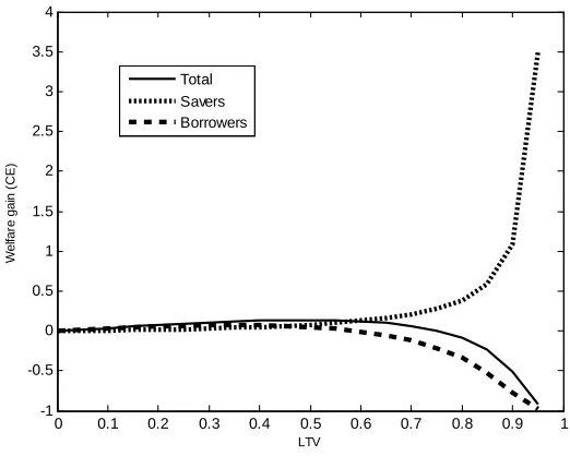
0 0.1 0.2 0.3 0.4 0.5 0.6 0.7 0.8 0.9 1 -1
-0.5 0 0.5 1 1.5 2 2.5 3 3.5 4
LTV
W
el
far
e gai
n (
CE)
[image:14.612.169.430.71.280.2]Total Savers Borrowers
Figure 1: Welfare gains from increasing the LTV ratio, everything else constant. Benchmark case: no macroprudential regulator.
are not introduced and the case in which they are, respectively.17
3.2 Welfare Trade-o¤s
The literature typically …nds that the macroprudential reaction to exogenous shocks can make some people better o¤ (typically borrowers), but not every type of households, or not in all cases. This is why, welfare comparisons should not only be made on the basis of an ad-hoc aggregate welfare function but disaggregating welfare between agents, to highlight the trade-o¤s that may appear between them.
In this section, we …rst compute welfare for each individual and for the aggregate, when we have a static LTV. Then, we numerically evaluate welfare gains when we introduce a macroprudential rule, given the Taylor rule.
Figure 1 presents welfare gains, in consumption equivalents, for di¤erent values of the LTV, when there is no macroprudential rule in place. Here, we observe that up to a threshold LTV value, there is room for Pareto optimal policies. However, starting from a value of 0.55, there is a trade-o¤ between borrowers and savers in terms of welfare when we keep increasing the LTV. Large values of the LTV harm borrowers while savers bene…t from the increase. Social welfare decreases. This result is in line with that of Campbell and Hercowitz (2009), who performed a welfare analysis in a DSGE model with borrowers and savers and determined that although high LTV ratios have a direct positive e¤ect on welfare through
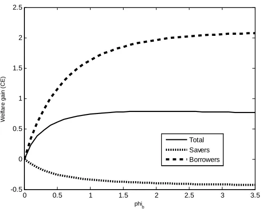
0 0.5 1 1.5 2 2.5 3 3.5 -0.5
0 0.5 1 1.5 2 2.5
phi
b
W
el
far
e gai
n (
CE)
[image:15.612.171.433.69.281.2]Total Savers Borrowers
Figure 2: Welfare gains from introducing the macroprudential rule, given monetary policy (di¤erent values of the reaction parameter for borrowing).
constraint relaxation, other indirect e¤ects may dominate. Notice thatk, the LTV ratio, is a parameter that strongly a¤ects the collateral constraint. A small change in this parameter can cause very large changes in borrowing that can be excessive. Higher LTVs lead to higher consumption levels, because borrowing constraints are always binding: the more borrowers are o¤ered, the more they take. But this in turn, as shown in Campbell and Hercowitz (2009), changes relative prices. In particular, higher consumption levels imply higher interest rates. This could lead to a situation of overindebtedness in the sense that high repayments could o¤set the positive e¤ects on constraint relaxation. In turn, higher interest rates imply higher returns on saving for savers. Smith (2009) shows that these results do not rely on the speci…c assumptions of Campbell and Hercowitz (2009); even in the simplest model with borrowers, savers, and collateral constraints, this e¤ect takes place.18
Figure 2 shows the welfare gains from introducing a macroprudential tool in the economy, given the Taylor rule. We use a steady-state value of the LTV of 0.9, as in Iacoviello (2005) and Iacoviello (2013). Therefore, we are in a region in which trade-o¤s should appear. Leaving …xed monetary policy, we present welfare for a continuum of values of the reaction parameters in the LTV rule, from a less to a more aggressive rule. The …gure is very informative because it shows welfare gains for each agent in the economy and for the aggregate. The conclusions we can obtain from the …gure are the following;
1 8
Using both policy measures at the same time is unambiguously welfare enhancing, as we can observe from the solid line. We can see that welfare increases by more, the larger the response of the LTV to credit growth is, but up to a point in which welfare stops increasing. The …gure also shows the trade-o¤ between borrowers and savers’ welfare, illustrated by the di¤erence between the two dashed lines. Borrowers’ welfare increases with the introduction of the macroprudential rule because tightening the collateral constraint avoids situations of overindebtedness in which debt repayments are a burden for them. Furthermore, borrowers can bene…t from more …nancial stability in the economy, as we will show later on. Notice that borrowers have a collateral constraint which is always binding and this does not allow them to make consumption smoothing. They do not have an Euler equation to smooth consumption as savers do. A more stable …nancial system smooths their consumption path thus mitigating the negative e¤ects of the collateral constraint. This welfare gain is at the expense of savers, who lose from having this measure in the economy, given that they are not …nancially constrained. However, the borrower´s welfare gain compensates the loss of the savers and globally, the measure is welfare increasing.
Next section performs an optimal policy analysis in order to assess which are the combination of values of the reaction parameters which would maximize welfare and make policy recommendations on this issue.
4
Optimal Policy Analysis
4.1 Optimal Parameters
In this section, we aim at …nding the optimal combination of policy parameters that maximizes welfare. For this purpose, we consider three di¤erent cases; a benchmark case in which there is only a monetary authority that acts in the traditional way, using the interest rate as an instrument. Then, we include a macroprudential authority that introduces an extra instrument, the LTV ratio. We study the interaction between the two authorities from two perspectives, when they act both from a coordinated and a non-coordinated way.
are two types of distortions: price rigidities and credit frictions. This creates con‡icts and trade-o¤s between borrowers and savers. Savers may prefer policies that reduce the price stickiness distortion. However, borrowers may prefer a scenario in which the pervasive e¤ect of the collateral constraint is softened. Borrowers operate in a second-best situation. They consume according to the borrowing con-straint as opposed to savers that follow an Euler equation for consumption. Borrowers cannot smooth consumption by themselves, but a more stable …nancial system would provide them a setting in which their consumption pattern is smoother. Therefore, in order to assess the optimality of policies, factors that help borrowers smooth their consumption should be included. Studies show that, in these kind of models, …nancial variables should be included in the loss function that the policy maker aims at minimizing.19
In the standard sticky-price model, the Taylor rule of the central bank is consistent with a loss function that includes the variability of in‡ation and output. In order to rationalize the Taylor rule of the macroprudential regulator, we follow Angelini et al. (2012) in which they assume that the loss function in the economy also contains …nancial variables, namely borrowing variability, as a proxy for …nancial stability. Then, there would be a loss function for the economy that would include not only the variability of output and in‡ation but also the variability of borrowing: L= 2+
y 2y+ 2b where
2; 2
y and b2 are the variances of in‡ation, output and borrowing. y 0, represents the relative weight
of the central bank to the stabilization of output.20
If the central bank and the macroprudential regulator coordinate, they would aim at jointly minimiz-ing the loss function each one with its own instrument. The problem becomes analogous to the Mundell’s assignment rule in which each arm of policy concentrates on a single task, addressing the issue it cares most about, and making coordination of policy trivial.21 Following this line of argument, we consider a case in which we jointly optimize the parameters of both rules.
However, Svensson (2012) argues that conducting monetary policy and …nancial-stability policy in an integrated way may be inappropriate, since monetary policy and …nancial-stability policy are distinct and separate policies with di¤erent objectives and di¤erent instruments. Tinbergen (1952) put forth what we now call the ‘Tinbergen principle,’ that policymakers need at least one independent policy
1 9
Andrés et al. (2013) …nd that optimal monetary policy may involve a trade-o¤ between the stabilization of in‡ation, output gap, consumption gap and the distribution of the collateral asset between constrained and unconstrained consumers.
2 0This loss function would be consistent with studies that make a second-order approximation of the utility of individuals
and …nd that it di¤ers from the standard case by including …nancial variables.
2 1
instrument for each policy objective. Since the policy interest rate is used by monetary policymakers to achieve the objective of price stability, at least one other instrument is required to achieve the additional objective of …nancial stability of macroprudential policy. Svenson (2012) suggests that monetary policy should be in charge of price stability while macroprudential policy needs to address …nancial stability. He argues that monetary policy should be conducted taking the macroprudential policy into account, and vice-versa, as in a Nash equilibrium rather than a coordinated equilibrium. Therefore, we study a second case in which the central bank and the macroprudential regulator play a non-coordinated game. The central bank would …nd the optimal parameters in its policy rule, taking the macroprudential regulator behavior as given. Similarly, the macroprudential authority would …nd the best response given monetary policy. The intersection of these two best responses would give us the Nash equilibrium.
In order to contribute to the discussion and evaluate the welfare gains of introducing macroprudential polices, we …rst compute the optimal parameters of the Taylor rule for monetary policy, assuming that there is no macroprudential regulator. Then, we compute the optimal monetary and macroprudential policies for the coordinated and the non-coordinated game.
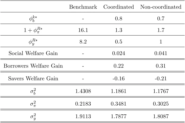
[image:18.612.128.484.436.673.2]Table 1 shows the optimal parameter values and the welfare gains in consumption equivalents, taking as a benchmark the situation without macroprudential policy. We also present the implied volatilities:
Table 1: Optimal Macroprudential and Monetary Policy mix
Benchmark Coordinated Non-coordinated
k
b - 0.8 0.7
1 + R 16.1 1.3 1.7
R
y 8.2 0.5 1
Social Welfare Gain - 0.024 0.041
Borrowers Welfare Gain - 0.22 0.31
Savers Welfare Gain - -0.16 -0.21
2
b 1.4308 1.1861 1.1767
2 0.2183 0.3481 0.3025
2
y 1.9113 1.7877 1.8087
As expected, when there does not exist a macroprudential regulator, the central bank needs to act in a very aggressive way, given that it only counts with a single instrument to minimize the loss function.22
We take this case as a benchmark, both for welfare and for macroeconomic and …nancial volatilities (presented in the …rst column).
The second column presents the case in which there is a macroprudential regulator that acts in a coordinated way with the central bank. We see that adding this extra instrument produces a welfare gain in the economy. In this case, monetary policy does not need to be as aggressive as in the benchmark case because it counts with the help of the macroprudential policy. However, as already pointed out, there is a trade-o¤ between borrowers and savers and, while borrowers are better-o¤, savers are not. Furthermore, if we compare the volatilities that this combination of policies generates, with respect to the benchmark case, we observe that the standard deviation of borrowing decreases, which is what makes borrower’s welfare increase. In terms of the macroeconomic volatilities, we see that the volatility of output decreases, but this comes at the expense of a higher in‡ation volatility.23 This higher in‡ation volatility contributes to decrease savers’welfare.
Nevertheless, if both authorities act in a non-coordinated way, social welfare gains are even higher. As Svensson (2012) argues, letting each regulator focusing on its own objective, leads to more e¤ective results in reducing volatilities. In this case, monetary policy acts in a more aggressive way, favoring the reduction of the volatility of in‡ation. The macroprudential authority reaction parameter does not need to be as high as in the previous case to obtain a lower standard deviation of borrowing. As usual, we also observe the same trade-o¤ between borrowers and savers.
4.2 Pareto-superior Outcomes
Results from optimal policy analysis show that trade-o¤s between the two agents appear. However, if the welfare gain that borrowers obtain is large enough, there could be room for Pareto-superior outcomes.
In order to do that, we apply the concept of Kaldor–Hicks e¢ ciency, also known as Kaldor–Hicks criterion24. Under this criterion, an outcome is considered more e¢ cient if a Pareto-superior outcome can be reached by arranging su¢ cient compensation from those that are made better-o¤ to those that are made worse-o¤ so that all would end up no worse-o¤ than before. The Kaldor–Hicks criterion does not require the compensation actually being paid, merely that the possibility for compensation exists, and thus need not leave each at least as well o¤.
that …nancial variables enter in the Taylor rule for the central bank. For further discussion on interactions between di¤erent rules, see Kannan et al. (2012) or Rubio and Carrasco-Gallego (2013).
2 3
This result is consistent with other studies on macroprudential policies. See for instance, Mendicino et al. (2013).
In our case, our measure for welfare presented in consumption equivalents is given by equations
(26)and(27). Since, there is a trade-o¤ between savers and borrowers, introducing the macroprudential policy, both in coordination and non-coordination with monetary policy, producesCEb >0andCEs<0.
Thus, a Kaldor-Hicks improvement to a obtain Pareto-superior outcome would be one in which:
CEb "b 0
and
CEs+"b = 0:
Then,
"b 1 exp (1 s) WsM P Ws : (28)
[image:20.612.60.571.492.653.2]That is, a system of transfers in which the borrowers would compensate the savers with at least the amount they are losing, so that they are at least indi¤erent between having or not the macroprudential policy. Then, the new outcome would be desirable for the society and there would be no agent that would lose with the introduction of the new policy. Then, if equation (28) holds with equality, the borrower compensates the saver with the exact welfare that she is losing. Then, in our case, after the compensations are made, the …nal result is the following:
Table 2: Optimal Macroprudential and Monetary Policy mix (Kaldor-Hicks Improvement)
Benchmark Coordinated Non-coordinated
k
b - 0.8 0.7
1 + R 16.1 1.3 1.7
R
y 8.2 0.5 1
Social Welfare Gain - 0.024 0.041
Borrowers Welfare Gain - 0.06 0.10
Savers Welfare Gain - 0 0
4.3 Impulse Responses
in the previous section. We compare the benchmark (no macroprudential policy) with the case in which monetary and macroprudential policies coexist, both in a coordinated and in a non-coordinated game. We consider a technology shock and a housing demand shock.
The discount factor for savers, s, is set to 0.99 so that the annual interest rate is 4% in steady state.
The discount factor for the borrowers is set to 0.98.25 The steady-state weight of housing in the utility function, j, is set to 0.1 in order for the ratio of housing wealth to GDP to be approximately 1.40 in the steady state, consistent with the US data. We set = 2, implying a value of the labor supply elasticity of 1.26 For the parameters controlling leverage, we setk
SS to 0.90, in line with the US data.27 The labor
income share for savers is set to 0.64, following the estimate in Iacoviello (2005). For the Taylor rule, we consider the optimized parameters found in the previous section. For we use 0.8, which also re‡ects a realistic degree of interest-rate smoothing.28
We assume that technology,At, follows an autoregressive process with0:9persistence and a normally
distributed shock. We also assume that the weight of housing on the utility function is equal to its value in the steady state plus a shock which follows an autoregressive process with 0:95 persistence.29 For the reactions parameter in the LTV rule, we use the optimized parameters both for the coordination and non-coordination with monetary policy. Table 3 presents a summary of the parameter values used:
2 5Lawrance (1991) estimated discount factors for poor consumers at between 0.95 and 0.98 at quarterly frequency. We
take the most conservative value.
2 6
Microeconomic estimates usually suggest values in the range of 0 and 0.5 (for males). Domeij and Flodén (2006) show that in the presence of borrowing constraints this estimates could have a downward bias of 50%.
2 7
See Iacoviello (2013).
2 8As in McCallum (2001). 2 9
Figure 3: Impulse responses to a technology shock. Optimized parameters.
Table 3: Parameter Values
s :99 Discount Factor for Savers b :98 Discount Factor for Borrowers
j :1 Weight of Housing in Utility Function
2 Parameter associated with labor elasticity k :9 Loan-to-value ratio
:64 Labor share for Savers X 1:2 Steady-state markup
:75 Probability of not changing prices
A :9 Technology persistence j :95 Housing demand shock persistence
:8 Interest-Rate-Smoothing Parameter in Taylor Rule
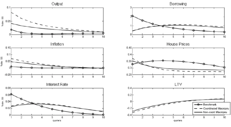
4.3.1 Technology Shock
Figure 3 presents impulse responses to a 1 percent shock to technology. Given the technology shock, output increases and in‡ation decreases.
Figure 4: Impulse responses to a housing demand shock. Optimized parameters.
Given the expansion in the economy, borrowing and housing demand increase, leading to an increase in house prices.
However, when the macroprudential rule interacts with monetary policy, the reaction of the interest rate is not as strong, given that the optimal parameters of the Taylor rule are lower. The LTV ratio decreases to cut credit because borrowing is growing following the boom. Therefore, when the macro-prudential rule is in place, borrowing does not increase as much as in the benchmark, and this mitigates the e¤ects of the boom.
Concerning the di¤erence between the coordinated and the non-coordinated case, the pattern of the impulse responses is very similar. Nevertheless, the non-coordinated case is always slightly closer to the benchmark. This is due to the fact that the reaction parameters in the Taylor rule are higher for the coordinated case and thus more similar to the benchmark.
4.3.2 Housing Demand Shock
In …gure 4, we see the e¤ects of a 25 percent housing demand shock. Given the increase in demand, house prices increase as well. This directly a¤ects the collateral constraint and borrowers are able to borrow more out of their housing collateral, which is worth more now. The wealth e¤ect permits them consume both more houses and consumption goods. The increase in house prices is, therefore, transmitted to the real economy and output increases.
The raise in output generates in‡ation and the Taylor rule responds with a higher interest rate. This is particularly true in the benchmark case in which monetary policy is more aggressive. On impact, this higher interest rate also dampens the increase in the price of the house, especially for the benchmark for the same reasons. Therefore, the initial shock is mitigated in the case in which monetary is the only policy in action.
When the macroprudential and the monetary policy interact, the LTV decreases to moderate the credit boom. This is the reason why, in this case, borrowing does not increase as much as in the benchmark. However, as we have seen, the increase in the interest rate is not as strong as in the benchmark and therefore the e¤ects on real output of this demand shock are more noticeable. In the case of this shock, the combination of the macroprudential and the monetary policies manage to control credit without moderating the real e¤ects of the boom.
As in the previous case, and for the same reasons, the non-coordinated situation is closer to the benchmark.
4.4 Financial and Macroeconomic Stability
Results from the optimal policy analysis have shown that the combination of macroprudential and mon-etary policies deliver a more stable …nancial and macroeconomic scenario. In order to show graphically these results, we plot an e¢ ciency frontier that includes the three objectives that the policy makers aim at minimizing: variability of output, variability of in‡ation and variability of borrowing.
Policy analysis is usually done through policy frontiers, also known as Taylor curves or e¢ ciency frontiers.30 This curve shows, given di¤erent parameters of the Taylor rule, the combination that delivers
the lower output and in‡ation variability. Therefore, a Taylor curve which is closer to the origin would be more e¢ cient. In order to include the objective of the macroprudential regulator, we present an extended Taylor curve in which we include the variability of borrowing, as a measure to capture …nancial stability.
Figure 5: Three dimensional e¢ ciency frontier.
We are aware that there is not a widely accepted de…nition of …nancial stability or systemic risk. Those are di¢ cult concepts to de…ne and to measure. Many de…nitions include the interactions between the …nancial and the real sector.31 In our model, we characterize the …nancial sector implicitly: borrowers take credits from savers and sign mortgages to buy houses, the asset of our model. Therefore, the …nancial system can be proxied by the amount of borrowing that takes place. Within this framework, we propose a measure for …nancial stability: a low variability of borrowing. In this sense, a lower variance of borrowing would imply a more stable …nancial system: if the variance of borrowing is lower, credit is smoother. A more stable …nancial system contributes to a lower systemic risk. Our model …ts this idea. Borrowers do not have an Euler equation that allows them to smooth their consumption, as savers do. If the variability of the borrowing is lower then borrowers can sign mortgages in a smoother way and also can achieve a more stable consumption. The …nancial sector will be more stable and also the real sector. The economy can bene…t from a more stable …nancial system and a lower systemic risk with a higher welfare, as we proved in previous sections. However, if the situation is the opposite and there is a high variability of borrowing, the …nancial system will be more unstable: with credit being more variable, consumption would also be more variable, the systemic risk will increase and, therefore, welfare will be lower.
the standard objectives of the central bank, while the third one would be the objective of the macro-prudential regulator. As in previous cases, we are comparing the macromacro-prudential (coordinated and non-coordinated) with the no macroprudential scenario (benchmark). Here, curves are preferable the lower (less borrowing variance) and closer to the in‡ation and output variance origin (less in‡ation and output variability) are. We see that when we take the three dimensions together, macroprudential and monetary policies interacting with each other manage to deliver a more stable scenario, which includes not only macroeconomic stability but also …nancial stability. These results represent a way to convey the …ndings in previous sections, that is, the introduction of the macroprudential policy is welfare enhancing because it is delivering a more stable system.
5
Concluding Remarks
In this paper, we analyze the impact of macroprudential and monetary policies on business cycles, welfare, and …nancial stability. In particular, we consider a macroprudential rule on the LTV ratio that responds to credit growth.
We compute the optimal parameters of the macroprudential and monetary rule both when monetary and macroprudential policies act in a coordinated and in a non-coordinated way. We …nd that in both cases, this interaction is welfare improving for the society, especially in the case of the non-coordinated game. However, there is a trade-o¤ between the agents of the model and savers lose from this new scenario. We …nd that by transfers à la Kaldor-Hicks, so that borrowers can compensate the saver’s welfare loss, a Pareto-superior outcome can be obtained.
From a positive perspective, we show the dynamics of the model under the optimal parameters that maximize welfare. We …nd that, given a positive technology or housing demand shock, the macropru-dential authority would decrease the LTV to moderate the credit boom. In this way, it can achieve its ultimate goal: …nancial stability.
Appendix
Main Equations
1
Cs;t
= sEt
Rt
t+1Cs;t+1
; (29)
wts= (Ns;t) 1Cs;t; (30)
j Hs;t
= 1
Cs;t
qt sEt
1
Cs;t+1
qt+1: (31)
1
Cb;t
= bEt
Rt
t+1Cb;t+1
+ tRt; (32)
wb;t= (Nb;t) 1Cb;t; (33)
j Hb;t
= 1
Cb;t
qt bEt
1
Cb;t+1
qt+1 btktEt(qt+1 t+1): (34)
Et
Rt
t+1
bt=ktEtqt+1Hb;t; (35)
Cb;t+qtHb;t+
Rt 1bt 1
t
=qtHb;t 1+wb;tLb;t+bt; (36)
ws;t=
1
Xt
Yt
Ns;t
; (37)
wb;t=
1
Xt
(1 ) Yt
Nb;t
; (38)
bt= Etbt+1 bxt+u t (39)
Ws;t Et
1
X m
s logCs;t+m+jlogHs;t+m
(Ns;t+m)
Wb;t Et
1
X
m=0
m
b logCb;t+m+jlogHb;t+m
(Nb;t+m)
; (41)
Wt= (1 s)Ws;t+ (1 b)Wb;t: (42)
References
[1] Abraham, J.,Pavlov,A.,Wachter,S., (2008), "Explaining the United States’ uniquely bad Housing Market", Wharton Real Estate Review 12 (1) ,24–41.
[2] Agénor, P., Pereira da Silva, L., (2011), Macroeconomic Stability, Financial Stability, and Monetary Policy Rules, Ferdi Working Paper, 29
[3] Allen, F. and Carletti, E. (2013) ‘Systemic risk from real estate and macro-prudential regulation’, Int. J. Banking, Accounting and Finance, Vol. 5, Nos. 1/2, pp.28–48
[4] Almeida, H., Campello, M. and Liu, C. (2006), ‘The …nancial accelerator: evidence from interna-tional housing markets’, Review of Finance 10, pp. 1-32.
[5] Andres, J., Arce, O., Thomas, C., (2013), “Banking Competition, Collateral Constraints, and Optimal Monetary Policy,” Journal of Money, Credit and Banking - Supplement to Vol 45, No 2
[6] Angelini, P., Neri, S., Panetta, F., (2012), Monetary and macroprudential policies, Working Paper Series 1449, European Central Bank.
[7] Antipa, P., Mengus, E. and Mojon, B. (2010) Would macroprudential policy have prevented the Great Recession? Mimeo, Banque de France
[8] Ascari, G., Ropele, T., (2009), Disin‡ation in a DSGE Perspective: Sacri…ce Ratio or Welfare Gain Ratio?, Kiel Institute for the World Economy Working Paper, 1499
[9] Bean, C. (2009) The great moderation, the great panic and the great contraction. Schumpeter Lecture delivered at the Annual Congress of the European Economic Association, Barcelona, 25 August 2009.
[11] Beau, D., Clerc, L., Mojon, B., (2012), Macro-prudential policy and the conduct of monetary policy, mimeo, Bank of France
[12] Benigno, P., Woodford, M., (2008), Linear-Quadratic Approximation of Optimal Policy Problems, mimeo
[13] Borio, C., Shim, I., (2007), What can (macro-) policy do to support monetary policy?, BIS Working Paper, 242
[14] Brázdik, F., Hlaváµcek, M., Maršal, A., (2012), "Survey of Research on Financial Sector Modeling within DSGE Models: What Central Banks Can Learn from it", Czech Journal of Economics and Finance , 62 (3)
[15] Campbell, J., Hercowitz, Z., (2009), "Welfare Implications of the Transition to High Household Debt", Journal of Monetary Economics, 56 (1), 1-16
[16] Caruana, J., (2010a), Macroprudential policy: what we have learned and where we are going, Keynote speech at the Second Financial Stability Conference of the International Journal of Central Banking, Bank of Spain
[17] Caruana, J., (2010b). The Challenge of Taking Macroprudential Decisions: Who Will Press Which Button(s)?, in Macroprudential Regulatory Policies. The New Road to Financial Stability? Edited by Stijn Claessens, Douglas Evano¤, George Kaufman and Laura Kodres. World Scienti…c, New Jersey
[18] Clement, P. (2010). The term “macroprudential”: origins and evolution, BIS Quarterly Review
[19] Committee on the Global Financial System (2010a), The role of margin requirements and haircuts in procyclicality, CGFS Papers, 36
[20] Committee on the Global Financial System (2010b), Macroprudential instruments and frameworks: A stocktaking of issues and experiences, CGFS Papers, 38
[21] Committee on the Global Financial System (2012), Operationalising the selection and application of macroprudential instruments, CGFS Papers, 48
[23] Domeij, D., Flodén, M., (2006) "The Labor-Supply Elasticity and Borrowing Constraints: Why Estimates are Biased." Review of Economic Dynamics, 9, 242-262
[24] Duca, J.V., Muellbauer, J., Murphy, A., (2011), Shifting Credit Standards and the Boom and Bust in US House Prices, SERC Discussion Paper 76.
[25] Financial Stability Board, Bank for International Settlements and International Monetary Fund (2009). Guidance to assess the systemic importance of …nancial institutions, markets and instru-ments: initial considerations
[26] Financial Stability Board, Bank for International Settlements and International Monetary Fund (2011). Macroprudential policy tools and frameworks. Update to G20 Finance Ministers and Central Bank Governors
[27] Funke, M., Paetz, M., (2012), A DSGE-Based Assessment of Nonlinear Loan-to-Value Policies: Evidence from Hong Kong, BOFIT Discussion Paper No. 11/2012
[28] Galati, G. and Moessner, R. (2013). Macroprudential Policy – A Literature Review. Journal of Economic Surveys Vol. 27, No. 5, pp. 846–878
[29] Galvão, A.B., Owyang, M. T., (2013), Measuring Macro-Financial Conditions using a Factor-Augmented Smooth-Transition Vector Autoregression, Mimeo
[30] Gelain, P., Lansing, K., Mendicino, C., (2013), "House Prices, Credit Growth, and Excess Volatility: Implications for Monetary and Macroprudential Policy", International Journal of Central Banking, 9 (2)
[31] Gerali, A., Neri, S., Sessa, S. and Signoretti, F. (2010) Credit and banking in a DSGE model of the euro area. Bank of Italy Economic Working Papers No. 740.
[32] Goodhart, C.A.E. (2004) Some new directions for …nancial stability? The Per Jacobsson Lecture, Zürich
[33] Gruss, B., Sgherri, S., (20090, The Volatility Costs of Procyclical Lending Standards: An Assessment Using a DSGE Model, IMF Working Paper, 09/35.
[35] Iacoviello, M., (2005) "House Prices, Borrowing Constraints and Monetary Policy in the Business Cycle." American Economic Review, 95 (3), 739-764
[36] Iacoviello, M., (2011), Financial Business Cycles, Mimeo, Federal Reserve Board
[37] Iacoviello, M. , Neri, S., (2010), “Housing Market Spillovers: Evidence from an Estimated DSGE Model,” American Economic Journal: Macroeconomics, 2, 125–164.
[38] IMF, Monetary and Capital Markets Division, (2011), Macroprudential Policy: An Organizing Framework, mimeo, IMF
[39] Jeanne, O., Korinek, A., (2011), Macroprudential Regulation versus mopping after the Crash, mimeo
[40] Kannan, P., Rabanal, P., Scott, A., (2012), "Monetary and Macroprudential Policy Rules in a Model with House Price Booms", The B.E. Journal of Macroeconomics, Contributions, 12 (1)
[41] Lawrance, E., (1991), "Poverty and the Rate of Time Preference: Evidence from Panel Data", The Journal of Political Economy, 99 (1), 54-77
[42] Lim, C.H., Columba, F., Costa, A., Kongsamut, P., Otani, A., Saiyid, M., Wezel, T., Wu, X., (2011), Macroprudential policy: what instruments and how to use them? Lessons from country experiences, IMF Working Paper 11/238.
[43] McCallum, B., (2001), "Should Monetary Policy Respond Strongly To Output Gaps?," American Economic Review, 91(2), 258-262
[44] McCauley, R., (2009), Macroprudential policy in emerging markets, Presentation at the Central Bank of Nigeria’s 50th Anniversary International Conference on Central banking, …nancial system stability and growth, 4–9 May.
[45] Mendicino, C., Pescatori, A., (2007), Credit Frictions, Housing Prices and Optimal Monetary Policy Rules, mimeo
[46] Monacelli, T., (2006), "Optimal Monetary Policy with Collateralized Household Debt and Borrowing Constraint," in conference proceedings "Monetary Policy and Asset Prices" edited by J. Campbell.
[48] N’Diaye, P., (2009), Countercyclical macro prudential policies in a supporting role to monetary policy, IMF Working Paper
[49] Posner, R. (2007), Economic Analysis of Law (Seventh ed.), Austin, TX: Wolters Kluwer.
[50] Recommendation of the European Systemic Risk Board (2013) O¢ cial Journal of the European Union of 15.6.2013, on intermediate objectives and instruments of macro-prudential policy.
[51] Reinhart, C., Rogo¤, K., (2009), "This Time is Di¤erent: Eight Centuries of Financial Folly", Princeton University Press
[52] Rubio, M. and Carrasco-Galllego, J. (2013), Macroprudential Measures, Housing Markets, and Monetary Policy, Moneda y Crédito
[53] Saurina, J., (2009a), Dynamic provisioning. The experience of Spain, in Crisis Response. Public Policy for the Private Sector, note 7, World Bank
[54] Saurina, J., (2009b), “Loan loss provisions in Spain. A working macroprudential tool”, Revista de Estabilidad Financiera, 17, Bank of Spain, 11–26.
[55] Schmitt-Grohe, S., Uribe, M., (2004), "Solving Dynamic General Equilibrium Models Using a Second-Order Approximation to the Policy Function," Journal of Economic Dynamics and Con-trol, 28, 755-775
[56] Smith A., (2009), Comment on "Welfare Implications of the Transition to High Household Debt" by Campbell J., Hercowitz, Z., Journal of Monetary Economics, 56 (1)
[57] Suh, H., (2011), Simple, Implementable Optimal Macroprudential Policy, Mimeo, Indiana University
[58] Tinbergen, J. (1952) On the Theory of Economic Policy. Amsterdam: North Holland Publishing Company.