On Continuous Limiting Behaviour for the q(n) Binomial Distribution with q(n)→1 as n→∞

On Continuous Limiting Behaviour for the

 

q n

-Binomial Distribution with

 

1

q n



as

n

 

Malvina Vamvakari

Department of Informatics and Telematics, Harokopio University of Athens, Athens, Greece Email: [email protected]

Received September 28, 2012; revised October 28, 2012; accepted November 5, 2012

ABSTRACT

Recently, Kyriakoussis and Vamvakari [1] have established a q-analogue of the Stirling type for q-constant which have

lead them to the proof of the pointwise convergence of the q-binomial distribution to a Stieltjes-Wigert continuous

dis-tribution. In the present article, assuming q n

 

a sequence of n with q n

 

1 as n , the study of the affect of

this assumption to the -analogue of the Stirling type and to the asymptotic behaviour of the -Binomial dis-tribution is presented. Specifically, a analogue of the Stirling type is provided which leads to the proof of de-formed Gaussian limiting behaviour for the

 

 

q n q n

 

 

q n

 

q n -Binomial distribution. Further, figures using the program MAPLE

are presented, indicating the accuracy of the established distribution convergence even for moderate values of n.

Keywords: Stirling Formula; -Factorial Number of Order n; Saddle Point Method; -Binomial

Distribution; Pointwise Convergence; Gauss Distribution

 

q n q n

 

1. Introduction and Preliminaries

In last years, many authors have studied -analogues of the binomial distribution (see among others [2-4]). Spe- cifically, Kemp and Kemp [3] defined a -analogue of the binomial distribution with probability function in the form

q

q

 







1

2 1

1

1

0,1, , , X

x n

x j

j q

f x P X x

n

q q

x

x n

 

 

  _ 

  

 

 

_{ } 

  







, (1)

where  0, 0 q 1, by replacing the loglinear re- lationship for the Bernoulli probabilities in Poissonian random sampling with loglinear odds relationship. Also, Kemp [4] defined (1) as a steady state distribution of birth-abort-death process.

Futhermore, Charalambides [2] considering a sequen- ce of independent Bernoulli trials and assuming that the odds of success at the ith trial given by

1

π i , 1, 2, ,0 1,0

i q i q



       ,

is a geometrically decreasing sequence with rate q, de-

rived that the probability function of the number X of

successes up to n-trail is the q-analogue of the binomial

distribution with p.f. given by Equation (1).

For q constant, the q-binomial distribution has finite

mean and variance when .Thus, the asymptotic normality in the sense of the DeMoivre-Laplace classical limit theorem did not conclude, as in the case of ordinary hypergeometric series discrete distributions. Also, asym- ptotic methods—central or/and local limit theorems—are not applied as in Bender [5], Canfield [6], Flajolet and Soria [7], Odlyzko [8] et al.

n 

Recently, Kyriakoussis and Vamvakari [1], for q con-

stant, established a limit theorem for the q-binomial dis-

tribution by a pointwise convergence in a q-analogue

sense of the DeMoivre-Laplace classical limit theorem. Specifically, the pointwise convergence of the q-bino-

mial distribution to a Stieltjes-Wigert continuous distri- bution was proved. In detail, transferred from the random variable X of the q-binomial distribution (1) to the

equal-distributed deformed random variable

 

₁ q, then, for the q-binomial distribution was app-

roximated by a deformed standardized continuous Stieltjes-Wigert distribution as follows

Y X

,

 

 





 





 





 

1 2

1 8 1

1 2

1 2 1 2 1

3 2 1

1 2 1

2 3 2 1

log

2π

1

1 log

exp , 0,

2log

X

q q

q

q q

q

q q

f x

x

q q q

x

q q q

x q

 

  

 

 



  

 

_   _

 

   

 _   _

 _{ }

   

 

 

 

 

(2)

where   n,n0,1, 2, such that

n n q



 _  _with

constant and q

0 a 1  and _q2 the mean value

and variance of the random variable respectively. To obtain the above pointwise convergence (2), a q-

analogue of the well known Stirling formula for the factorial has been provided.

,

Y

n

 

n!

In statistical mechanics and in computer science such as in probabilistic and approximation algorithms, appli- cations of the -binomial distribution involve sequences of independent Bernoulli trials where in the geo- metrically decreasing odds of success at the th trial, the rate is considered to be a sequence of with

as n . In this work, under this con- sideration, a question arises. How this assumption affects the continuous limiting behaviour of this q-binomial

distribution?

q



i q



 

1 n

q q n  

The answer to this question is given in this manuscript by establishing a deformed Gaussian limiting behaviour for the -Binomial distribution is proved. The proofs are concentrated on the study of the sequence

 

q n

 

q n and the parameters of the considered distribution

as sequences of . Further, figures using the program MAPLE are presented, indicating the accuracy of the established distribution convergence even for moderate values of .

n

n

2. Main Results

2.1. An Asymptotic Expansion of the q(n)-Factorial Number of Order n with

as

 

1

q n  n 

To initiate our study we need to derive an asymptotic expansion for n  of the q-factorial number of order

n

 

     





 





1

! 1 2

; 1

,

1 1

q q q q

k n

n

n n

k

n n

q q q

q q



 

 

 





(3)

where qq n

 

with q n

 

1 as n  and

 

1

1 t

q

q t

q

 

 , the q-number t.

The derived estimate for the -factorial numbers of order , is based on the analysis of the -Exponential function

q

n q









 





 









2

0

2

0

1 1

1 1

;

!

1 1 n

n n q

n _n

n

n

n _q

j

j

q q

E q x x

q q

q x n

q xq  

    

       

 

 



 



  







(4)

which is the ordinary generating function (g.f.) of the

numbers

 

2

, 0,1, 2,

!

n

q

q n n

     

 .

Rewriting Eq





1q



x



as follows

 

exp





,

q

E x  g x





(5)

where

 











1



1

log 1 1 j ,

j

g x q x q



 





  (6)

because of the large dominant singularities of the gene- rating function Eq

 

x , a well suited method for analyz-

ing this is the saddle point method.

Using an approach of the saddle point method inspired from [9-12] and [1], the following theorem gives an asymptotic for the q n

 

-factorial number of order n.

Theorem 1. The q-factorial numbers of order

,

n

 

n_q!, where

A) qq n

 

with q n

 

1 as n

n



 

 

and q n   1

or

B)

 

with

 

n

 

1

qq n q n o

have the following asymptotic expansion for n 

 

 

 





 

 

  















1 2 2

1 2 2

1 1 2 1

! 2π

exp

1 1 1

n

q

n

N

N _k

n n

k k

n q

g r rg r r g r r

S r q q O q q

     

  

 



   

 _  _

  

      

  







(7)

where is a positive integer, is the real solution of the equation

N r

   

 

 









 

 

 

 









 

 

2

2 , 1 2 1 2

1

2 1 1

2 1 2

1

2 !

1 2

, , ,

π

2 1 i

1 2

2, k

k

k

k j k

j

k k

k k

k

r

S r

k

j k

B r r

rg r

g r r

g r k k r

S k r g  r



 





 



 





 



 

  





 

    

    

 _{ } _

  

 



   

 







2



(8)

with Bk j,



1, ,k



,j

1

 the partial Bell polynomials,

the Stirling numbers of the second kind and .



S k

2

i  

Proof. We shall study the asymptotic behaviour of the

-factorial numbers of order ,

q n

 

n_q!, by expressing

them via Cauchy’s integral formula that gives the coefficients of a power series:

 



 



2

1 exp 1

d ! 2π

n

n x r q

g x q

x

n i x

     

 





(9)

where the contour of integration is taken to be a circle of radius . This integral will be estimated with the saddle point method. The saddle point is defined by the equation r

 

1

xg x n . It turns out that it is convenient to switch

to polar coordinates, setting ei

xr . Then the original

integral becomes

 



 



 

 

2

π π

exp

! 2π

exp e d .

n

n q

i

g r q

n r

g r  g r in 

     





 





_   _

(10)

In accordance with the saddle point method principles, we choose the radius to be the solution of r

 

rg r n. Setting G

 

 g r

 

ei g r

 

in 0

with a Maclaurin series expansion about   we have

 

2 2

   

1 !

k k

k

G r

k



   

 

 

  





(11)

where

 

 



2



1 2

 

1₂

1

,

2 rg r r g r g r

_    _   _{ }  _

   (12)

and

 

 

 

 

 

 





2 1 2 1

0

2 1

2 1 e

,

1 2

k

k i

k k

rg r

g r

g r r

g r k k r

 





 

 



 _{ }

    

 _{ } _

  

 



   (13)

where

 2

 

2

 

0 0

d

e e

d k

k i i

g r  g r 



 

 

 

    

  .

The absence of a linear term in  indicates a saddle point. The function eG 

is unimodal with its peak at 0

 .

An estimation of the -factorial numbers of order q

 

,

n n !

q with defined by conditions (A) or (B) should naturally proceed by isolating separately small portions of the contour (corresponding to

q

x near the

real axis) as follows.

A) For qq n

 

with q n

 

n 

 

1 we set

 

 

1

2π

2

1

exp d ,

2π

1 _{exp d ,}

2π

I G

I G

 

 

 

 





 _ _

 _ _





(14)

and choose  such that the following conditions are true (see [12]):

C1) _n2_{ }, that is _{ n}1 2

C2) _n3_0, that is _{ n}1 3_,

where “ ” means “much smaller than”. A suitable choice for



 is _n3 8_.

As eG  _{decreases in}

 

_{,π ,}

   

eG _ eG , _{ }2π_. ₍₁₅₎ We will show in the sequel that from C1) and C2) it follows that eG 

is exponentially small, being domi- nated by a term of the form eO n

 

1 4 .

Indeed we have

 

1



 

2

 



2

2

G    rg r r g r  or

 

1



 

2

 



_.

2

G    rg r r g r n3 4 (16)

But

 

2

 





1

1

1 log

n

rg r r g r q

q  

    

or

 

2

  





1 2



1

1

1 . log

n n

q

rg r r g r q q

q

 





      (17)

For qq n

 

with q n

 

n 

 

1 we get

 

1 1 4 _.

2 G  O_ n _

  (18)

From which we find that

 

 

11 4

2

2 e e . (19)

n G

I O   O_  _

Thus, by C1),  has been taken large enough so that the central integral I1 “captures” most of the contri-

bution, while the remainder integral I2 is exponentially

small by (19).

We now turn to the precise evaluation of the central integral I1. We have

 

 

 

1 ₂ 1 2

2 2

1

1 1

π

( )

exp d

! k

k k

I

rg r r g r

r k



      







    

 

 

 _  _











 

(20)

where

 

 



2



1 2

1

.

2 rg r r g r 

 _{ } 

_  _

 

 (21)

Note that   as n , since

 

 





 

 

1 2

3 8 2

1 2

1 8 1 8

1 2

1 ₁

2

n rg r r g r

rg r

n

g r

  _{ } 

 _  _

 

      _  _ _ 

  

 



, Cn

where C a positive constant.

B) For qq n

 

with q n

 

n o

 

1 we set

 

 

3

2π

4

1 _{exp d ,}

2π 1

exp d ,

2π

n

n

I r G

I r G

 

 

   

 

 _

 _ _

 _{ }







(22)

and choose  such that the conditions C1) and C2) are true. We suitably select _{ n}3 8_.

As eG  _{decreases in}

 

_{,π ,}

  _e   _{, 2π .}

G G

e        (23)

We will now show that eG  _{is dominated by a term} of the form . Indeed, form C1), C2), 16) and 17) it follows that

 

1 O

 









3 4 1

1

exp exp 1 .

2 log

n

G

q

 



 

 _  _

 q n  (24)

From which we get

 





 

3 4

2 1

1 1 1 2 log

4 e e . (25)

n

q n G

n n q

I O r  O q

 

 

 _ _

 

 

 

Thus, for with the integral

4

 

qq n q n

 

no

 

1

I is negligibly small. We now turn to the precise

evaluation of the central integral I3. Since

 

 

 

 

 

 

3 4

2 1

3

1 1 1 2 log

1

exp d

2π

1 _{exp d}

2π 1

exp d

2π 1

exp d

2π

1 _{exp d}

2π

2 e

n

n

n

n

n

n

q n

n q

I r G

r G

r G

r G

r G

O q

 





 

 

 

 

 

 

 

  

 _

  

  

 

 _ _

 _{ }

 _ _

 _{ }

 _ _

 

 



 

 















we have

 

 

   

3 ₂ 1 2

2 2

1

1

π

exp d .

! n

k

k k

r I

rg r r g r

r k



   



 







    

 

 

   

 









(26)

We now unifiable proceed our proof for both condi- tions A) and B) and working analogously as in Ky- riakoussis and Vamvakari [1] we get our final estimation (7).

In the previous theorem due to saddle point method principles, we have chosen the radius r of the derived

asymptotic expansion (7) to be the solution of

 

rg r n. By solving this saddle point equation we get

that

 

1 1q

rq n

and

 

2

 

 

1

1 1

1

. log

n q

q

g r r g r n q

q

 



   

So, by substituting these to our estimation (7) the following corollary is proved.

Corollary 1. The q-factorial numbers of order

 

, !

q

n n , where

A) qq n

 

with q n

 

1 as n

 

n

 

 and q n   1

or

B)

 

with

 

n

 

1

qq n q n o

have the following asymptotic expansion for n 

 













 





















1 2

1 2 1

1 2 2 2

1

1

1

2π 1

!

log

1 1

1 1

q

n

n n

q n

n j j

q n

q q

q q n

O q q

q q



 

  _

  

 



 

  

 



.

2.2. Deformed Gaussian Limiting Behaviour for the q(n)-Binomial Distributions with

as

 

1

q n  n 

Transferred from the random variable X of the q-

binomial distribution (1) to the equal-distributed de- formed random variable

 

_1q, the mean value and variance of the random variable Y , say

Y  X

q

 and 2

q



respectively, are given by the next relations

 

₁ 1

q nq _qn

 

 



 (28)

and

  









 







 



2 2 1 2 2 2 2 1 ₁ 1 1 1 1 ₁ q q

q _{n n}

q q

n _n

n n

q q q

n n q _q        _    _        _ (29)

(see Kyriakoussis and Vamvakari [1]). Using the standardized r.v.

 

1q q

q X Z    

with q and q given in (28) and (29), the -analo- gue Stirling asymptotic formula (27) and inspired by [1], the following theorem explores the continuous limiting behaviour of the -binomial distribution with

as n .

q

 

q n

 

 

q n 1

Theorem 2. Let the p.f. of the q-binomial distribution be of the form

 

₂



₁



1

1

1 , 0,1,

x n x j X j q n , ,

f x q q x

x  

    _       _{ }  

 



 n

where   n,n0,1, 2, such that   n , as . Then, for

n 

A)

 

with

 

n

 

1

qq n q n  



or

B)

 

with

 

1 as and

 

n

 

1

qq n q n  n  q n o

with 0 1 constant

n

q  a

 _  _{ }

and n

the q n

 

,

  by a deformed standardized Gauss distribution -binomial distribution is approximated, for as follows n

 





 





 

1 2 1 1 2 2 1 1 2 1 log 2π 1

exp , 0.

2 _log X q q q q q q f x x x q         _    _  _    _ 

Proof. Using the q-analogue of Stirling type (27), for

 

qq n with q n

 

1 and q n

 

n 

 

1 or

 

 

1

q n no , the q-binomial distribution (1), is app-

roximated by

 





























 

1 2 1 1 2 1 1 1 2 1 2 1 1 log 1 2π 1 1 1 . 1 x n X x x j j x j x n q j q q f x q q q q

q q x

        _         





(31)

Let the random variable

 

1 1 ₁

1 X q q X q    

 and the q-

standardized r.v.

 

1q q q

X

Z 

 

 with q and q given by (28) and (29) respectively, then all the fo- llowing listed estimations are easily derived

 

1 1 ,

q q q

q

x   z



 

 _ 

  (32)



1 ₁



q ₁

x

q q

q q   z



 _  _ _{ } _{ 1,}

 

  (33)



1



1

1

log 1 1 1 ,

log

q q

q

x q z

q             _  _  _{ }    

 (34)

 

 





1 1 1 1

exp log 1 1 1

log log 1 x q q x q q q q q q x q z q z                    _{ }  _ _{ }           _  _  

  (35)

Also, the estimation of the next product

 _       (30)

















1 1 1 1 1 1 1 1 1

1 1 1

exp log 1 1 1 ,

x j j q j q j q q j q j q

q q q

q q z q

q z q

                           _   _  _{ }              _   _  _{ }  _{   }  







(36)

























1 1 2 1 2 2

log 1 1 1

1 _{log 1 1}

2 log

1 1

1 1 1

1

log 1 1 1

2 1 log 2 q j q j q q q q q q q q q q q q q q q q

q z q

q z q q z Li q z q z q z q                               _   _  _{ }          _  _  _           _ _   _{ }   _{ }    _{   }                _   _  _      







  





1 log ,

1 1 q 1

q q

O q

q   z

         _{ }     _  _   (37)

where Li2 the dilogarithmic function and 2 the Ber-

noulli number of order 2.

Moreover, working similarly for the sum appearing in the product



1





1

1 1

1 j exp log 1 j

n n j j q q                









(38)

the next estimation is obtained





 





 

2 1 1 1 2 1 2 1

log 1 log

2log

1_{log 1}

1 2 log . 2 1 j n n j n n n n n n q q Li q O    _    _             _      



 (39)

Applying all the previous the estimations (32)-(39) to the approximation (31), carrying out all the necessary manipulations and for n , by both conditions A) and B), we derive our final asymptotic (30). 

Remark 2. A realization of the sequence

considered in the above theorem 1A) is

 

, 0,1, 2,

q n n 

 

1 ,0

q n

n

 _

   1 with

 

n exp

 

.

q n  

Remark 3. Possible realizations of the sequence

considered in the above theorem 2B) are among others the next two ones

 

, 0,1, 2,

q n n 

 

1 1

 

or

 

1 1,0

ln c

q n q n c

n n 1.

     

Corollary 2 Let the random variable X with p.f. that

of the q n

 

n

-binomial distribution as in Theorem 2. Then for   the following approximation holds







1



 

1 1

,

2 2

0 ,

b a

P a X b Erf u Erf u

a b        (40) where













1 1 2 1 1 2 2 log q q a q a u q q      

 (41)

with

 

 

2

0

2 t_{exp d}

Erf t  x x





the Gauss error func-

tion.

Proof. Using the approximation (2) and the classical

continuity correction we have that





 









 





 

, 1 2 1 1 2

1 1 2

2 2 1 1 2 1 log 2π 1

exp d .

2 _log

x a b b a q q q q q

P a X b P X x

q x x q                _{  }   _{ }   _ _{  }    _{ }   





(42)

Setting

 

1q q

q x z    

the approximation (42) becomes





 









 

   





1 1 , 1 1 2 _{1 2} 1

2 1 2

1 2 ₁ 1 2

log 2π

1

exp d .

2 _log q q q q q q

x a b

q q

b

q a

q

P a X b P X x

q z z q                _       _{ }   _{ }   _ _{  }    _{ }   





(43)

Carrying out all the necessary manipulations, we get the final approximation (40). 

3. Figures Using Maple

In this section, we present a computer realization of app- roximation (30), by providing figures using the computer program MAPLE and the -series package developed by F. Garvan [13] which indicate good convergence even

for moderate values of n. Analytically, for the random

variable X, we give the Figures 1 and 2 realizing

Theorem 2(A), by demonstrating with diamond blue points the exact probability

 





Prob 1 1 ,

2 2

0,1, 2, , , X

f x P X x x X x

x n

 

   _     _

 

 

(44)

and with diamond green points the continuous pro- bability approximation

 



1



 

1 1

Prob

2 2

1 1

,

2 2

0 q n

x x

b x x X x

Erf u Erf u

x n



 

 _     _

 

 

 

(45)

with ux and ux1 given by Equation (41), for

 

 







 

 

1



1 ,

exp 1 1 exp 1 2exp 1 n n

n

q q n

n

q q

 

  

    

and n50,100.

Note that similar good convergence even for moderate values of n have been implemented for Theorem 2B).

The procedure in MAPLE which realizes the exact probability (44) and its approximation (45) for given and theta for both Theorem 2A) and 2B), is avai-

lable under request. ,

n q

4. Concluding Remarks

In this article, a deformed Gaussian limiting behaviour

0.14

0.12

0.1

0.08

0.06

0.04

0.02

0

[image:7.595.305.536.80.303.2]

10 20 30 40 50 t

Figure 1. Sketch of exact probability (44) by blue diamond points and probability approximation (45) by green dia- mond points, for n = 50.

0.1

0.08

0.06

0.04

0.02

0

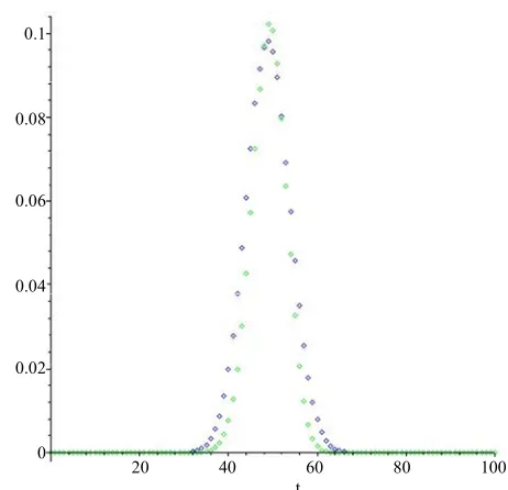
20 40 60 80 100 t

Figure 2. Sketch of exact probability (44) by blue diamond points and probability approximation (45) by green dia- mond points, for n = 100.

for the q n

 

-Binomial distribution has been established.

The proofs have been concentrated on the study of the sequence q n

 

and the parameters of the considered

distributions as sequences of Further, figures using the program MAPLE have been presented, indicating the accuracy of the established distribution convergence even for moderate values of n.

.

n

5. Acknowledgements

The author would like to thank Professor A. Kyriakoussis for his helpful comments and suggestions.

REFERENCES

[1] A. Kyriakoussis and M. G. Vamvakari, “On a q-Analogue of the Stirling Formula and a Continuous Limiting Be-haviour of the q-Binomial Distribution-Numerical Calcu-lations,” Methodology and Computing in Applied Prob-ability, 2011, pp. 1-27.

[2] Ch. A. Charalambides, “Discrete q-Distributions on Ber-noulli Trials with a Geometrically Varying Success Probability,” The Journal of Statistical Planning and In-ference, Vol. 140, No. 9, 2010, pp. 2355-2383.

[3] A. W. Kemp and C. D. Kemp, “Welson’s Dice Data Re-visited,” The American Statistician, Vol. 45, No. 3, 1991, pp. 216-222.

[4] A. W. Kemp, “Steady-State Markov Chain Models for Certain q-Confluent Hypergeometric Distributions,” Jour- nal of Statistical Planning and Inference, Vol. 135, No. 1, 2005, pp. 107-120. doi:10.1016/j.jspi.2005.02.009 [5] E. A. Bender, “Central and Local Limit Theorem Applied

[image:7.595.59.287.480.698.2]

doi:10.1016/0097-3165(73)90038-1

[6] E. R. Canfield, “Central and Local Limit Theorems for the Coefficients of Polynomials of Binomial Type,” Jour- nal of Combinatorial Theory, Series A, Vol. 23, No. 3, 1977, pp. 275-290.

doi:10.1016/0097-3165(77)90019-X

[7] P. Flajolet and M. Soria, “Gaussian Limiting Distribu-tions for the Number of Components in Combinatorial Structures,” Journal of Combinatorial Theory Series A, Vol. 53, No. 2, 1990, pp. 165-182.

doi:10.1016/0097-3165(90)90056-3

[8] A. M. Odlyzko, “Handbook of Combinatorics,” In: R. L. Graham, M. Grötschel and L. Lovász, Eds., Asymptotic Enumeration Methods, Elsevier Science Publishers, Am-sterdam, 1995, pp. 1063-1229.

[9] L. M. Kirousis, Y. C. Stamatiou and M. Vamvakari, “Upper Bounds and Asymptotics for the q-Binomial Co-efficients,” Studies in Applied Mathematics, Vol. 107, No.

1, 2001, pp. 43-62. doi:10.1111/1467-9590.1071177 [10] A. Kyriakoussis and M. Vamvakari, “On Asymptotics for

the Signless Noncentral q-Stirling Numbers of the First Kind,” Studies in Applied Mathematics,Vol. 117, No. 3, 2006, pp. 191-213.

doi:10.1111/j.1467-9590.2006.00352.x

[11] Ch. A. Charalambides and A. Kyriakoussis, “An Asymp- totic Formula for the Exponential Polynomials and a Central Limit Theorem for Their Coefficients,” Discrete Mathematics, Vol. 54, No. 3, 1985, pp. 259-270. doi:10.1016/0012-365X(85)90110-4

[12] P. Flajolet and R. Sedgewick, “Analytic Combinatorics, Chapter V: Application of Rational and Meromorphic Asymptotics, Chapter VIII: Saddle Point Asymptotics,” Cambridge University Press, Cambridge, 2009.