The Ascendency of Numerical Methods in Lens Design
1 2
Donald C. Dilworth 3
Optical Systems Design, Inc.; Correspondence: [email protected] 4
Tel.: 207-633-3711 5
Received: date; Accepted: date; Published: date 6
Abstract: Advancement in physics often results from analyzing numerical data and then 7
creating a theoretical model that can explain and predict those data. In the field of lens 8
design, the reverse is true: longstanding theoretical understanding is being overtaken by more 9
powerful numerical methods. 10
`Keywords: lens design; numerical methods, DLS, PSD III, global optimization, saddle-point 11
method 12
13
1. Introduction 14
As a student, walking through the halls of the physics department at MIT, I saw a sign on a 15
door that read “Numerical Methods”. On a table were stacks of computer printouts, the 16
products of early batch-mode mainframes. I learned they were calculations of nuclear cross 17
sections, tables of numbers filling whole pages, the stacks about a foot high. “Who is ever 18
going to read those printouts?” I wondered. I suspect that the physics is better understood 19
now, and a theoretical approach can answer the questions they were then investigating 20
numerically. In that field, theory has likely replaced number crunching. What about in the 21
field of optics? 22
Today, as I examine any of the textbooks on lens design[1-7] I see pages of mathematics and 23
ask, “Who is ever going to read all those equations?” And what good would it do if they 24
did? 25
Which brings up a fundamental question: Should one read them, study them for a lifetime 26
and become so expert that the solution to a lens design problem can be predicted by exercising 27
that knowledge? This was the practice of many experts of the past and is still a widely held 28
view today. But is it valid? 29
Recent developments suggest otherwise. It is now possible to simply enter the requirements 30
into a powerful computer program and in a matter of minutes obtain a design that is 31
considerably better than those produced by the experts of an older generation. This fact 32
makes some people uncomfortable, as well it should – but one must embrace the technology 33
of today and not get distracted by nostalgia for an earlier era. 34
The underlying problem in lens design is to find an arrangement of lens elements that yields 35
an image in an accessible location with a required degree of resolution, transmission, and so 36
on. Reduced to basics, there are two overriding questions: is the image sharp, and it is in 37
the right place? Calculating the answer to those questions numerically has historically been 38
so labor intensive that recourse to theory often seemed justified. That is less true today. 39
I note that studying the classic texts is still worthwhile, however – although not for the math. 40
There is a whole lot of practical knowledge there, advice on material selection, mounting, 41
tolerances, and more – topics that every practicing lens designer should be familiar with. 42
The computer cannot decide broad issues of that nature, and you must still come up with a 43
first-order solution before you can send those data to the computer. The rest can be left to 44
the machine. 45
46
2. Theory vs. Number Crunching
47
There have long been two schools of lens design, theorists and number crunchers[8]. Even 48
the old masters were at odds on this issue. In Germany, we find luminaries like Petzval 49
(1807-1891) and Abbe (1840-1905) who insisted that a design must be finalized by numerical 50
raytracing, however laborious, before anyone touched a piece of glass. The job could take 51
months of calculations by a team of assistants. In England, on the other hand, Hastings 52
(1848-1932) and Taylor (1862-1943) applied theoretical tools, namely third-order Seidel 53
theory, to devise a lens prescription analytically, fully aware that the result was only a crude 54
approximation to what they were after. Then they would grind and polish that 3rd-order 55
design, measure the image errors, and iterate. That effort also required much time. (I note 56
that the polished lens was in effect an excellent analog computer, capable of tracing rays at 57
the speed of light. In today’s terms, it was the programming of that computer that took so 58
much time.) Each school thought the other misguided. 59
Today, lens design software invariably attempts to minimize a merit function (MF), which is 60
usually defined as the sum of the squares of a set of defects of various types. Those may 61
include image blur size, distortion, and whatever mechanical properties one would like to 62
control in a particular way. Once the MF is suitably defined, finding a design with the lowest 63
practical value becomes an exercise in number crunching, with the math built into the 64
software. 65
The authors of recent textbooks on lens design invariably instruct the reader to first work up 66
a 3rd-order solution by hand before submitting it to computer optimization. Even that idea 67
is also now obsolete, in my opinion. 68
69
3. Classical Attempts
70
It is instructive to page through some of those textbooks, where one finds passages yielding 71
insights into how a certain aberration can be reduced by a certain type or combination of 72
elements, with examples and theory to prove it. But there is a serious shortcoming to that 73
approach: Granted that a particular insight might be fruitful when applied to a given 74
problem, one would also like the process to work for other problems, and each requires its 75
own insight. Even the best masters in the field cannot master so broad a field. 76
The culmination of this theoretical approach is found in a classic text by Cox [9], where one 77
finds over 600 pages of dense algebra. In sympathy to the author, who was trying to develop 78
a theory sufficiently better than the 3rd-order to be comprehensive, one must admire the result, 79
an opus that is a monument to human dedication. But I submit that nobody is going to wade 80
through 600 pages of algebra when he wants to design a lens. In short, I argue that the 81
generations of mathematical genius, design lenses according to a set of algebraic statements. 83
So where are we now? 84
85
4. Modern Developments
86
Perhaps the Germans were right all along; only their technology was too primitive. Imagine 87
tracing hundreds or thousands of rays with log tables! Or a Marchand calculator. The labor 88
was staggering. I quote Kingslake (1903-2003): 89
“…nobody ever traced a skew ray before about 1950 except as a kind of tour-de-force 90
to prove that it was possible…” 91
“When someone applied for a position in our department at Kodak, I would ask him 92
if he could contemplate pressing the buttons of a desk calculator for the next 40 years, 93
and if he said ‘yes’, I would hire him.” 94
Can anything be done to relieve the tedium, to make lens design a practical endeavor, 95
attractive to today’s students, accustomed to instant gratification on their smart phones? 96
That has been my goal during the 50 years I have worked the problem. 97
The result of this labor seems to be a resounding success, and it shows the power of number 98
crunching, as I will describe below. I attribute the success of this new paradigm to two 99
developments: 100
1. Development of the PSD III algorithm for minimizing a merit function.
101
2. A binary search technique applied to global optimization.
102
The PSD III algorithm [10] is an improvement over the classic damped-least-squares (DLS) 103
method of minimizing a merit function. The mathematics of that method is quite simple. It 104
involves finding the derivatives of every operand in the merit function (a score whose value 105
would be zero if the lens were perfect) with respect to the design variables (radii, thicknesses, 106
etc.), and then solving for the set of variables that reduces the value of that MF. A linear 107
solution would be simple to calculate but wildly off since the problem is very nonlinear. So 108
one adds a “damping factor” D to the diagonal of the Jacobian matrix used to calculate the 109
change vector, reducing the magnitude of the latter and (one hopes) keeping it within the 110
region of approximate linearity. Then iterating, over and over. Although it works, this 111
method is often painfully slow. 112
Instead, the PSD III method anticipates the effect of higher-order derivatives by comparing 113
the first derivatives from one iteration to the next. This process assigns a different value of 114
D to each variable, as explained in ref. 10. 115
The results are stunning. Whereas classic DLS applies the same D to each variable, the PSD 116
III method finds values that differ, from one variable to the next, by as much as 14 orders of 117
magnitude. Clearly, DLS is a very poor approximation to that result, which accounts for its 118
very slow convergence. 119
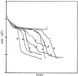
Figure 1 shows a comparison of the convergence rates of several optimization algorithms 120
when designing a triplet lens. The PSD III method is in curve A, and curve I is DLS. (The 121
and the cost is the elapsed time to get that value. Few technical fields experience an 123
improvement of this magnitude at one stroke. I am still amazed by the results. 124
This figure shows that, for the DLS method (curve I), achieving a low value of the MF (which 125
would be lower on the plot) one must go a great distance to the right, since that curve has a 126
very small slope. That translates into a great deal of time spent making countless very small 127
improvements. For years, that slow rate of convergence has been the bottleneck of the whole 128
industry. The PSD III method has broken that bottleneck. 129
130
131
Figure 1. Comparison of convergence rates for several algorithms. Curve A is for PSD III, and curve I is
132
classic DLS.
133
5. Global Optimization
134
Much effort has been expended by the industry on so-called “global optimization” methods. 135
In principle, the approach can be very simple: make a mesh of nodes, where every radius, 136
thickness, and so on takes on each of a set of values in turn, and optimize each case. Some 137
designers report evaluating a network of perhaps 200 000 nodes, and given an infinite amount 138
of time, this approach can indeed find the best of all lens constructions. But we can do 139
better. 140
The second development that contributes to the success of this new paradigm is the binary 141
search method used to find the optimum solution[12]. This concept models the lens design 142
landscape as a mountain range, with peaks and valleys all over the place. The best lens 143
solution is in the lowest valley. So how do you find it? If you are in a valley, you cannot 144
But if you are at the top of the highest mountain, you can see all the valleys in the area, and 146
that is the clue we need. The mountaintop corresponds to a lens with all plane-parallel 147
surfaces. The binary search algorithm then assigns a weak power to each element according 148
to a binary number, where 0 is a negative element and 1 is positive. By examining all values 149
of that binary number, one examines all combinations of element powers. The only 150
quantities still to be defined are what that power should be and what thicknesses and airspaces 151
to assign to the elements; those are input parameters to the algorithm. With this method, a 152
five-element lens has only 32 combinations of powers, which is far more tractable than 153
evaluating 200 000. And the results are gratifying. 154
(We note that this is actually an old idea. Brixner [13] applied this logic a generation ago, 155
running very long jobs on a mainframe computer. He was on the right track, but computer 156
technology was not up to the task, and optimization was still DLS.) 157
Let us examine the results of applying this algorithm to some classical lens constructions and 158
compare the results with what was accomplished by yesterday’s experts. 159
160
5.1 Unity-magnification Double Gauss
161
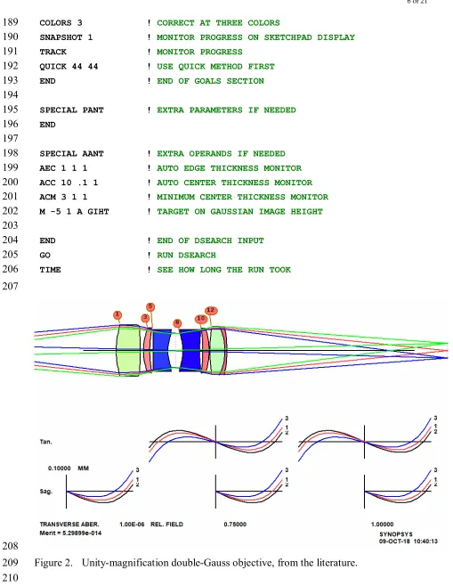
This is a classic design, the example taken from Kingslake and Johnson [1] (p. 372), shown 162
in Figure 2. Let us see what our new algorithm can do on this problem. We will use 163
DSEARCH, an option in the SYNOPSYS program. Here is the input: 164
165
CCW ! CLEAR COMMAND WINDOW
166
CORE 14 ! AUTHORIZE 14 CORES
167
TIME ! START A TIMER
168
DSEARCH 1 QUIET ! RUN DESEARCH 169
SYSTEM ! BEGIN SYSTEM SPECS
170
ID DSEARCH DG_7 ! LENS IDENTIFICATION 171
OBA 157.9075 5 17 ! FINITE OBJECT PARAMETERS 172
WAVL 0.6563 0.5876 0.4861 ! USE THESE WAVELENGTHS 173
UNITS MM ! LENS UNITS ARE MM 174
END ! END OF SYSTEM SECTION
175 176
GOALS ! DECLARE DESIGN GOALS
177
ELEMENTS 7 ! ALLOW 7 ELEMENTS 178
FNUM 4.88 1 ! TARGET F/NUMBER 179
BACK 157 .01 ! BACK FOCUS DISTANCE 180
TOTL 80 .01 ! CELL LENGTH 181
STOP MIDDLE ! PUT THE STOP IN THE MIDDLE 182
STOP FREE ! AND LET IT MOVE AROUND 183
RT 0.5 ! MEDIUM APERTURE WEIGHTING
184
FOV 0.0 0.75 1.0 0.0 0.0 ! CORRECT AT THREE FIELDS 185
FWT 5.0 3.0 1.0 1.0 1.0 ! WITH THESE WEIGHTS 186
NPASS 44 ! 44 OPTIMIZATION CYCLES WHEN DONE 187
COLORS 3 ! CORRECT AT THREE COLORS 189
SNAPSHOT 1 ! MONITOR PROGRESS ON SKETCHPAD DISPLAY 190
TRACK ! MONITOR PROGRESS
191
QUICK 44 44 ! USE QUICK METHOD FIRST 192
END ! END OF GOALS SECTION
193 194
SPECIAL PANT ! EXTRA PARAMETERS IF NEEDED 195
END 196
197
SPECIAL AANT ! EXTRA OPERANDS IF NEEDED 198
AEC 1 1 1 ! AUTO EDGE THICKNESS MONITOR 199
ACC 10 .1 1 ! AUTO CENTER THICKNESS MONITOR 200
ACM 3 1 1 ! MINIMUM CENTER THICKNESS MONITOR 201
M -5 1 A GIHT ! TARGET ON GAUSSIAN IMAGE HEIGHT 202
203
END ! END OF DSEARCH INPUT
204
GO ! RUN DSEARCH
205
TIME ! SEE HOW LONG THE RUN TOOK
206
207
208
Figure 2. Unity-magnification double-Gauss objective, from the literature. 209
210
In the above input file, we first define the system parameters, object coordinates, 211
wavelengths, and units. Then the GOALS section specifies the number of elements, first-212
order targets, fields to correct, asks for an annealing stage, and directs the program to use the 213
simple MF consisting of third and firth-order aberrations plus three real rays. This executes 215
very quickly, since little ray tracing is involved. The winners of this stage are then subjected 216
to a rigorous optimization, with grids of real rays at the requested fields (0.0, 0.75, and 1.0). 217
The SPECIAL AANT section defines additional entries we wish to go into the MF, in this 218
case controlling edge and center thicknesses and requiring the Gaussian image height to equal 219
the object height, with a sign change. That gives us the desired 1:1 imaging. 220
In these examples, we elect to correct image errors by reducing the geometric size of the spot 221
at each field point. The software can also reduce optical path difference errors (OPD), a 222
feature useful for lenses whose performance must be close to the diffraction limit, and it can 223
even control the difference in the OPD at separated points in the entrance pupil, which has 224
the effect of maximizing the diffraction MTF at a given spatial frequency. As computer 225
technology advances, the software keeps pace, adding new features as new possibilities are 226
developed. 227
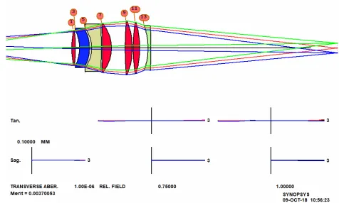
This job runs in 87.7 seconds, on our 8-core hyperthreaded PC, and the result is shown in 228
Figure 3. 229
230
Figure 3. Results from running DSEARCH on the double-Gauss problem.
231 232
The cross-hatch pattern indicates that the design at this stage uses model glasses, and the next 233
step is to replace them with real ones. We run an optimization MACro that DSEARCH has 234
created, and then run the automatic real glass option ARGLASS, specifying the Schott 235
catalog. The result, after about 30 seconds more, is in Figure 4. Clearly, this design is 236
vastly better than the classic version, even though it does not resemble the double-Gauss form 237
anymore. In less than two minutes, we have a design far better than what an expert could 238
An interesting feature of these new tools arises from the annealing stage of optimization, a 240
process that alters the design parameters by a small amount and reoptimizes, over and over. 241
Due to the chaotic nature of the lens design landscape, any small change in the initial 242
conditions sends the program to a different solution region. So if we run the same job again, 243
with the same input, we often get a rather different lens. Usually the quality is about the 244
same, and if we run it several times we get a choice of solutions. This too is an improvement 245
over classical methods, since once the old masters succeeded in getting a satisfactory design, 246
it is unlikely they would start over and try to find an even better one. But now we can easily 247
evaluate several excellent lenses and select the one we like best. Chaos in lens design is 248
discussed more fully by Dilworth [14]. 249
250
Figure 4. Final design for the double-Gauss problem, with real glass replacing the glass models.
251 252
5.2 Six-element camera lens
253
Our second example is taken from Cox, number 3-87, patent number 2892381, shown in 254
Figure 5. This is an excellent design, with about one wave of lateral color. (We have used 255
model glasses here, since the reference does not give the glass types and there are no catalog 256
258
Figure 5. Design 3-87 from Cox.
259 260
This looks like a more difficult problem. What can DSEARCH do with this one? Here is 261
the input file; 262
263
TIME 264
CORE 14 265
DSEARCH 4 QUIET 266
SYSTEM 267
ID DSEARCH 3-87 268
OBB 0 13.5 .04 269
WAVL 0.6563 0.5876 0.4861 270
271
UNITS INCH 272
END 273
GOALS 274
ELEMENTS 6 275
FNUM 8.32 276
BACK .631 .01 277
TOTL .485 .01 278
STOP MIDDLE 279
STOP FREE 280
RT 0.5 281
FOV 0.0 0.75 1.0 0.0 0.0 282
NPASS 44 284
ANNEAL 200 20 Q 285
COLORS 3 286
SNAPSHOT 10 287
TRACK 288
QUICK 44 44 289
END 290
SPECIAL PANT 291
292
END 293
SPECIAL AANT 294
295
END 296
GO 297
TIME 298
299
The result, with real glass, is shown in Figure 6. Again, it does not resemble the classic 300
form, but is far superior. There is a lesson there: the old masters often started with a well-301
known form, in this case the triplet, hoping its symmetry would yield some advantage for 302
correcting aberrations. But it is not likely they would have thought of the configuration 303
found by DSEARCH. We were able to get these results in just over one minute by pure 304
number crunching. We suspect that the original designer (Baker) invested far more time – 305
and would probably be very impressed with these new results. 306
307
Figure 6. DSEARCH results for the camera lens
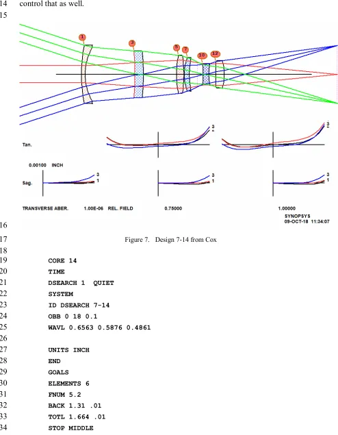
5.3 Inverse telephoto lens
310
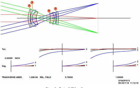
This example is also taken from Cox, number 7-14, patent 2959100. It is a pretty good 311
design, shown in Figure 7. The input for DSEARCH has an extra requirement in the 312
SPECIAL AANT section, since the lens was designed for low distortion and we want to 313
control that as well. 314
315
316
Figure 7. Design 7-14 from Cox
317 318
CORE 14 319
TIME 320
DSEARCH 1 QUIET 321
SYSTEM 322
ID DSEARCH 7-14 323
OBB 0 18 0.1 324
WAVL 0.6563 0.5876 0.4861 325
326
UNITS INCH 327
END 328
GOALS 329
ELEMENTS 6 330
FNUM 5.2 331
BACK 1.31 .01 332
TOTL 1.664 .01 333
STOP FREE 335
RT 0.5 336
FOV 0.0 0.75 1.0 0.0 0.0 337
FWT 5.0 3.0 1.0 1.0 1.0 338
NPASS 44 339
ANNEAL 200 20 Q 340
COLORS 3 341
SNAPSHOT 10 342
QUICK 44 44 343
END 344
SPECIAL PANT 345
346
END 347
SPECIAL AANT 348
ACC .25 1 .1 349
M 0 1 A P YA 1 350
S GIHT 351
END 352
GO 353
TIME 354
355
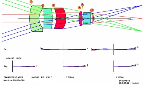
DSEARCH returns the lens in Figure 8, also better than the patented lens designed by an 356
expert. 357
358
Figure 8. DSEARCH solution to the inverse telephoto lens problem
Once again we see that numerical methods are far superior to the best that an expert designer 360
could do a generation ago. 361
But, wait. Suppose we decide those elements are too thick. The solution is simple: just 362
change the ACC monitor (Automatic Center-thickness Control) in the SPECIAL AANT 363
section so they stay below 0.1 inches, as in the patent, and run the job again. The result is 364
almost identical, except the elements are thinner. The program has options to control almost 365
anything in the lens, a vital requirement for when one is addressing a problem with numerical 366
methods. 367
368
5.4 Other methods
369
We have shown how the design search algorithm (DSEARCH) can find solutions better and 370
faster than can a human expert, even those with a lifetime of experience. But it is not the 371
only new technique that replaces theory with number crunching. 372
Let us try running the last example with a different feature [15], one that employs an idea 373
originally by Florian Bociort [16], called the saddle-point method. This method does not 374
use either a grid of designs or a binary search. Instead, it modifies an existing lens by adding 375
a thin shell at a selected surface. The shell does not change the paths of rays, but adds six 376
new degrees of freedom. The program tries every surface within a specified range and 377
optimizes each attempt. Then it selects the best of the lot and begins again, adding a new 378
element to that design, and so on until the desired number of elements is reached. 379
Here is the input for SPBUILD (saddle-point build): 380
381
SPBUILD 1 QUIET 382
SYSTEM 383
ID SPB_7-14 384
OBB 0 18 0.1 385
WAVL 0.6563 0.5876 0.4861 386 387 UNITS INCH 388 END 389 GOALS 390 ELEMENTS 6 391 FNUM 5.2 392
BACK 1.31 0.01 393
TOTL 1.664 .01 394 STOP MIDDLE 395 STOP FREE 396 RT 0.5 397
FOV 0.0 0.75 1.0 0.0 0.0 398
FWT 5.0 3.0 1.0 1.0 1.0 399
NPASS 44 400
ANNEAL 200 20 Q 401
TRACK 403
END 404
SPECIAL AANT 405
ACC .1 1 .1 406
M 0 1 A P YA 1 407
S GIHT 408
END 409
GO 410
411
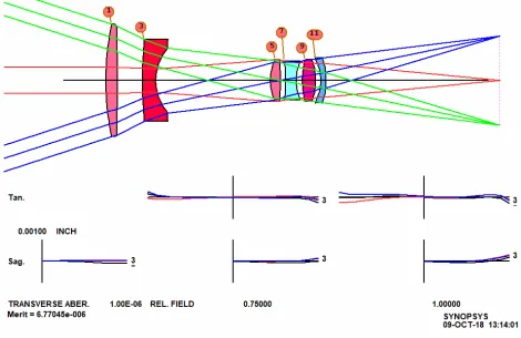
In a few minutes this input returns the lens in Figure 9, fitted with real glass as before. 412
413
Figure 9. SPBUILD solution to the inverse telephoto problem. 414
415
Here is yet another way to employ number crunching to explore the design space. Note that 416
neither this method or the binary search method of DSEARCH uses any of the classic 417
theoretical tools. The work is done via numerical methods alone, since the laws of optics 418
have been encoded in the software. 419
Although the saddle-point method can build up an entire lens from nothing, as we have seen, 420
it is most useful when one already has a design that is close to the desired goals and would 421
like to find the best place to insert an additional element. At this point, an expert would 422
likely look at how the third-order aberrations build up through the lens and using his deep 423
knowledge of theory would try to predict the optimum location. But another feature does 424
the same job much better and faster than can a human, no matter how skillful. This also uses 425
427
5.5 Zoom Lenses
428
Thus far, these examples have all been fixed-focus lenses. Can number crunching also 429
produce quality zoom lenses? 430
The question came up when a colleague sent me nine pages of hand calculations for a zoom 431
lens. He was using classical methods and knew what he was doing – but I viewed this as 432
another case where it would be nice to make the computer do all the work. The result was 433
a feature called ZSEARCH [17]. The example below shows that, although number 434
crunching does the lion’s share of the work, a skillful human designer still has an important 435
role to play. 436
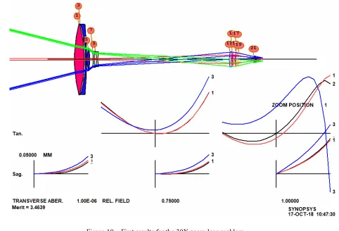
We will design a 13-element zoom lens with a 30:1 zoom ratio. Not an easy job, especially 437
since, as with the previous examples, we do not give the program any starting design. To 438
speed things up, we start with 11 elements, which means there are 2048 cases to analyze 439
utilizing the binary search method. This of course takes much longer than the previous 440
examples – but it is still much faster than doing the work by hand. This will be the input for 441
ZSEARCH: 442
443
LOG ! to keep track of things later
444
ON 98 445
TIME ! to see how long this run took 446
CORE 14 447
ZSEARCH 3 QUIET ! save results in library location 3 448
449
SYSTEM 450
ID ZSEARCH TEST 451
OBB 0 14 3 ! infinite object, 14 degrees semi field, 2.85 mm semi 452
! aperture. This defines the wide-field object 453 UNI MM 454 WAVL CDF 455 END 456 457 GOALS 458 ZOOMS 7 459
GROUPS 2 3 4 2 ! lens has four groups with 11 elements altogether 460
ZGROUP 0 Z Z 0 ! and groups 2 and 3 will zoom 461
ZFOCUS 5000 4 90 5 ! also correct range focus at 5 meters 462
FINAL ! declare the desired object at the last zoom position, 463
! which is the narrow field zoom 464
OBB 0 0.4666 90 465
466
ZSPACE NONLIN 1.7 ! other zoom objects will be nonlinearly spaced between 467
the 468
APS 19 ! put the stop on the first side of the last group 470
DELAY OFF 471
GIHT 5 5 10 ! the image height is 5 mm for all zooms, with a weight of 472
10. 473
BACK 20 .1 ! the back focus is 20 mm and will vary. A target will be 474
! added to the merit function with a low weight. 475
COLOR M ! correct all defined colors 476
ANNEAL 50 10 Q ! anneal the lens as it is optimized in both modes 477
QUICK 40 40 ! 40 passes in quick mode, 40 in real-ray mode 478
ASTART 22 479
TSTART 12 480
END 481
482
SPECIAL PANT 483
CUL 1.75 484
FUL 1.75 485
END 486
487
SPECIAL AANT 488
ACA 55 1 1 ! monitor rays to keep away from the critical angle. 489
AEC 2 1 1 490
ACM 4 1 1 491
ACC 35 1 1 492
493
LUL 600 .1 10 A TOTL 494
END 495
GO ! start ZSEARCH
496
TIME ! see how long the run took. 497
498
This runs for about 26 minutes and produces a lens that is tolerably well corrected at all seven 499
501
Figure 10. First results for the 30X zoom lens problem
502 503
When we examine the performance over 100 zooms, things are not so good, and there are 504
overlapping elements in one place, which is not surprising for so wide a range and so few 505
zooms corrected. But there are tools for these problems too. We ask the program to define 506
15 zoom positions. 507
CAM 15 SET 508
and then reoptimize and anneal. Now the lens is much better, but some elements are too 509
thin at the center or edge, and we need yet more clearance between zoom groups. We 510
modify the MF requirements to better control center and edge clearances, and also declare 511
the stop surface a real stop, so the program finds the real chief ray by iteration (instead of 512
using the default paraxial pupil calculation). 513
Here we are illustrating the new paradigm for lens design: use the search tools to find a good 514
candidate configuration, optimize it, and then modify the MF as new problems are 515
discovered; this is where the designer’s skill comes in. The process usually works, and if 516
not, then do the same with some of the other 10 configurations that were returned by the 517
search program. And running the search program once more often returns an additional 10 518
possibilities. 519
521
Figure 11. 30x zoom optimized with modified targets.
522 523
It appears that we need more than the 11 elements we started with, so now we use another 524
number-crunching tool, Automatic Element Insertion (AEI). This tool applies the saddle-525
point technique to each element to find the best place to insert a new one. 526
We add the line 527
AEI 7 1 123 0 0 0 50 10 528
to the optimization MACro and run it again. The lens is further improved, as shown in 529
Figure 12. 530
532
Figure 12. Zoom lens with element added by AEI
533 534
Although numerical methods are powerful, human insight is still important. We note that 535
the largest aberration in the MF is now the requirement to keep lens thicknesses less than one 536
inch, a target added by default by ZSEARCH. But the first element is a large lens, and to 537
correct lateral color it must be allowed to acquire whatever power it needs, and more power 538
means greater thickness. So we modify the MF, letting the thickness grow. We also add a 539
requirement that the diameter/thickness ratio should be greater than 7.0, which will increase 540
the thickness of those elements that are currently too thin, such as element number 2. Then 541
we run AEI once more, adding one more element. The result is shown in Figure 13. Figure 542
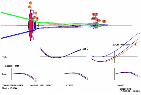
14 shows the same lens in zoom 15, the long focal length setting. This looks like an 543
excellent design. 544
Other zoom positions are even better than the extremes shown here. Now we check the 545
performance over the zoom range, using a piecewise cubic interpolation option, and find we 546
have an excellent zoom lens indeed. With these tools, we have in fact been able to go as far 547
as a 90:1 zoom lens, with three moving groups. 548
It appears that these number crunching tools work very well, and in half a day we have 549
designed a zoom lens that would have required many days or weeks of preliminary layout 550
work using older theoretical methods. 551
553
Figure 13. Zoom lens with thicknesses adjusted by the software, in zoom 1
554
555
Figure 14. Zoom lens at zoom 15
556 557
We have been surprised how, in many cases, these numerical tools have been able to correct 559
even secondary color, simply by varying the model glass parameters. An older designer 560
once insisted that doing so was impossible without using exotic materials such as calcite. 561
He was wrong, but demonstrating that fact had to wait for the development of these new tools 562
[18]. 563
It should be clear that, for these examples, numerical methods [19] vastly outperform the 564
work of expert designers from the last generation. Some of those experts embrace this new 565
technology, while others see it as a threat. I think we should all step back, evaluate the 566
technology carefully, and use its power whenever the problem can be addressed in that way. 567
The younger generation will likely have no qualms about embracing it with enthusiasm. 568
569
1. Kingslake R and Johnson R B Lens Design Fundamentals 2010 (Bellingham, WA: SPIE). 570
2. Geary J M Introduction to Lens Design 2011 (Richmond, VA: Willmann-Bell). 571
3. Dilworth D C SYNOPSYS Supplement to Joseph M Gary’s Introduction to Lens Design 2013 572
(Richmond, VA: Willmann-Bell). 573
4. Smith G H Practical Computer-Aided Lens Design 2007 (Richmond, VA: Willmann-Bell). 574
5. Laiken M Lens Design 1991 (New York: Marcel Dekker). 575
6. O’Shea D C Elements of Modern Optical Design 1985 (New York: Wiley). 576
7. Kingslake R Lens Design Fundamentals 1978 (New York: Academic). 577
8. Dilworth DC and Shafer D Man versus machine: a lens design challenge 2013 SPIE Vol. 8841. 578
9. Cox A A System of Optical Design 1964 (Waltham, MA: Focal). 579
10. Dilworth DC Improved Convergence with the pseudo-second-derivative (PSD) Optimization Method, 580
1983 SPIE Vol. 399 (159). 581
11. Dilworth DC Automatic Lens Optimization: Recent Improvements 1986 SPIE Vol. 554 (191). 582
12. Dilworth DC New Tools for the Lens Designer 2008 SPIE Vol. 7060. 583
13. https://www.researchgate.net/scientific-contributions/2039750632_BERLYN_BRIXNER. 584
14. Dilworth DC Lens Design: Automatic and Quasi-Autonomous Computational Methods and 585
Techniques 2018 (IOPscience). 586
15. Dilworth DC Novel global optimization algorithms: binary construction and the saddle-point method 587
2012 SPIE Vol. 8486. 588
16. F. Bociort and M. van Turnhout, Saddle points reveal essential properties of the merit-function 589
landscape, SPIE Newsroom (24 November 2008). 590
17. Dilworth DC A zoom lens from scratch: the case for number crunching 2016 SPIE Vol. 9947. 591
18. “Secondary color” refers to the difference in focus between a central wavelength and the longest and
592
shortest. That is historically much harder to control than primary color, which is the difference
593
between just the latter two.
594
19. SYNOPSYS, DSEARCH, ZSEARCH, ARGLASS, SPBUILD, and AEI are trademarks of Optical Systems 595
Design, Inc. 596