Self-consistent Bulge
/
Disk
/
Halo Galaxy Dynamical Modeling Using Integral Field
Kinematics
D. S. Taranu1,2 , D. Obreschkow1,2, J. J. Dubinski3, L. M. R. Fogarty2,4 , J. van de Sande4 , B. Catinella1 , L. Cortese1 , A. Moffett1, A. S. G. Robotham1 , J. T. Allen2,4 , J. Bland-Hawthorn4 , J. J. Bryant2,4,5, M. Colless2,6 , S. M. Croom2,4, F. D’Eugenio6, R. L. Davies7 , M. J. Drinkwater2,8 , S. P. Driver1 , M. Goodwin5, I. S. Konstantopoulos9, J. S. Lawrence5,
Á. R. López-Sánchez5,10 , N. P. F. Lorente5, A. M. Medling6,11,14 , J. R. Mould12 , M. S. Owers5,10, C. Power1,2 , S. N. Richards2,4,5 , and C. Tonini13
1
International Centre for Radio Astronomy Research, The University of Western Australia, 35 Stirling Highway, Crawley, WA, 6009, Australia 2
ARC Centre of Excellence for All-sky Astrophysics(CAASTRO), Australia 3
Department of Astronomy and Astrophysics, University of Toronto, 50 St. George Street, Toronto, ON, M5S 3H4, Canada 4
Sydney Institute for Astronomy, School of Physics, A28, The University of Sydney, NSW, 2006, Australia 5
Australian Astronomical Observatory, PO Box 915, North Ryde, NSW, 1670, Australia 6
Research School of Astronomy and Astrophysics, Australian National University, Canberra, ACT, 2611, Australia 7
Astrophysics, Department of Physics, University of Oxford, Denys Wilkinson Building, Keble Road, Oxford, OX1 3RH, UK 8
School of Mathematics and Physics, University of Queensland, QLD, 4072, Australia 9
Envizi Suite 213, National Innovation Centre, Australian Technology Park, 4 Cornwallis Street, Eveleigh NSW 2015, Australia 10
Department of Physics and Astronomy, Macquarie University, NSW, 2109, Australia 11
Cahill Center for Astronomy and Astrophysics California Institute of Technology, MS 249-17, Pasadena, CA, 91125, USA 12
Swinburne University, Hawthorn, VIC, 3122, Australia 13
Melbourne University, School of Physics, Parkville, VIC, 3010, Australia
Received 2017 March 10; revised 2017 August 30; accepted 2017 October 6; published 2017 November 17 Abstract
We introduce a method for modeling disk galaxies designed to take full advantage of data from integral field spectroscopy (IFS). The method fits equilibrium models to simultaneously reproduce the surface brightness, rotation, and velocity dispersion profiles of a galaxy. The models are fully self-consistent 6D distribution functions for a galaxy with a Sérsic profile stellar bulge, exponential disk, and parametric dark-matter halo, generated by an updated version of GalactICS. By creating realistic flux-weighted maps of the kinematic moments (flux, mean velocity, and dispersion), we simultaneously fit photometric and spectroscopic data using both maximum-likelihood and Bayesian (MCMC)techniques. We apply the method to a GAMA spiral galaxy (G79635)with kinematics from the SAMI Galaxy Survey and deep g- and r-band photometry from the VST-KiDS survey, comparing parameter constraints with those from traditional 2D bulge–disk decomposition. Our method returns broadly consistent results for shared parameters while constraining the mass-to-light ratios of stellar components and reproducing the HI-inferred circular velocity well beyond the limits of the SAMI data. Although the method is tailored for fitting integral field kinematic data, it can use other dynamical constraints like central fiber dispersions and HIcircular velocities, and is well-suited for modeling galaxies with a combination of deep imaging and HIand/or optical spectra(resolved or otherwise). Our implementation(MagRite)is computationally efficient and can generate well-resolved models and kinematic maps in under a minute on modern processors.
Key words:galaxies: fundamental parameters– galaxies: spiral–galaxies: structure– methods: data analysis
1. Introduction
The physical properties of nearby spiral galaxies are typically derived byfitting a number of distinct components to broadband images, either using azimuthally averaged 1D profiles or directly in 2D (e.g., Peng et al. 2002; Sánchez-Janssen et al. 2016; Johnston et al. 2017). For large surveys, common models are single Sérsic (1968) profile fits or two-component bulge–disk decompositions using an exponential disk and a de Vaucouleurs
(1959)or Sérsic profile bulge (Simard et al.2011)—appropriate parametrizations for galaxy disks and “classical” dispersion-supported bulges(Gadotti2009), respectively. Additional features like bars, spiral arms, and dust are usually only modeled for well-resolved nearby galaxies.
Photometric bulge–disk decomposition has several major drawbacks. First, the best-fit 2D model may be impossible to reproduce with more realistic 3D density profiles or a 6D phase space distribution function(DF)—a serious concern, since most
nearby galaxies are dynamically relaxed systems close to virial equilibrium. Two-dimensional models may be unable to produce a stable equilibrium system or require an unrealistic dark-matter halo density profile to reproduce the rotation curve. Therefore, it is desirable thatfitting methods exclude parameter combinations that cannot create stable equilibrium models consistent with the galaxy’s dynamics.
Bulge–disk decompositions can also produce ambiguous results. For fits with an exponential and a Sérsic profile, it is often assumed that the exponential component is a disk, whereas the Sérsic component is a bulge; however, the bulge can have a best-fit Sérsic indexns »1, leaving only the size
and ellipticity to distinguish it from the disk. Furthermore, bulges are typically centrally concentrated and compact, and therefore difficult to resolve beyond z>0.05 with seeing-limited imaging(Kelvin et al.2014).
Kinematic data can break these degeneracies, even if spatially unresolved. A single-fiber central velocity dispersion can be used to infer the presence of a “classical,” dispersion-The Astrophysical Journal,850:70(21pp), 2017 November 20 https://doi.org/10.3847/1538-4357/aa9221
© 2017. The American Astronomical Society. All rights reserved.
14
supported bulge. Similarly, an unresolved HI21 cm spectrum exhibiting a “double-horned”profile traces the orbital velocity of the neutral hydrogen gas, constraining the circular velocity at a large physical radius and(in principle)the combination of the rotation curve and HIsurface density profile.
Integral field spectroscopy (IFS) permits the inference of spatially resolved rotation and dispersion profiles by taking multiple spectra across each galaxy. Single-target surveys that are already completed include SAURON (de Zeeuw et al.2002), ATLAS3D(Cappellari et al.2011), and CALIFA
(Sánchez et al.2012,2016)—with nearly 1000 galaxies among them—whereas ongoing multiplexed surveys like SAMI
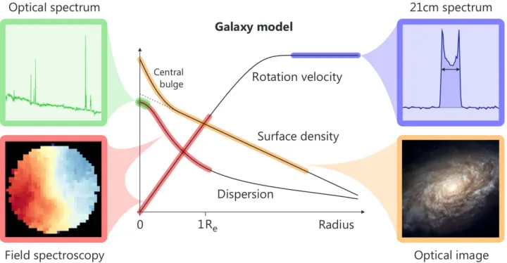
(Croom et al. 2012; Bryant et al.2015)and MaNGa (Bundy et al. 2015) have each observed ∼2000 galaxies and are expected tofinish with 3600/∼10,000, respectively. These data sets have enormous potential to constrain fundamental galaxy properties, as illustrated in Figure 1, particularly for multi-component galaxies and when combined with multiwavelength data like deep imaging and HIspectra.
There are two major challenges in interpreting IFS kinematic maps. First, extracting information on galaxy kinematics requires careful modeling to account for observational and instrumental effects, particularly “beam smearing”—the ten-dency for a point-spread function(PSF)to blur ordered rotation across a galaxy, artificially increasing the velocity dispersion. Creating spectral datacubes by stacking dithered observations has an adverse impact on image resolution, particularly in the presence of differential atmospheric refraction(Law et al.2015; Sharp et al.2015), an issue that can and should be resolved by forward modeling rather than in the data reduction process. Second, IFS maps may not have sufficient spatial coverage or signal-to-noise ratio to reach the peak of a typical galactic rotation curve, whereas even unresolved 21 cm HIspectra can, since HI disks are typically more extended than stellar disks
(e.g., Walter et al.2008; Wang et al. 2016).
Our new modeling method is designed to resolve the issues outlined above. We create dynamical models from fully self-consistent phase space DFs, then generate synthetic observa-tions of the kinematic moments to compare with observed data. Using kinematic moment maps allow for less ambiguous detections of dispersion-supported bulges. Synthetic observa-tions reproduce biases from beam smearing through the PSF/
line-spread function (LSF) and pixel discretization, allowing for simultaneousfitting of independent data sets. Finally, since the models are based on theoretically motivated analytic density profiles, they predict reasonable extrapolations beyond the limits of the observed data—vital for estimating the angular momentum in extended disks (Romanowsky & Fall 2012; Obreschkow & Glazebrook2014).
Existing galaxy dynamical modeling methods include Schwarzschild (1979)modeling (e.g., Cappellari et al.2006), Jeans’ modeling (as reviewed by Courteau et al. 2014), and made-to-measure (Syer & Tremaine 1996) and action-based modeling(e.g., Binney & McMillan2011). However, most of these methods are not specifically designed to perform bulge– disk decomposition (but see Vasiliev & Athanassoula 2015)
and many do not necessarily produce self-consistent DFs(see, e.g., Trick et al.2016, who model the Milky Way’s disk DF including a halo potential but no halo DF). Portail et al.(2017)
fit Milky Way data using a near-equilibrium M2M model with a disk, halo, bulge, and bar, but at a significant computational cost of 190 CPU-hours for 25 iterations. Our method solves both problems, generating synthetic observations of near-equilibrium bulge/disk/halo models efficiently enough to fit data from large surveys like SAMI.
In Section 2, we describe the data sources for the sample galaxy used in this pilot study. In Section3, we describe each step of the method in greater detail. In Section4, we show more detailed results and comparisons to 2D bulge–disk decomposi-tion, summarizing conclusions and outlining future directions in Section5. Three appendices detail systematic tests of model integration accuracy(AppendixA), stability(AppendixB), and fit robustness (Appendix C). Two further appendices discuss degeneracy/biases when models fit poorly (AppendixD)and when fitting inclined thick disks (Appendix E). Lastly, AppendixFdetails the GalactICS method used to build galaxy models. Future papers will provide fits to a larger sample of SAMI galaxies.
2. Data
We choose a well-resolved, massive SAMI spiral galaxy
(G79635), with M 1010.4M
» (Taylor et al. 2011) from
[image:2.612.127.487.52.239.2]broadband spectral energy distribution fits. Stellar kinematics are derived using single-Gaussian, two-moment pPXF
(Cappellari & Emsellem2004)fits to the data from the blue and red arms combined, degrading the red arm(FWHM=1.696Å, covering the redder half of the SDSSrband)to match the blue arm’s spectral resolution(2.717Å, covering the SDSSgband); see van de Sande et al. (2017) and Fogarty et al. (2015)
for details. We create “SAMIgr” flux maps by collapsing the spectral cube and masking emission and sky lines as in van de Sande et al. (2017). Flux uncertainties include approximate covariances (Sharp et al. 2015) added in quadrature to the shot/read noise, along with aflat systematic uncertainty corresponding to 10%(2.1%)of the faintest(peak) surface brightness. The dispersion maps exclude outliers from the best-fit radial profile. The PSF is a Moffat (1969) ellipse with 1 83 FWHM, derived via a ProFit(Robotham et al.2017)
fit to the reference star’sflux map(obtained from its spectral cube exactly as for the galaxy).
g- and r-band images are from the VST-KiDS survey
(de Jong et al. 2013, 2015), which covers GAMA (Driver et al. 2011) and SAMI survey regions. Uncertainties are estimated from the effective gain and local sky brightness. PSFs are Moffat ellipses with 1 16 (g)and 0 54 (r)FWHM, derived from a simultaneous ProFit fit to 39 nearby point sources. G79635 also has an HIspectrum from the ALFALFA
(Haynes et al. 2011)a.70 data release.15
3. Methods
Our method solves a nonlinear optimization problem using a parametric galaxy model, constrained by 2D kinematic moment maps or derived quantities thereof. First, a model phase space DF must be generated (Section 3.1); second, this DF must be integrated efficiently and accurately (Section 3.2); third, the integrated DF must be projected onto a datacube (position– position–velocity)and then onto kinematic maps(Section3.3). Finally, the optimization and sampling procedure is described in Section3.4. Our implementation, dubbed MagRite, is based on C/C++libraries with an R(R Core Team2016)interface forfitting.
3.1. Galaxy Models
The models are generated using an updated version, 3.0, of the GalactICS(Kuijken & Dubinski1995; Widrow et al.2008)
galaxy initial conditions code, to be detailed in a future paper
(J. J. Dubinski et al. 2017, in preparation). GalactICS has previously been used to model the surface brightness profiles and rotation curves of local group galaxies (Widrow & Dubinski 2005; Widrow et al.2008)and NGC 6503(Puglielli et al. 2010), but not 2D images/kinematic maps. The core functions of the updated code are as described in Widrow et al.
(2008). Key differences include the adoption of a logarithmic grid(previously linear), and the use of GNU Scientific Library
(Galassi2009)splines to create smooth differentiable functions for tabulated DFs and multipole expansion coefficients for the potential, both of which allow for more accurate function and derivative/integral evaluations using fewer grid elements than in earlier versions.
GalactICS generates equilibrium DFs with three components for galaxies:
1. An exponential stellar disk with massMd in, , scale radius
Rd, and scale height zd, where rµexp(-R R/ d) sech z z .2
d
( / )
2. A (deprojected) Sérsic profile stellar bulge with scale velocity vb and effective radius Rb, where
r r Rb pexp b r Rn e1 ns
r( )µ( )- (- ( ) ), p 1 0.6097 n
s
= - +
n
0.05563 s2 (Prugniel & Simien 1997), and bn scales
such thatRbis the projected half-light radius(Graham &
Driver2005).
3. A generalized Navarro et al.(1997, hereafterNFW) dark-matter halo with scale velocityvh, scale radiusrh, where
r rh 1 r rh 1
rµ[( ) (a + )(b a- )]-, anda=1,b=3 for a “pure”NFWprofile.
The minimal set of six free parameters includes a size and mass/scale velocity per component:Rbandvb(bulge);Rdand Md in, (disk); rh and vh (halo). Four parameters control the
density profiles: ns (bulge), zd (disk scale height), and α, β (halo); we fixb=3but leave the others free. Wefit the disk radial central (cylindrical) radial velocity dispersion sR0, the
square of which then declines exponentially with Rd. Finally,
we fix the streaming fractions fs b, =fs h, =0.5 (fractions of particles with a positivez-axis angular momentumLz), giving non-rotating bulges and halos.
Any component c can be truncated at a radius rt c,
with scale length drt c, , such that rtrunc( )r =rnominal( )r
r r dr
1+exp - t c, t c, -1
[ (( ) )] . Truncation is only strictly neces-sary for the halo because the NFW profile has a divergent total mass. Nonetheless, wefit the diskrt d, anddrt d, (see Section4for
the implications of this choice), but fix the bulge rt b, =10Rb (drt b, =Rb) and halort h, =50rs h, (drt h, =7.5rs h, ). This adds an
additional two free parameters to the previous nine.
GalactICS derives a DF for each spherical component using Eddington’s formula (e.g., Binney & Tremaine 2008) and iteratively computes corrections to an analytic DF describing the disk. GalactICS thenfinds a potential/density pair for each component which is consistent with these DFs. Thefinal radial density profile of each component only differs slightly from its original parametrization(see AppendixF). The key differences are that spherical components (bulge and halo) are flattened slightly in response to the presence of the disk potential and that the integrated properties of the components(e.g., disk mass Md) can deviate slightly from their input values. Although options have recently been added to GalactICS to further correct the disk density such that the output mass and profile match the input values more closely, we omitted this step pending further testing of these new features.
Despite these caveats, AppendixBshows that under normal circumstances, GalactICS models begin in near-perfect equili-brium; perturbations on the order of a few percent result only for extreme parameter combinations. More importantly, models with large Toomre (1964) Q parameters are stable against secular evolution. Although GalactICS is not restricted to generating models with large Q—this depends mostly on the values of zdand sR0—it can be guided to do so if necessary
through priors on these input parameters or on the minimumQ value at certain radii. GalactICS also converges to a near-equilibrium DF in∼30 s without expensive orbital integration
—a major advantage over Schwarzschild/made-to-measure methods and the key requirement to permit Bayesian analyses of large samples of galaxies.
15
http://egg.astro.cornell.edu/alfalfa/data/
3.2. Distribution Function Integration
The default GalactICS integration scheme samples the DF using a Monte Carlo acceptance–rejection method, which is ideal for generating unbiased, equal-mass N-body particle initial conditions. However, the rejection step is inefficient unless a suitable(i.e., strictly larger than the target distribution but only by a small margin)approximate sampling distribution is known. Unbiased sampling is not optimal for accurate integration over a uniform grid, because the fractional error is not constant but scales with density, so low-density (outer) regions have larger relative errors than the (possibly exces-sively) accurately sampled inner regions. Lastly, stochastic integration can induce spurious variations in the likelihood with small changes in parameter values. Evaluating the same model with a different random sequence or even a slightly different model with an identical random seed can result in spurious differences in integrated quantities and the resulting model likelihoods, depending on the number of samples. As a result, we chose to develop a faster and less stochastic grid-based integration scheme, which we will now describe in greater detail. For more detailed comparisons between these two integration schemes, see Appendix A.
We integrate the DF in its native cylindrical coordinate system and then project it rather than integrating over projected coordinates, as is usually done for 2D surface brightness profiles. For the remainder of this section, we will use the mathematical convention, where the azimuthal angle isθ, rather than the physics convention(f). The disk DF is parametrized as f R z v( , , R,v vq, z). It is independent ofθand symmetric over
all axes exceptvq. The DFs of the spherical components(bulge
and halo)are internally functions of energy andLz, but are
re-parametrized as f R z v( , , ) for convenience. Integrating the model over a cylindrical grid allows for some efficient
optimizations, whereas integrating down the line of sight requires repeated unique transformations at each projected position. Rotating and projecting cylindrical grid elements onto the sky plane does present a challenge. Doing so exactly requires computing the fraction of the volume of a 3D tilted ring (with a fixed height) projected within each spaxel. However, this can be roughly approximated by further discretizing each annular ring into sectors, and then assigning the mass within each sector to the spaxel containing its center of mass(in projection).
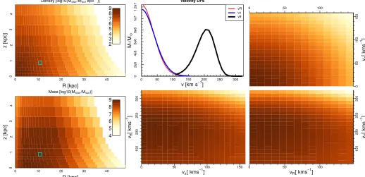
The discretized disk integration grid for G79635 is shown in Figure 2 (top-left panels). The scheme is designed to create nearly equal-mass bins. The radial grid is roughly logarithmic
—each bin covers a radius containing 1/NRof the total mass of
an ideal, thin exponential disk. The inner and outer bins are oversampled to minimize gaps at large radii and improve accuracy near the galactic center: 15% of the bins cover the inner 0.5Rd, whereas 35% cover R>3Rd. The bins
are staggered radially to spread them more evenly in projection. Vertically, the grid covers0 < <z 10zd, spaced to cover equal
masses until switching to linear spacing near the upper limit. For each R–z element, the disk DF is integrated over all
vR,v vz, q within (á ñ =vR 0)4sR, (á ñ =vz 0)4sz, and v vcirc 8s
á ñ »q q
( ) and discretized into equal-velocity bins. Figure 2 shows the integration grid for a single spatial bin, including major-axis 2D projections and 1D probability distribution functions(PDFs). Typically, the DF at most spatial coordinates in the disk is nearly (but not exactly) a Gaussian ellipsoid.
The bulge uses similar radial divisions, such that the inner and outer 20% of the bins contain 0.1Mbulge and 0.05Mbulge,
respectively, accounting for the steep slope in the Sérsic profile at small/large radii for large/small values ofns, respectively.
[image:4.612.44.562.56.307.2]The radial grid is divided into quadrants and then subdivided
into linearly spaced cells along thez-axis. The bulge DF is then integrated over allv<vesc.
3.3. Synthetic Observation Pipeline
To generate synthetic images and kinematic maps, we use an updated version of the synthetic observation pipeline described in Taranu et al.(2013)and ironically named“This Is Not A Pipeline”
(TINAP). We assume an exponentially declining star formation history for the disk,SFRµexp( (- -t t0) t), fromt0=2 Gyr
to 12.92Gyr (the universe’s age at G79635ʼsz=0.04 assuming
H0=70 km s-1Mpc-1,W =m 0.3, andW =l 0.7),fittingt-1to
avoid discontinuities at t=0. The bulge is modeled as a single burst with a free formation time tb. Both bulge and disk
components have free metallicities(ZbandZd, respectively). We
use Maraston & Strömbäck(2011)grids to computeM L in the
three bands (g, r, and SAMIgr), assuming no stellar population gradients within components. We spawn a minimum of eight
“particles” at the central R z, of each grid bin with an evenly spaced distribution from0< <q p 4, beginning at a randomθ
(the only stochastic part of the scheme)and duplicating particles in the seven remaining octants.
The two left panels of Figure3show the distributions of disk particles at twofixed radii but at different heights above/below the disk midplane, color coded by vLOS (top), along with particles at different radii but fixed heights above/below the disk midplane(bottom). After binning particles spatially and in vLOS, every spaxel produces its own vLOS PDF (right panel inset, Figure 3). These PDFs are 2D integrals of line-of-sight projections of the 3D velocity ellipsoids, and so kinematic moments are sensitive to the disk’s vertical structure and anisotropy. It is worth emphasizing that Figure2shows a very coarse integration grid with just 25 radial bins, whereas for G79635 we use 100 bins, eliminating most discreteness effects. However, the X-shaped pattern of gaps remains even for very
fine grids. This is essentially a Moiré pattern generated by overlaying an elliptical grid onto a rectangular one. The effect is minimized but not eliminated by staggering radial bins. In practice, the patterns are small enough to be virtually invisible after PSF convolution and could be avoided entirely with more sophisticated schemes for gridding the model DF, which are under development.
For stellar kinematics, vLOS cubes are convolved with the PSF and spectral line-spread function(LSF), both of which are oversampled threefold. Finally, we measure the kinematic moments in each spaxel, subtracting the LSF dispersion in quadrature for the second moment. Gaussian fits to G79635ʼs vLOS PDFs are indistinguishable from direct measurements of
vLOS,s, so we use the latter. As discussed in AppendixC, this
choice may not be suitable for galaxies with more massive and extended bulges, so we are investigating alternatives for future applications.
Generating synthetic kinematic maps requires nine addi-tional free parameters—the disk inclination and position angle, offsets for x y v, , los, and ages and metallicities for the bulge
and disk—bringing the total to 21 free parameters.
3.4. Model Fitting
Wherever possible, initial parameter estimates and prior means are obtained from 2D ProFitfits. All priors are assumed to be normal and broad (s»1 dex). We first use a robust maximum-likelihood genetic algorithm, Covariance Matrix Adaptation—Evolutionary Strategy (CMAES; Hansen 2006). We then perform Bayesian MCMC using the Componentwise Hit-And-Run Monte Carlo (CHARM) sampler of the Lapla-cesDemon R package.16The likelihood function is the sum of the log-likelihoods from each map, assuming either a
chi-Figure 3.Visualization of the model projection and map generation schemes. Left panels: scatter plots of projected disk DF samples, color coded by line-of-sight velocity(vLOS). The top-left panel shows bins at similar radii but different heights above/below the midplane, while the bottom-left panel shows a singlezbin with
ellipses at the same height above/below the midplane but at different radii. Right panel: scatter plot of DF samples for the disk and bulge, color coded byvLOS. The
inset showsvLOSDFs for the highlighted spaxel(green). Radially staggered bins are distributed more evenly in projection but still create artifacts.
16
https://cran.r-project.org/web/packages/LaplacesDemon/
[image:5.612.50.563.51.308.2]square distribution for image residuals or a sum of normally distributed residuals for kinematic maps with less well-defined errors. Residuals are defined as ci=(datai-modeli) errori
andc2= Si((datai-modeli) errori)2. Note that although we
quote reduced c2 ( red 2
c ) values, they are not used in the optimization procedure, which instead derives likelihoods from the chosen statistics’PDF directly(i.e., by calling the“dnorm” and “dchisq”functions in R).
Our CMAES code is based on the R CMAES package.17We have modified both CMAES and LaplacesDemon, implement-ing runtime limits for supercomputer queues; these versions are available on GitHub.18,19
4. Results
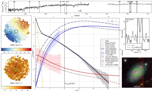
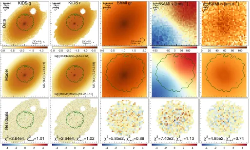
The best fit for G79635 using SAMI and KiDS g+r is shown in Figure 4. The cred2 for all of the flux maps is significantly above unity. However, the largestr-band residuals clearly trace non-axisymmetric features like spiral arms and interarm gaps, and the similarity in residuals across indepen-dent data sets is encouraging, given the systematics introduced by SAMI’s cubing procedure and single-star flux calibration. Ther-bandfit is worst simply due to its higher signal-to-noise ratio(better seeing and longer exposures thang).
Figure5shows 1D profiles azimuthally averaged over the best-fit ProFit disk ellipse, compared to a ProFit 2D double Sérsic r-band fit with a free bulge position angle. The dispersion map/ profile is overfit and the best-fit rotation curve appears to rise
slightly too steeply, as can also be seen in Figure4 (where the velocity map residuals show spatial coherence). Encouragingly, the predicted rotation curve at a fiducial radius of (3–3.4)Rd (Catinella et al. 2007) is within 10% of the independent ALFALFA HI W50=(3478 km s) -1 measurement, even
though the HIdata were not used in thefit and the SAMI data does not appear to reach the peak of the rotation curve. The lower stellar velocity could be due to asymmetric drift, as it is not unusual for stellar disks with radial dispersion support to have
10%
~ lower rotation speeds than gaseous disks (Ciardullo et al.2004; Martinsson et al.2013; Brooks et al.2017). The peak stellar velocity is also consistent with the independent
Vmaxsini=165 km s-1 circular speed derived by Cecil
et al.(2016).
The fact that the observed mean stellar velocity lies well below the circular speed curve is due to a combination of factors. First, the mean velocity withinRe,diskis decreased due
to beam smearing (compare the solid blue and dashed blue lines in Figure5). This effect is modest beyond the peak of the rotation curve(compare the solid and dashed rotation curves), although it continues to boost the observed velocity dispersion by about10 km s-1. Note that estimates of the mean velocity
and dispersion are unreliable beyond about 15 kpc, where the dispersion drops well below the 60 km s-1 velocity grid
[image:6.612.52.563.51.360.2]resolution. Also, there is some subjectivity in how 1D apertures are defined. We measure velocities and velocity dispersions using data from spaxels within 5 and 10 degrees of the major axis, respectively. The model-projected velocity without beam smearing (dashed blue curve in Figure5) is measured within the same apertures as the PSF-convolved version (solid line) and does not take into account the fact that PSF convolution
Figure 4.Best-fit G79635 model using SAMI moment 0–2 maps and KiDSg+rimages, along with residuals relative to pixel/spaxel uncertainties. KiDS images are 200×200(2ticks)while SAMI images are 36×36(1ticks).
17
https://cran.r-project.org/web/packages/cmaes/
18
https://github.com/taranu/LaplacesDemon
19
modifies isophotes as well; however, since the 1D kinematics are measured close to the major axis, this effect is minor.
In the inner few kiloparsecs, the mean velocity is suppressed both because of the presence of a non-rotating bulge and because the disk has afinite thickness, so that a large fraction of disk stars are a significant distance away from the disk midplane. Beyond this inner region, asymmetric drift and the non-zero radial and vertical velocity dispersion of the disk continue to lower the mean velocity. Observations suggest that it is not unusual for stellar disks with radial dispersion support to have ~10% lower rotation speeds than gaseous disks
(Ciardullo et al. 2004; Martinsson et al. 2013; Brooks et al.2017).
Despite alsofitting theg-band image and SAMI kinematics, the MagRite best-fit model is a better fit to the KiDSr-band image than a single-band exponential disk ProFit fit; ProFit only fits slightly better with a freensdisk.
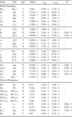
Table1lists best-fit values and uncertainties for the MagRite model parameters and several key derived quantities. Posterior distributions for selected common parameters of the MagRite and ProFitfits are shown in Figure6. Wefind that directfits to the data yield unreasonably narrow PDFs, listed as sobs. in
Table1. To test whether MagRite is the cause of this effect, we generate and fit noisy mock maps of the best-fit model (see AppendixCfor a full description of the procedure). Wefind no evidence for significant bias in the best-fit parameter values.
This form of“noise bias”can be significant in a low signal-to-noise image, as is the case in weak lensing studies (e.g., Bernstein & Jarvis2002; Refregier et al.2012). However, the parameter PDFs for fits to the mock maps are significantly broader (Table1) than when fitting the actual data—in some cases by over two orders of magnitude—and ProFit exhibits similar behavior.
As Figure4shows, an axisymmetric disk is not a goodfit to the flux maps and cannot reproduce the spiral arm structure evident in the KiDS images(especially inr). In general, models that fit data poorly underestimate uncertainties significantly, although the degree to which this occurs does depend on the model andfit statistic. This result is not immediately obvious, and we discuss it further in AppendixD. Our solution offitting mock images to obtain more realistic parameter uncertainties is necessary but likely insufficient. That is, thesmock in Table1
should be interpreted as a lower bound on the uncertainty on each parameter in the highly idealized scenario that the galaxy is perfectly described by the model. There is no obvious prescription for estimating or adjusting parameter uncertainties for models that do notfit the data well.
[image:7.612.44.564.50.361.2]Table1 also listsΔ, the difference between the ProFit and MagRite best-fit values for common parameters (whether derived orfit directly). This can be considered as an estimate of systematic uncertainties from using two different (but still similar) modeling methods. In all cases, ∣ ∣D is larger than
Figure 5.Data and 1D profiles for G79635. Clockwise from bottom left: the SAMI dispersion and velocity maps, with a 2″diameter aperture(green); the SAMI spectrum within this aperture, with emission lines excluded from thefit shaded in gray; the ALFALFA HIspectrum; RGB composite image using KiDSg-,r- and i-band images, overlaid with SAMI coverage(green). Center: azimuthally averaged, spline-fit 1D profiles(dotted lines)for thefirst three kinematic moments(KiDS r-band surface brightness—gray/black; velocity—blue; velocity dispersion—red), along with 1σuncertainties(shaded). Also shown are the best-fit MagRite(thick solid lines)and ProFit 2D double Sérsicr-bandfits(dotted lines), split among bulge(orange), disk(green), and total(purple). The background gradient in the KiDS images(most visible in the redi-band channel)was removed prior tofitting. Note that velocities are as observed and not inclination corrected, i.e.,v»vcircsin( ),i wherevcircis the circular velocity andiis the disk inclination. The best-fit MagRite modelvcircsin( )i (dotted–dashed dark blue line)lies well above the observed rotation curve, illustrating the combined effects of beam smearing, asymmetric drift, and a thick disk.
σmock—sometimes by more than an order of magnitude. This suggests that systematic uncertainties dominate over statistical uncertainties. Unfortunately, we are unaware of any robust methods for incorporating systematic uncertainties into our likelihood functions, so the only obvious solution to this issue remains increasing the model’sflexibility until it can reproduce the data.
Our testing demonstrates that MagRite will recover input parameters correctly from idealized mock data, but this does not guarantee realistic parameter values when fitting real galaxies. For example, the MagRite model has an unrealisti-cally large disk scale height, zd=1.67 kpc, and a small
truncation radius,rt d, =14.0kpc, compared to the scale length
Rd =6.52kpc. These values seem to compensate for features
in the data not otherwise described by the model. G79635ʼs disk appears steeper than exponential, and the best-fit ProFit diskns»0.8(Figure5). The small truncation radius steepens
the MagRite surface brightness profile at large radii, whereas the large scale height lowers the surface brightness along the minor axis from the galaxy center—precisely where there are two underdense interarm gaps. A model with azimuthal variations and a more general Sérsic or broken-exponential disk profile might prefer a thinner, non-truncated disk. Having said that, Muñoz-Mateos et al. (2013) fit broken-exponential profiles toSpitzer3.6μm imaging of nearly face-on disks and found a typical break radius at 2.3±0.9 inner scale lengths, so the truncation radius is not unreasonable for a Type II
(truncated, as per Freeman1970)disk.
The disk mass is also considerably higher than the total stellar mass estimated by Taylor et al. (2011) from fits to photometry alone. G79635 has a rather large estimate HImass of 1010.22M
, so it is possible that our larger disk mass is
compensating for the contribution of the gas disk to the rotation curve. This could also be the cause of the slight underprediction of the rotation curve at large radii, if it is not due to asymmetric drift. In practice, a moreflexible and betterfitting stellar mass model would likely allow the halo parameters to vary more to compensate for such inconsistencies.
The best-fit disk metallicity is quite low (log 10(Zd Z)< 0.5
- ) for such a massive disk, whereas the bulge metallicity reaches the ceiling of the Maraston & Strömbäck(2011)model grids(log 10(Zb Z)=0.3). By contrast, the disk is fairly old,
with a shortt=2.06 Gyr, while the bulge has a moderate age of 5.92Gyr. The observed galaxy colors cannot be reproduced by such a relatively simple model; in particular, the galaxy center is redder than the model, and the outskirts are significantly bluer, both by about 0.2 in g−r and with a fairly sharp transition rather than a smooth gradient. Additional model complexity (especially dust reddening and stellar population gradients) is necessary to fully reproduce galaxy colors, and full spectral modeling would be ideal. However, it is worth noting that systematic differences in the inferred stellar masses of GAMA galaxies (including the SAMI sample) can be as large as 0.2 dex depending largely on the treatment of star formation histories and dust (Wright et al. 2017), even neglecting possible variations in the initial mass function. There are also significant differences among stellar population models, stellar spectral libraries, and isochrones, which preclude making accurate estimates of stellar mass-to-light ratios even given a star formation history, and it is unclear how one might estimate the magnitude of such effects for a given galaxy.
[image:8.612.43.295.76.483.2]One potential general solution to limit parameter bias is to introduce stricter priors on model parameters based on external data. Disk scale height distributions can be constrained from independent observations of edge-on disks, and dust extinction can be estimated from Balmer line decrements. Ultimately, the best solution is to improve the model itself, which would permit the quantification of such biases. Such improvements are planned for MagRite but are not necessary to implement the method itself. For the moment, we advise caution when interpreting uncertainties from models that do not adequately reproduce known or clearly visible features in the data. This particular galaxy is well-resolved compared to average SAMI galaxies (although not uniquely so); these issues are less
Table 1
Best-fit G79635 MagRite Parameters
Name Unit loga Mean sobs. smock Δ
b
Fitted Parameters
Md in, Msimc Y 1.604 8.76e−5 1.33e−3 L Rd kpc Y 8.141e−1 2.62e−5 9.85e−4 L zd kpc Y 2.224e−1 1.83e−4 8.08e−3 L rt d, kpc Y 1.146 2.07e−4 1.67e−3 L drt d, kpc Y 7.065e−1 3.56e−4 5.26e−3 L
R0
s vsimd Y −1.281e−1 2.93e−4 2.44e−2 L vb vsim N 1.020e−2 1.80e−4 1.92e−3 L Rb kpc N −2.899e−1 1.01e−4 7.35e−3 −3.62e−2 ns N/A Y −9.970e−2 9.79e−4 2.45e−2 1.82e−1 vh vsim Y 2.693e−1 6.41e−5 1.82e−3 L rh kpc Y 8.051e−1 3.17e−4 1.47e−2 L
α N/A N 9.845e−1 1.57e−4 2.31e−2 L 1
t- Gyr−1 N 4.851e−1 1.36e−3 6.62e−3 L
tb Gyr Y 8.450e−1 1.19e−3 8.55e−3 L Zd Z Z Y −5.170e−1 1.75e−3 7.19e−3 L
Zb Z Z N 3.000e−1 8.17e−5 8.83e−3 L P.A. rad. N 8.059e−1 2.72e−4 2.08e−3 −3.26e−3
i
sin( ) rad. N 8.160e−1 1.55e−4 1.65e−3 2.09e−2 Xoff kpc N 3.732e−2 4.32e−4 5.81e−3 5.11e−2
Yoff kpc N 1.513e−2 9.68e−4 5.89e−3 5.91e−2
Vz,off km s-1 Y −1.547e−1 3.47e−1 3.55e−1 L Derived Parameters
Mde M N 10.72 1.43e−4 1.38e−3 L Mb M N 9.126 6.93e−4 1.07e−2 L
M Lg d
( ) (M Lg) N 2.726 1.47e−3 1.18e−2 L M Lr d
( ) (M Lr) Y 2.213 8.60e−4 7.42e−3 L M Lg b
( ) (M Lg) N 3.745 1.18e−2 8.79e−2 L
M Lr b
( ) (M Lr) N 2.581 7.44e−3 5.42e−2 L Ld L,r Y 10.38 1.54e−4 8.76e−4 4.46e−3 Lb L,r Y 8.715 9.91e−4 7.58e−3 2.99e−2 Re d,d kpc Y 0.9365 8.82e−5 1.10e−3 7.10e−3 Mh M Y 11.81 3.03e−4 3.33e−2 L
Notes.Fitted parameters are listed asfit internally by MagRite, whereas derived parameters are measured during or after model generation.
a
Values listed aslog 10 value unit( -1). b
MagRite value less ProFit value(where applicable), where the ProFit model has a thin Sérsic disk sharing its position angle with the bulge.
c
Msim=2.3245e9M. d
vsim=100 km s−1.
e
pronounced when fitting lower-quality data. However, as the recent public release of Subaru Hyper Suprime-Cam data
(Aihara et al. 2017) shows, high-quality, deep ground-based
imaging is rapidly becoming available for large galaxy surveys
[image:9.612.59.557.51.613.2]—even in the southern sky (Keller et al. 2007)—and so this issue cannot be ignored for much longer.
Figure 6.Triangle plot showing joint posterior parameter distributions(Lºlog 10(Lr L),Reºlog 10(Re kpc),zsºlog 10(zd kpc),nºlog 10( ), andns iis the inclination in degrees)for ProFit(blue)and MagRite(red), where the ProFit disk is a Sérsic profile and shares its position angle with the bulge. The upper-left half shows the scatter plots of accepted samples, while the bottom-right half shows the 1D and smoothed 2D probability contours. Accepted samples are colored by probability on an arbitrary scale, such that more probable points have darker and more saturated colors. Plots along the diagonals show the PDFs of accepted samples for the variable on thex-axis; to avoid crowding, they-axis ticks and labels are omitted for the three interior histograms. All posterior distributions are forfits to mock data; the best-fit parameters used to generate the mock data are plotted as circles. Note that because the ProFit thick diskfits have an unrealistically large disk scale height, the ProFit mock uses the best-fit thin diskfit parameters withzd=0.1Re d, 1.67835(equivalent to0.1Rdfor an exponential disk); this illustrates the limited constraints on disk thickness from photometry alone.
5. Conclusions
We outlined a method for kinematic bulge–disk decomposi-tion using self-consistent, DF-based dynamical models. The method can be used to model any combination of data, including deep optimal images and 1D/2D kinematic con-straints. Our GalactICS-based implementation (MagRite) is efficient enough(∼1–2 minutes per model on modern CPUs)to fit deep KiDS images and SAMI kinematic maps (Figure 5), exactly as conceptualized in Figure1.
We fit the well-resolved SAMI/GAMA galaxy G79635, showing that the best-fit parameters and posteriors are largely consistent with ProFit 2D decompositions and with the independent HIW50 constraint. This suggests that MagRite can extrapolate reasonable rotation curves even without IFS data reaching the peak of a galaxy’s rotation curve—a crucial requirement for accurate stellar mass and angular momentum estimates. In the provided appendices, we demonstrate that MagRite can fit synthetic model data with minimal biases. However, we caution that fits to real data are not immune to biases, particularly in the presence of significant non-axisym-metric features. Furthermore, we showed that poorly fitting models can seriously underestimate parameter uncertainties by yielding artificially narrow posterior PDFs. This can be mitigated, but not corrected, by estimating uncertainties from mock observations of the best-fit model.
Our example galaxy was selected as a well-resolved, fairly passive spiral galaxy with an HIdetection, but there are many more SAMI galaxies with similar quality data. The KiDS images are good enough to constrain the bulge fraction in G79635 to at most a few percent and clearly show deviations from our idealized models, which assume axisymmetric, exponential disks and simple star formation histories for each component. We therefore demonstrate that data quality is not the main impediment to improved physical modeling of galaxies, but the models themselves. G79635ʼs azimuthally averaged disk profile can be reproduced with a combination of an unusually thick and smoothly truncated exponential disk, but would be betterfit with a Sérsic or non-parametric profile disk including perturbations from spiral arms.
One shortcoming of the method using kinematic moment maps is that these must be derived independently; nonetheless, the method can be generalized tofit spectral datacubes directly
(e.g., Tabor et al. 2017), and we plan to implement this functionality within MagRite. Additional model features like spiral arms, dust attenuation/scattering (Pastrav et al. 2013), and more flexible/non-parametric density profiles are longer-term ambitions. MagRite is under active development and will be released in the near future, alongside early results from a larger SAMI sample. Parties interested in testing the code or contributing to future development are encouraged to contact the authors.
The SAMI Galaxy Survey is based on observations made at the Anglo-Australian Telescope. The Sydney-AAO Multi-object Integral field spectrograph (SAMI) was developed jointly by the University of Sydney and the Australian Astronomical Observatory. The SAMI input catalog is based on data taken from the Sloan Digital Sky Survey, the GAMA Survey, and the VST-ATLAS Survey. The SAMI Galaxy Survey is funded by the Australian Research Council Centre of Excellence for All-sky Astrophysics (CAASTRO), through project number CE110001020, and other
participating institutions. The SAMI Galaxy Survey Web site ishttp://sami-survey.org/. This work was supported by the Flagship Allocation Scheme of the NCI National Facility at the ANU. D.S.T. acknowledges support from a 2016 University of Western Australia Research Collaboration Award. B.C. acknowledges support from the Australian Research Council’s Future Fellowship(FT120100660) fund-ing scheme.
Appendix A
Integration Scheme Comparison
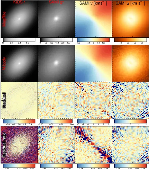
To test the accuracy and speed of the DF integration scheme described in Sections 3.2 and 3.3, we generate synthetic maps using our method and also from a high-resolution GalactICS model with 20M/0.4M disk/bulge particles, respectively. Figure7shows the maps and residuals generated using the best-fit model parameters for G79635 with both of these integration schemes. Despite the large number of particles, the MC (N-body) maps are still shot noise limited near the outskirts of the disk. Furthermore, sampling this many particles takes nearly 10 minutes on a modern test machine (Intel i5-4690 at 3.50GHz). Each accepted particle requires just over three proposals on average, meaning that nearly 70% of the computing time is effectively wasted evaluating rejected proposals. In contrast, the grid-based integration method takes under a minute and generates smoother, noise-free maps that are virtually indistinguishable from the unbiased N-body maps near the well-sampled galaxy center. This is accomplished mainly by making fewer calls to the expensive DF evaluation methods, effectively spawning dozens to hundreds of particles per DF sample.
As discussed in Section 3.3, our grid-based integration scheme is not entirely ideal. Placing evenly distributed samples at the center of each bin is computationally efficient but requires a random angular offset inθto generate smooth maps
—otherwise, the model images would have bright“spokes”at the sampled angles θ and artificial gaps between them. Similarly, binning evenly spaced ellipses onto a rectangular grid creates Moiré-like artifacts, apparent as an X-shaped residual in Figure 7. These issues could be resolved by distributing DF samples over the projected areas of elliptical rings rather than as points binned onto a rectangular grid. In principle, this would also need to be done in 3D, i.e., by generating rings corresponding to the top of one bin and the bottom of the next. These would be fairly inexpensive calculations compared to the other steps in model integration, but are somewhat complex and would be unlikely to change the PSF-convolved model maps significantly, so they are left to future revisions of MagRite.
One measurable impact of the integration scheme is the change in model likelihoods through stochasticity. To test this, we generate a series of maps for the best-fit model, varying only the random seed used to generate the angular offsets inθ. For the r-band KiDS image, the c2 value varies by about 40
from different seeds. This is an insignificant difference for a well-fitting model, but highly significant for one with a large
red 2
Appendix B Model Stability Test
To test the long-term stability of the model, we generated N-body initial conditions with GalactICS, sampling the disk/
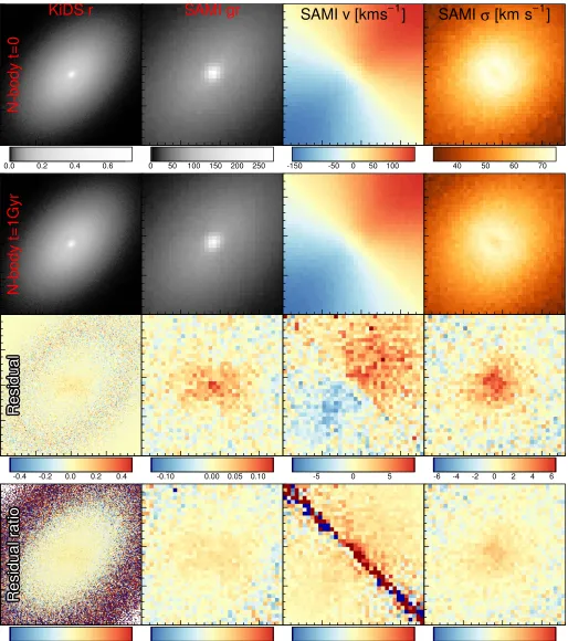
[image:11.612.48.565.52.635.2]bulge/halo with 5M/0.1M/5M particles and using softening lengths of 50/50/150 pc, respectively. We ran the model for 1Gyr with PARTREE (Dubinski 1996), using a fixed 0.196 Myr time step and an opening angle of 0.8. Figure 8
Figure 7.Comparison between maps from grid-based and Monte Carlo integration using 20M/0.4M disk/bulge particles, respectively. The residuals are shown on an absolute scale(MagRite—N-body)and as a ratio relative to the smoother MagRite map. The large relative velocity residuals along the minor axis are due to the small absolute value of the velocity; absolute differences are small.
shows the resulting maps from the evolved galaxy compared to the initial conditions. There is evidence of relaxation of the system, with the evolved model having lower central density and velocity dispersion and a shallower rotation curve.
The evolution of this model is not representative of a typical GalactICS model. As discussed in Section4, the best-fit model
has an unusually large disk scale height and small truncation radius. The initial virial ratioq = -2T W, whereTandWare the total kinetic and potential energies, respectively, is1.00275. While the deviation from unity is not large, the total energy of the system is dominated by the dark-matter halo
[image:12.612.50.564.50.630.2](with nearly 90% of the mass), so the stellar component is
likely out of equilibrium by a few percent. Accordingly, the virial ratio drops below unity by a similar factor and shows damped oscillations before reaching a new equilibrium.
We adjust the model to have a thinner disk(zd=1kpc)and
much larger truncation radius (rt d, =8rd) with the same disk
mass. This model shows virtually no evolution outside of the inner 200 pc, where there is a modest depression in the central density and velocity dispersion. We conclude that while the disk truncation parameters and scale height can in principle mimic a non-exponential(ns<1)disk, adjusting them beyond
GalactICS limits can produce unstable models and should be avoided. This could be accomplished without running simula-tions simply by placing stronger priors on model parameters or on output diagnostics like the virial ratio, but further testing is needed to determine guidelines for these limits.
Appendix C Model Fitting Test
We test the code’s ability to recover model parameters by fitting synthetic maps generated by MagRite. We assume shot noise-dominated errors for the flux maps, given a gain and mean sky brightness in counts per pixel. The higher-order SAMI moment maps require some simplifying assumptions. Kinematic constraints originate mainly from stellar absorption lines, which only cover a small fraction of typical spectra. We parametrize this effect with a simple “kinematic gain” ratio
gk,eff, which is roughly the ratio of the sum of the equivalent widths of all absorption lines to the full wavelength range. We generate a noisyflux-weightedvLOSDF for each spaxel, where
the counts in each bin are multiplied bygk,eff, andfit a Gaussian to extract the mean velocity and dispersion. Finally, we reuse the existing masks and also the velocity and dispersion error maps for consistency with the originalfits. We also adjustgk,eff
until the noise in the velocity/dispersion maps is roughly consistent with the original errors.
Figure 9 shows synthetic noisy maps for G79635 using
gk,eff =0.02. As expected, the flux maps are completely
[image:13.612.51.564.51.360.2]consistent with(nearly)normal shot noise and havecred2 »1. However, the noise in the vLOS and σ maps is not entirely identical to that from the original SAMI maps, being slightly over- and underestimated, respectively. This is not surprising, given the nonlinear nature of kinematic fits, but the mock kinematics still appear consistent with random noise without any obvious systematic bias and are usable as data for a mock fit. The possibly conservative choice of gk,eff=0.02 is motivated by the need to keep this noise consistent with the SAMI error maps; larger values lead to excessively smooth kinematic maps. When fitting, we continue to use directly measured velocity moments in the model rather than the Gaussian fits used for both the mock and real data. This is becausefitting vLOSrequires some estimate of the uncertainty of the vLOS DF in each spaxel, and it is not clear what this uncertainty should be in a noiseless model. Since G79635 has a very modest bulge, there is little difference between the two measurements; however, this may not be the case in galaxies with more massive and extended bulges, where this issue would be worth revisiting.
Figure 9.Mock G79635 maps with realistic shot noise. The kinematic maps are derived from Gaussianfits to noisyvlosDFs and therefore do not necessarily follow Poisson or(approximately)normal statistics.
Figure10shows the posterior distributions for a MagRitefit to the mock data shown in Figure9. Reassuringly, the best-fit parameters are close to the inputs, with small deviations well within the1s uncertainties. Small offsets are expected given the noise and the difference between the directly measured and fitted kinematics, but there are no significant systematic biases.
This is not to say thatfits to real data will be devoid of biases— this simply verifies that MagRite recovers unbiased parameters when the data are perfectly described by the model.
[image:14.612.63.551.50.598.2]One possible concern is that there is still some noise in the model probabilities themselves—when colored by log prob-ability, the points do not show smooth gradients in posterior
Figure 10. Triangle plot showing joint posterior distributions for model input parameters (Disk Minºlog 10(Md in, Msim), Disk Rsºlog 10(Rd kpc), r
probability from the maximum-likelihood solution. This is especially true for the fits to the observed data, which is unfortunately not clearly visible in Figure 10 because the posteriors are so narrow. This is likely due to the issues with model integration outlined in Appendix A. The main practical effect of a slightly stochastic model likelihood is that convergence to the best-fit solution can be slow, as the solution wanders between entirely artificial local maxima. This problem is exacerbated when the best-fit model is a poorfit, since even extremely small changes in input parameters can cause spurious changes in the model likelihood. Fortunately, since the actual changes in parameter values tend to be small, the impact on the posteriors from mockfits is minimal.
Since poorly fitting models tend to vastly underpredict parameter uncertainties(for reasons detailed in Appendix D
below), we suggest that uncertainties from mockfits should be considered lower bounds on the “true” parameter uncertainties. Again, this does not guarantee that there are no biases in the best-fit parameters themselves, so caution must be taken in defining priors and interpreting best-fit values in such cases. Similarly, since the mock data are idealized, they should only be interpreted as lower limits until further testing is done to quantify the impact of deviations from the assumed model parametrizations, which are necessarily present in all galaxies.
Appendix D
Parameter Uncertainties from Poorly Fitting Models It is not necessarily intuitive that poorlyfitting models can or should yield systematically smaller uncertainties than good models. Nonetheless, it is a natural consequence of the shape of some common statistical distributions. The difference in the log-likelihood (DLL) between an nσ and (n+1)σ deviation from a univariate normal distribution is -(n+0.5). The difference between 10σand 11σdeviations is then much more significant than that between 2σ and 3σ deviations, simply because the log of the PDF of a normal distribution declines as x-2 2s.
For a more practical example, the KiDS r-band image for G79635 has 25,961 usable data points (unmasked pixels). Using the chi-square distribution with 25,961 degrees of freedom as the fit statistic,20the maximum-likelihood solution for an ideal model has c2=25, 959. A 3σ deviation from a
univariate normal distribution (i.e., for a Gaussian parameter posterior) has a log-likelihood 4.5 lower than the peak. The equivalent range of likelihoods for the givenc2distribution is
25281.4, 26648.6
2
c =[ ], i.e., Dc2= -[ 677.6,-689.6] or 0.974, 1.026
red 2
c = . However, the best-fit model was only able to achieve c2=1.677 3e for the r-band image, or
6.46
red 2
c = . An increase in c2 of just 10.6 produces a
LL 4.5
D = - , so the range of acceptablec2shrinks by a factor
of approximately cred2 . Accordingly, the posterior parameter PDFs shrink by a comparable margin, depending on the linearity of the model. For a large number of degrees of freedom, this behavior approaches that of a normal distribution. Finally, we note that overfitting is strongly disfavored by the
2
c statistic—a desirable feature for data with reliable errors, as in images dominated by shot noise from a large number of
counts. For lower signal-to-noise ratio and/or where other terms like read noise are important, Poisson statistics or the so-called Cash(1979)statistic should be used.
Appendix E
Thick Disk Surface Brightness Profile Fits
As discussed in Section4, the best-fit MagRite model has an unusually large disk scale height of 1.67 kpc. We ran a number of tests by modifying ProFit to fit a thick disk with a sech2
vertical profile using a similar integration scheme as described in Section3.2. We superpose 30 Sérsic disks above and below the disk midplane by shifting the profile center along the minor axis, weighting each disk by the total mass within each vertical bin. This is not the most efficient integration method for a 3D density profile and has limited accuracy for highly inclined thick disks, but it is analogous to the MagRite method and ideal for model comparisons.
The results of fitting thick disk profiles to G79635ʼs r-band image are shown in Figure 11. First, fitting a thick exponential disk (second row/column) significantly improves the residuals over a thin exponential disk. The improvement is seen largely in the two underdense regions between the galaxy center and spiral arms(roughly NNE and SSW from the galaxy center). However, the thin Sérsic disk achieves similar improvements without significantly worsen-ing the residuals anywhere else in the disk. Thus, it is clear that a thick disk can compensate for deviations from a pure exponential disk, but not necessarily as well as by simply modifying the radial profile. Unfortunately, the best-fit ProFit disk thicknesses are unrealistically large—4.83 kpc for the exponential disk and 2.35 for the Sérsic disk.
Figure12shows the posterior distribution from the ProFit r-band fits to mock data using the same input parameters. The “Thick” model shows the same chains as in Figure 6, where the mock data were generated with a more plausible scale heightzd =0.1Re d, 1.67835(equivalent to0.1Rd for an
exponential disk), and with the other best-fit parameters taken from the best thin disk fit. A second fit was run on mock data with clipped residuals added back in. Specifically, after generating the PSF-convolved model image, we add
tanh abs 1.25 30
cs ( (c )) , whereσis the per-pixel uncertainty. The tanh scaling smoothly truncates residuals below2s, so
the disk more closely follows a Sérsic profile. Because overdensities like spiral arms and star-forming regions tend to be more significant than underdensities, the residuals have a small net positiveflux of slightly under one percent of the disk luminosity, which is reflected in a small positive bias in disk luminosity in Figure 12 compared to the input parameters. The size and Sérsic index are somewhat biased, but the scale height and axis ratio are significantly over- and underestimated, respectively, indicating that structured residuals with a small net flux can severely bias poorly constrained and/or degenerate parameters even when the model is a reasonable approximation to the data.
The fact that the scale height and inclination are highly degenerate is not surprising—if the disk’s vertical density profile is the same as its radial profile, then the scale height and inclination will be completely degenerate. Using asech2
vertical density profile rather than exponential limits does not prevent this degeneracy. MagRite achieves a tighter con-straint on the inclination by fitting the velocity map. Of course, the mass model also modifies the rotation curve, but 20
We ignore model parameters in the effective degrees of freedom, as the number of model parameters in nonlinear models is poorly defined(Andrae et al.2010).
the stellar mass is independently constrained by the flux maps. Unfortunately, the kinematic constraints on the disk scale height itself are weak. In principle, the disk dispersion is related to the disk’s vertical structure, but this is(mostly) independently parametrized in GalactICS bysR0, and SAMI’s
[image:16.612.49.565.50.562.2]spectral resolution is notfine enough to measure typical disk dispersions anyway. Thus, there are insufficient data to guarantee an accurate best-fit scale height, and a strong prior based on observations of edge-on disks should be used in practice.
Figure 11.Comparison ofr-band residuals forfive G79635 modelfits. The models include four ProFit models—thin exponential disk(“exp.thin”), thick exponential disk (“exp.thick”), thin Sérsic disk (“ser.thin”), and thick Sérsic disk (“ser.thick”)—as well as the MagRite fit. Diagonal panels show the model residuals
data model
c=( ‐ ) son a common scale(from approximately-22<c<22), where dark colors correspond to excess in the model and light colors to excess in the data. Also listed are the log-likelihoods, assuming ac2distribution; ;
red 2
Appendix F
Summary of the GalactICS Method
We provide a brief description of the methods used by GalactICS to generate DFs for composite galaxy models
[image:17.612.45.565.51.618.2]containing any number of disk-like and spherical components composed of stars, dark matter, and gas (Kuijken & Dubinski 1995; Widrow & Dubinski 2005; Widrow
Figure 12.Triangle plot showing joint posterior parameter distributions(Lºlog 10(Lr L),Reºlog 10(Re kpc),nºlog 10( ),ns zsºlog 10(zd kpc), and where qis the disk axis ratio)for the ProFitr-band Sérsic diskfits to mock data, with and without including clipped residuals from the best-fit model. Panels are structured as in Figure6. Thefit to the mock data with clipped residuals(“Thick+Resid.”)has smaller uncertainties and is also significantly biased, particularly for the scale height and inclination. The magnitude bias is due to the small net positiveflux of the residuals. For clarity, points in the upper-left quadrant are thinned by factors of 5 and 10 for the“Thick Mock”and“Thick+Resid.”samples, respectively.
et al.2008). We use the Binney & Tremaine(2008)convention below for denoting the cylindrical radius as uppercase R and spherical radius as lowercase r, as well as the physics/ISO 80000 convention of θ for the polar angle and ψ for the azimuthal angle(in contrast with Section3.2. We also use the relative binding energyºE and relative potentialY º -F, where= Y -v2 2 and vis the velocity (such thatv2 2 is
the specific kinetic energy).
A galaxy model is defined parametrically by the mass profiles for each collisionless component. Stellar bulges and dark-matter halos are defined by spherical models described by a radial profiler( )r . For example, we use the 3D deprojected Sérsic profile(Prugniel & Simien1997)to describe the bulge, which is given by
r r
R exp b r R , 1
b
e p
n e n
0 1 s
r =r
-⎛ ⎝ ⎜ ⎞⎠⎟
( ) [ ( ) ] ( )
where the parameters are the characteristic density r0, the projected half-mass radiusRe, and the the Sérsic indexns. The
two parametersbnandpare structural quantities depending on
ns. They are well-approximated by the formulae
p = -1 0.6097 ns+0.05563 ns2 ( )2
b=2ns-1 3+0.009876 ns ( )3
for 0.6<ns<10 and 10-2<R Re<103 (Terzić &
Graham2005).
There are numerous options for halo profiles depending on one’s theoretical bias, including profiles with constant density cores or power-law cusps(Merritt et al.2006). In this paper, we use a double power-law model to describe the halo,
r r
r
r
r
1 , 4
h s
s s
r =r +
a a b
- -⎛ ⎝ ⎜ ⎞ ⎠ ⎟ ⎛ ⎝ ⎜ ⎞ ⎠ ⎟ ( ) ( )
where(a b, )=(1, 3)is theNFWprofile and(a b, )=(1, 4)
is the Hernquist(1990)profile; such double power-law models are sometimes referred to as generalized NFW or Hernquist profiles.
Disks areflat axisymmetric models and are approximated by the density law
R z M
R z R R z z
,
4 exp sech 5
d d d d d d 2 2 r p = -( ) ( ) ( ) ( )
(van der Kruit & Searle1981). We emphasize that this is not the exact disk density but rather a close approximation to the final density law derived in the computation of the disk distribution function defined below.
Finally, we force the density of each component to smoothly approach zero by multiplying each profile by a truncation function. We truncate density laws using a logistic function defined by
T t( )=(1+et)-1, ( )6
with
t r r
r , 7
t
t
d
= - ( )
wherertis the truncation radius anddrtis the radial width of the
truncation interval. Equation(6)is a simple representation of a smooth step function chosen for its computational efficiency and continuous derivatives.
The method computes an axisymmetric DF for the system of the form
f(,Lz,z)=fd(,Lz,z)+fb( ) +fh( ) , ( )8
where is the relative binding energy º -E, Lz is the
z-component of the angular momentum, andz is the zenergy
defined below. The bulge and halo are functions of energy alone and so are modeled as spherical isotropic systems. The disk DF is defined as a function of three integrals of motion. Thefirst two are the usual energy andz-component of angular momentum for axisymmetric systems but we introduce a third approximate integralz= Y -z vz2 2, whereYz is the vertical
potential defined asY º Yz (R z, )- Y(R z, =0), where Ψ is
the relative gravitational potential of the systemY = -F. With these various definitions in hand, we can describe a numerical procedure for computing the component DFs. First, consider a purely spherical system composed of multiple components—we will consider modifications when including a thin disk component later. The construction of an isotropic DF
f( ) from a potential-density pair can be accomplished using Eddington’s formula(e.g., Binney & Tremaine2008),
f d d
d d d 1 8 1 . 9 2 0 2 2 0
ò
p r r = Y- Y Y + Y Y=
⎜ ⎟ ⎡ ⎣⎢ ⎛ ⎝ ⎞ ⎠ ⎤ ⎦⎥ ( ) ( )
For a system of total densityr( )r , we can compute the total potential using the integral expression
r G
r dr r r dr r r
4 1 . 10
r
r
0 2
ò
ò
p r r
Y( )= ⎡⎣⎢ ¢ ¢ ( )¢ + ¥ ¢ ¢ ( )¢ ⎤⎦⎥ ( )
To use the Eddington formula, one needs to determine the functionr( )Y and its derivatives up to second order. In general, it is difficult tofind an analytic solution so we use the following numerical method. Wefirst define a grid withnradial positions equally spaced in logarithmic space defined by
ui=logr ri 0, (11)
wherer0is a reference radius andriis the grid point radius for i=1 ..n. With this transformation, we can compute the potential at the grid positionsuias
u Gr e du e u
du e u
4 . 12 i u u u u u 0 2 3 2 i i i
ò
ò
p r rY = ¢ ¢
+ ¢ ¢ --¥ ¢ ¥ ¢ ⎡ ⎣⎢ ⎤ ⎦⎥ ( ) ( ) ( ) ( )
In practice, the infinite limits for the inner and outer integrals can be replaced with the initial and final points of the logarithmic gridu1andunwithout loss of accuracy. The inner
integral is just the mass versus radius, and this becomes insignificant if the innermost radius is sufficiently small. For the outer integral, since the density drops to zero at a finite radius defined by the truncation function, there is no need to integrate beyond this point. Accurate and stable numerical solutions are achievable with 200 grid spacings per dex, making the new method much faster.