VARIABLE MIXED STATES
FROM DISCORD TO SIGNATURES
Callum Croal
A Thesis Submitted for the Degree of PhD
at the
University of St Andrews
2016
Full metadata for this item is available in
St Andrews Research Repository
at:
http://research-repository.st-andrews.ac.uk/
Please use this identifier to cite or link to this item:
http://hdl.handle.net/10023/8969
Quantum Correlations in Continuous
Variable Mixed States
From Discord to Signatures
by
Callum Croal
Submitted for the degree of Doctor of Philosophy in Theoretical Physics
Declaration
I, Callum Croal, hereby certify that this thesis, which is approximately 41000 words in length, has been written by me, or principally by myself in collaboration with others as acknowledged, that it is the record of work carried out by me and that it has not been submitted in any previous application for a higher degree.
Date Signature of candidate
I was admitted as a candidate for the degree of PhD in September 2012; the higher study for which this is a record was carried out in the University of St Andrews between 2012 and 2016.
Date Signature of candidate
I hereby certify that the candidate has fulfilled the conditions of the Resolution and Regulations appropriate for the degree of PhD in the University of St Andrews and that the candidate is qualified to submit this thesis in application for that degree.
Copyright Agreement
In submitting this thesis to the University of St Andrews I understand that I am giving permission for it to be made available for use in accordance with the regulations of the University Library for the time being in force, subject to any copyright vested in the work not being affected thereby. I also understand that the title and the abstract will be pub-lished, and that a copy of the work may be made and supplied to any bona fide library or research worker, that my thesis will be electronically accessible for personal or research use unless exempt by award of an embargo as requested below, and that the library has the right to migrate my thesis into new electronic forms as required to ensure continued access to the thesis. I have obtained any third-party copyright permissions that may be required in order to allow such access and migration, or have requested the appropriate embargo below.
The following is an agreed request by candidate and supervisor regarding the elec-tronic publication of this thesis: Access to Printed copy and elecelec-tronic publication of thesis through the University of St Andrews.
Date Signature of candidate
Publications
The following is a list of publications that have arisen as a result of the research of this thesis.
(CCI) V. Chille, N. Quinn, C. Peuntinger, C. Croal, L. Miˇsta, C. Marquardt, G. Leuchs and N. Korolkova,
Quantum nature of Gaussian discord: experimental evidence and
role of system-environment correlations,
Phys. Rev. A91, 050301(R) (2015).
(CCII) C. Croal, C. Peuntinger, V. Chille, C. Marquardt, G. Leuchs, N. Korolkova and L. Miˇsta,
Entangling the whole by beamsplitting a part,
Phys. Rev. Lett. 115, 190501 (2015).
(CCIII) N. Quinn, C. Croal and N. Korolkova,
Quantum discord and entanglement distribution as the flow of
cor-relations through a dissipative quantum system,
Journal of Russian Laser Research36, 550 (2015).
Manuscripts in Preparation
• C. Croal, C. Peuntinger, B. Heim, I. Khan, C. Marquardt, G. Leuchs, P. Wallden, E. Andersson and N. Korolkova,
Free-space quantum signatures using heterodyne measurements,
Conference Presentations
The following is a list of conferences in which I have taken part.
1. 20th Central European Workshop on Quantum Optics (CEWQO 2013), Stockholm,
Sweden, 2013, Poster Presentation.
2. Summer School on Quantum Optics and Nanophotonics, Les Houches, France, 2013, Poster Presentation.
3. Quantum Information Scotland (QUISCO), St Andrews, Scotland, 2013, Oral Pre-sentation.
4. CLEO: QELS, San Jose, California, USA, 2014, Oral Presentation.
5. 21st Central European Workshop on Quantum Optics (CEWQO 2014), Brussels, Belgium, 2014, Oral Presentation.
6. W. E. Heraeus Seminar on Quantum Correlations Beyond Entanglement, Bad Hon-nef, Germany, 2015, Poster Presentation.
7. Workshop on Macroscopic Quantum Coherence, St Andrews, Scotland, 2015, Poster Presentation.
8. 22nd Central European Workshop on Quantum Optics (CEWQO 2015), Warsaw, Poland, 2015, Oral Presentation.
Research Visits
• Palack´y University, Olomouc, Czech Republic, January 2013.
• University of Waterloo, Ontario, Canada, May-June 2014.
Collaboration Statement
This thesis is the result of my own work carried out at the University of St Andrews between September 2012 and March 2016. Parts of the work presented in this thesis have been published in refereed scientific journals. In all cases the text in the chapters has been written entirely by me. All figures, unless explicitly stated in the text, have been produced by me.
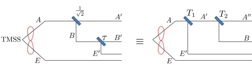
• Chapter 3 is an extension of (CCI) with some work included from (CCIII). The theoretical work for Sections 3.2 and 3.4 was carried out in collaboration with N. Quinn and L. Miˇsta. The experimental results in Section 3.2 were provided by V. Chille, C. Peuntinger, C. Marquardt and G. Leuchs. The work presented in Sections 3.3, 3.5 and 3.6 is my own with assistance provided by Norbert L¨utkenhaus and Marco Piani.
• Chapter 4 is an extension of (CCII). L. Mista developed the original idea for the project and I performed further theoretical analysis in collaboration with him. C. Peuntinger, V. Chille, C. Marquardt and G. Leuchs provided the experimental results for this chapter and aided with analysis of these results.
• Chapter 5 is a description of work performed for the manuscript in preparation enti-tled “Free-space quantum signatures using homodyne measurements”. The protocol was developed in collaboration with P. Wallden and E. Andersson. C. Peuntinger, B. Heim, I. Khan, C. Marquardt and G. Leuchs performed the experiment. I carried out analysis of the obtained data in collaboration with C. Peuntinger.
Abstract
This thesis studies continuous variable mixed states with the aim of better understanding the fundamental behaviour of quantum correlations in such states, as well as searching for applications of these correlations. I first investigate the interesting phenomenon of discord increase under local loss and explain the behaviour by considering the non-orthogonality of quantum states. I then explore the counter-intuitive result where entanglement can be created by a passive optical beamsplitter, even if the input states are classical, as long as the input states are part of a larger globally nonclassical system. This result emphasises the importance of global correlations in a quantum state, and I propose an application of this protocol in the form of quantum dense coding.
Acknowledgements
Contents
Declaration i
Copyright Agreement iii
Publications v
Conference Presentations vii
Collaboration Statement ix
Abstract xi
Acknowledgements xiii
1 Introduction 1
1.1 Introduction to Quantum Optics . . . 3
1.1.1 Quantisation of the electromagnetic field . . . 3
1.1.2 Quadrature states . . . 5
1.1.3 Coherent states . . . 6
1.1.4 Squeezed states . . . 7
1.1.5 Thermal States . . . 8
1.1.6 Purity . . . 9
1.2 Quasiprobability distributions . . . 9
1.2.1 Wigner Function . . . 9
1.2.2 Nonclassicality in Quantum Optics . . . 12
1.3 Gaussian States . . . 13
1.3.1 Definition of a Gaussian State . . . 13
1.3.2 Symplectic Analysis . . . 14
1.3.5 Standard Form . . . 18
1.4 Quantum Measurement . . . 19
1.4.1 Properties of Quantum Measurements . . . 19
1.4.2 Quantum Optical Measurements . . . 20
1.4.3 Local Quantum Measurements . . . 21
1.5 Common Experimental Techniques . . . 21
1.5.1 Stokes Operators . . . 22
1.5.2 Polarisation Squeezing . . . 23
1.5.3 Production of Correlated Mixed States . . . 24
1.5.4 Stokes Measurements . . . 25
1.6 Summary of Chapter 1 . . . 25
2 Quantum Correlations 27 2.1 Entanglement . . . 27
2.1.1 Nonlocality . . . 28
2.1.2 Separability Criteria . . . 28
2.1.3 Entanglement Measures . . . 30
2.1.4 Entanglement in Multimode States . . . 32
2.2 Quantum Discord . . . 33
2.2.1 Definition of quantum discord . . . 33
2.2.2 Properties of quantum discord . . . 35
2.2.3 Interpretations of quantum discord . . . 36
2.2.4 Gaussian quantum discord . . . 38
2.2.5 Koashi-Winter relation . . . 40
2.3 Summary of Chapter 2 . . . 41
3 Discord Increase Under Local Loss 43 3.1 Discord increase with discrete variables . . . 43
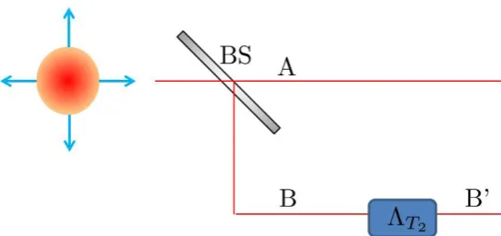
3.2 Discord increase with continuous variables . . . 45
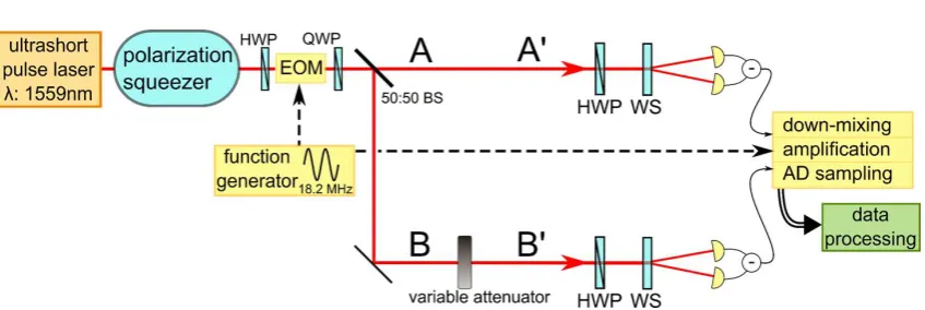
3.2.1 Discord increase scheme . . . 45
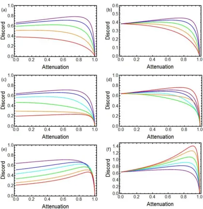
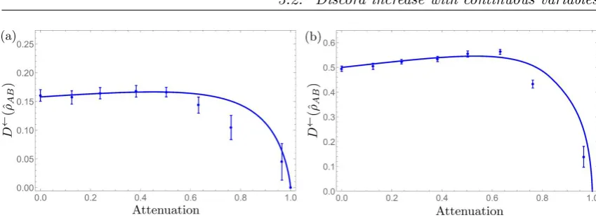
3.2.2 Experimental results . . . 49
3.4 Flow of correlations . . . 54
3.5 Alternative analysis of discord increase . . . 55
3.6 Mixture of two coherent states . . . 58
3.6.1 Calculation of Discord . . . 59
3.6.2 Behaviour of quantum discord . . . 61
3.7 Summary of Chapter 3 . . . 63
4 Entangling Power of a Beamsplitter 65 4.1 Entanglement by splitting an individually classical mode on a beamsplitter 66 4.1.1 Theoretical description . . . 66
4.1.2 Experimental implementation . . . 68
4.1.3 Conditions for the scheme to work . . . 70
4.2 Entanglement distribution by separable states . . . 73
4.2.1 Theoretical Scheme . . . 73
4.2.2 Experimental Implementation . . . 74
4.2.3 Transformation between entanglement classes . . . 75
4.3 Collaborative dense coding . . . 75
4.4 Summary of Chapter 4 . . . 80
5 Quantum Digital Signatures 81 5.1 Introduction to signatures . . . 82
5.2 Previous digital signature protocols . . . 82
5.2.1 Classical signature schemes . . . 82
5.2.2 Quantum one-way function . . . 83
5.2.3 Quantum digital signature schemes . . . 84
5.3 Quantum digital signatures with homodyne measurement . . . 88
5.3.1 Description of the protocol . . . 89
5.3.2 Security analysis . . . 91
5.3.3 Experimental implementation . . . 94
5.3.4 Theoretical models . . . 98
5.3.5 Alternative schemes based on homodyne measurement . . . 101
6.1 Future work . . . 105
6.1.1 Quantum digital signatures with unauthenticated quantum channels 105 6.1.2 Other possibilities for quantum digital signatures . . . 108
6.1.3 Nonclassical correlations and multimode entanglement . . . 109
6.1.4 Discord in quantum key distribution . . . 109
6.2 Summary . . . 110
1
Introduction
Towards the end of the 19th century, the classical theories of mechanics, thermodynamics and electromagnetism were considered to be the most important in physics. These theories all shared the common principle of determinism. That is, if one knows the initial conditions of a system one can exactly predict all future behaviour. However, this idea was completely turned on its head at the start of the 20th century with the advent of quantum theory, which introduced quantum uncertainty as an inherent property of all quantum systems. Heisenberg described this with his uncertainty principle, in which a measurement on one observable will often give a second observable unpredictable results. In particular, one can never know both the position and momentum of a quantum particle exactly.
Perhaps the strangest feature of a quantum state is the possibility of non-local be-haviour [19], which is impossible in the classical realm. This seems to contradict Einstein’s theory of special relativity, which states that no interaction can propagate faster than the speed of light. However due to the indeterministic nature of quantum mechanics, it can coexist with relativity without conflict. The first mathematical description of non-local correlations was the idea of quantum entanglement. In an entangled state of two particles, the individual particles cannot be said to have their own properties. Instead, we can only describe the global properties of the state. The result of this is that a measurement on one particle will instantaneously change the state of the other particle, no matter how far apart they are. However, whoever possesses the other particle cannot tell that the state has changed until he knows the measurement results on the first particle, which can only be learnt through the transmission of a conventional message. Therefore the transfer of information is limited by the speed of light, which is consistent with special relativity. Nevertheless, this is a counterintuitive result and the mechanism by which it occurs is still a matter of debate. However the result is undeniable and is regularly observed in laboratories throughout the world, for example in tests of Bell’s inequalities [13, 14].
behaviour [20]. In fact entanglement, non-locality and non-classicality are only equivalent for pure quantum states. In the more general case of a mixed quantum state, we require a new description of non-classicality. This has led to the introduction of quantum discord [158] as an attempt to describe all non-classical correlations in a general mixed quantum state.
Quantum information theory is the attempt to use non-classical correlations to manip-ulate information as we desire. Correlations could potentially be used to carry out secure communication and faster computation, amongst other things. Entanglement has been identified as a useful resource for quantum communication [118], however its necessity for mixed state quantum computation is unclear [54]. Recently quantum discord has also been shown to have potential uses in computation [136], and it could also have applications in quantum metrology [32]. Quantum infomation theory can be studied in either discrete variables, e.g. qubits and single photons, or continuous variables, e.g. light modes. This thesis focuses on the continuous variable case.
This thesis has two main aims. Quantum correlations between two states have been extensively studied; however, when correlations are shared between three or more states they are less well understood. I investigate quantum correlations in multimode mixed states with the aim of further understanding the fundamental behaviour of entanglement and quantum discord in these conditions. Understanding this behaviour is necessary as quantum protocols are developed that work in the real world, which inevitably involves mixed states. The second aim of this thesis is to advance the field of quantum digital signatures by developing a new signature protocol based on coherent states and homodyne detection, whereas previous protocols are based on single photon detection. Such protocols could become a widespread part of future quantum communication networks due to the importance of digital signatures.
1.1. Introduction to Quantum Optics
1.1
Introduction to Quantum Optics
In 1900, Planck asserted that light is a quantum object in his explanation of blackbody radiation [26]. Light shows wave-like properties, for example diffraction and interference. It can also be shown to have a particle nature, i.e. photons, as shown by Einstein in his description of the photoelectric effect [63]. Light also has a great ability to carry information and is used in telecommunication today. The quantum nature of light as well as its ability to contain information makes it an ideal candidate for studying quantum information theory. The basics of quantum optics, the quantum language of light, have been discussed in many excellent resources [137, 39, 77]. Here I introduce those parts that are most relevant to our investigation of continuous variable quantum information theory.
1.1.1 Quantisation of the electromagnetic field
I begin with a classical description of electromagnetism. In a dielectric medium the physi-cal quantities of light are described by the electromagnetic field strengths, the electric field
E, the displacement field D, the magnetic field Hand the magnetic induction B. These are then linked by the constitutive equations, D=0E and B=µµ0H, where 0 is the
permittivity of free space, is the permittivity of the material,µ0 is the permeability of
free space andµis the permeability of the material. In his seminal work, Maxwell linked these together to give his famous equations which can be written in differential form as
∇ ·D= 0, ∇ ·B= 0, ∇ ×E=−∂B
∂t, ∇ ×H= ∂D
∂t, (1.1)
with the additional boundary conditions that the fields vanish at infinity. Note that these Maxwell’s equations apply in regions with zero charges or currents.
Together with Newtonian mechanics, Maxwell’s equations represented a period where it was thought that everything was deterministic and it was only a matter of time before Physics would provide a complete description of the universe. With the observations of Planck and Einstein in the early 20th century, it became clear that this was no longer true, and in fact quantum uncertainty must play a role. To convert Maxwell’s equations into the quantum regime, we can make the simple assumption that the classical fields are in fact the expectation values of the quantum observables, e.g. hEˆi = E. Using this assumption it can be seen that due to their linearity, Maxwell’s equations still hold for the quantum field strengths. Thus, simply by replacing the electric field strengths with their quantum equivalents, we can use Maxwell’s equations to describe the quantum behaviour of light.
In classical electromagnetism the field strengths are often represented by the vector potential. We can do the same in the quantum case by introducing the operator of the vector potential ˆA. In doing this, we assume that the fields can be rewritten as
ˆ
E=−∂Aˆ
∂t, Bˆ =∇ ×A.ˆ (1.2)
By doing this, the middle two Maxwell’s equations immediately hold. Since the electro-magnetic field is gauge invariant we can introduce the Coulomb gauge
which ensures that the first of Maxwell’s equations also holds. Finally by rewriting the final Maxwell’s equation in terms of the vector potential, we obtain the wave equation
∇2Aˆ − 1 c2
∂2Aˆ
∂t2 = 0. (1.4)
In deriving this equation, the speed of propagation of electromagnetic waves in a vacuum emerges asc= 1/õ00.
We can now express the vector potential ˆA as a mode expansion by writing
ˆ
A(r, t) =X
k
Ak(r, t)ˆak+A∗k(r, t)ˆa
†
k
. (1.5)
In this expression, Ak(r, t) forms a complete set of classical waves that obey the Coulomb
gauge (1.3), Maxwell’s equations (1.1) and the boundary conditions. For example the plane wavesAexp(ik·r−iωt) satisfy all these conditions. All of the quantumness of light is contained in the operators ˆa†kand ˆak, which are the creation and annihilation operators
of mode k respectively, with the imposition that they are mutually adjoint.
We can now assume, as we did with Maxwell’s equations, that the quantum Hamilto-nian of the electromagnetic field can be found by taking the classical expression for the Hamiltonian and replacing the electromagnetic field strengths by their operator equiva-lents. By doing this we find the quantum Hamiltonian to be
ˆ
H= 1 2
Z
V
ˆ
E·Dˆ + ˆB·HˆdV (1.6)
with the volume integral taken over the entire space. By using the constitutive equations, writing in terms of the vector potential (1.2) and inserting the mode expansion (1.5), the Hamiltonian can be written as
ˆ
H = 1 2 ∞ X k=0 ¯ hωk ˆ
a†kˆak+ ˆakˆa†k
. (1.7)
Finally, we can use the Bose commutation relation [137]
h
ˆ
ak,ˆa†k0
i
=δk,k0 (1.8)
to write the Hamiltonian as
ˆ H= ∞ X k=0 ¯ hωk ˆ
a†kˆak+
1 2
. (1.9)
The electromagnetic field energy is thus the sum of the energies of the individual modes. The bosonic operators ˆak and ˆa†k can be thought of as the annihilation and creation
operators of photons respectively in mode k. An important result of the quantisation process is that the vacuum state |0i, that is the state with no photons, has non-zero energy. This can be seen by calculating the energy in the vacuum ash0|Hˆ|0i=P∞
k=0 ¯ hωk
2 ,
1.1. Introduction to Quantum Optics
result is that the electromagnetic field possesses energy even when there are no photons present. This is known as the zero-point energy and results in experimentally confirmed phenomena, for example the Casimir force [36], which causes two parallel conductors separated by the vacuum to feel an attractive force.
Now that the electromagnetic field is quantised and creation/annihilation operators have been introduced we can move onto alternative representations of continuous variable quantum states. In what follows, ¯h= 1 unless otherwise stated.
1.1.2 Quadrature states
In the following discussion I restrict to single mode representations where the subscript k
has been dropped for convenience. I start by introducing the quadrature operators ˆxand ˆ
p, which can be written in terms of the creation and annihilation operators as
ˆ
x= √1
2
ˆ
a†+ ˆa, pˆ= √i
2
ˆ
a†−aˆ. (1.10)
These quadratures are often considered to be the in-phase and out-of-phase components of the electric field amplitude with respect to a reference phase. The operators are canonically conjugate and satisfy the commutation relation
[ˆx,pˆ] =i. (1.11)
Although these operators have no relation to the position and momentum of a photon, this commutation relation allows us to treat ˆx and ˆp as perfect examples of position and momentum-like properties. In fact, by expressing the photon number operator ˆn= ˆa†aˆin terms of the quadrature operators, we obtain the equation
ˆ
H≡ˆn+1 2 = ˆ x2 2 + ˆ p2
2 . (1.12)
This equation represents the energy of a quantum harmonic oscillator of unity mass and frequency; the single mode is thus the electromagnetic oscillator with position ˆx and momentum ˆp!
We can now introduce the quadrature states |xi and |pi as the eigenstates of the quadrature operators. That is
ˆ
x|xi=x|xi, pˆ|pi=p|pi. (1.13)
These states are both orthogonal and complete:
hx|x0i=δ(x−x0), hp|p0i=δ(p−p0),
Z ∞
−∞
|xihx|dx=
Z ∞
−∞
|pihp|dp= 1 (1.14)
and are linked together by the Fourier transformation
|xi= √1
2π
Z ∞
−∞
exp(−ixp)|pidp, |pi= √1
2π
Z ∞
−∞
exp(+ixp)|xidx. (1.15)
can be used to define the quadrature wave functions
ψ(x) =hx|ψi, ψe(p) =hp|ψi. (1.16)
Unlike the quadrature states, these are physical with their moduli squared giving the probability distributions of the pure state |ψi for each of the quadratures.
1.1.3 Coherent states
Ideal laser light is a coherent electromagnetic wave that is the closest possible analogue to a classical electromagnetic wave. Since it has a well-defined amplitude the coherent states are defined as those that are eigenstates of the annihilation, or amplitude, operator ˆa,
ˆ
a|αi=α|αi. (1.17)
Coherent states were first suggested by Schr¨odinger [179] as a response to a claim by Lorentz that quantum mechanics was not consistent with classical behaviour of light. They were then considered in mathematical detail by Roy J. Glauber [90, 88], which is why coherent states are sometimes known as Glauber states.
It can be seen that the photon number distribution for a coherent state is given by the Poissonian distribution as
pn=
|α|2n
n! e −|α|2
. (1.18)
This is exactly the same probability distribution that we would get from a set of randomly distributed classical particles. Therefore a Poissonian distribution is essentially classical which allows us to say that coherent states give us the most classical quantum description of light.
It is important to note that the quantum vacuum is itself a coherent state, as it satisfies Eqn. (1.17) forα= 0. To more clearly examine the link between the vacuum and coherent states, consider the displacement operator
ˆ
D(α) = exp(αˆa†−α∗ˆa). (1.19)
Using this operator, a coherent state can be written, and therefore thought of, as a dis-placed vacuum state
|αi= ˆD(α)|0i. (1.20) To study this link in more detail, we can break up the amplitude α into its real and imaginary parts
α= √1
2(x0+ip0), (1.21)
and therefore express the displacement operator in terms of the quadratures ˆ
D= exp(ip0xˆ−ix0pˆ). (1.22)
The values of x0 and p0 are the displacements of the vacuum in the amplitude and phase
1.1. Introduction to Quantum Optics
vacuum states, we obtain the position wave function of a coherent state
ψα(x) =π−1/4exp
−(x−x0)
2
2 +ip0x−
ip0x0
2
. (1.23)
Similarly, the momentum wave function is
˜
ψα(p) =π−1/4exp
−(p−p0)
2
2 −ix0p+
ip0x0
2
. (1.24)
These wavefunctions show us that the quadrature probability distributions |ψα(x)|2 and
|ψ˜α(p)|2 are Gaussian with the same width as the vacuum; they are simply shifted by
the real values x0 and p0. This means that only vacuum noise, which is impossible to
eliminate, disturbs the quadrature amplitudes of a coherent state. Therefore coherent states possess the minimum possible uncertainty allowed by quantum mechanics. This is part of the reason that coherent states are such a valuable experimental tool.
1.1.4 Squeezed states
One of the basic assertions of quantum mechanics is that all quantum systems inherently contain uncertainty. In quantum optics this is demonstrated by Heisenberg’s uncertainty principle [104]
∆x∆p≥ 1
2. (1.25)
In a vacuum or coherent state we know that the position and momentum quadratures have the same uncertainty and Heisenberg’s uncertainty principle is saturated. This means the uncertainties in thex and p-quadratures are given by ∆x= ∆p= 1/√2.
States that saturate Eqn. (1.25) are called minimum uncertainty states for obvious reasons. Previously, we saw that coherent states are such states with equal uncertainty in the position and momentum quadratures; however these are not the only type of minimum uncertainty state. In a brilliantly simple proof [163] (translation [164]), Pauli demonstrated that a minimum uncertainty state |φi that saturates Eqn. (1.25) must also satisfy the equation
1 2
x
∆2xφ(x) +
∂
∂xφ(x) = 0 (1.26)
where ∆2xis the variance of the position quadrature. Eqn.(1.26) allows us to have states where the variance in one quadrature reduces below 1/2 as long as the variance in the conjugate quadrature increases accordingly. States of this form are known as squeezed states and are important in many quantum protocols.
To parametrise the squeezing I introduce the real parameterr so the variances can be written as
∆2x= 1 2e
−2r, ∆2p= 1
2e
2r. (1.27)
Just as coherent states can be expressed as displaced vacuum states, so squeezed states can be expressed as squeezed vacuum states by introducing the squeezing operator
ˆ
S(r) = exp
hr
2
ˆ
a2−ˆa†2
i
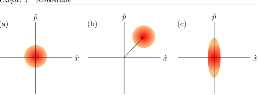
Figure 1.1: On a plot of position x and momentum p, a classical system could be represented as a point with an exact position and momentum. In a quantum system there is always inherent uncertainty in each of the quadratures. In the phase-space representation, the width of the ellipse in each quadrature gives the variance in that quadrature. (a) A vacuum state has equal uncertainty in each quadrature so is represented by a circle. It is also a minimum uncertainty state so the variance in each quadrature is 1/2. The vacuum state is centred on the origin. (b) A coherent state has the same uncertainty as the vacuum so can again be represented as a circle, however the coherent state is not centred on the origin. In this way we see why we can say that the coherent state is a displaced vacuum. (c) A squeezed state has reduced uncertainty in one quadrature and increased uncertainty in the other. Therefore we represent a squeezed state by an ellipse. In this case the vacuum has been squeezed in the ˆx-quadrature and anti-squeezed in the ˆp-quadrature.
Applying this operator to the vacuum results in the squeezed vacuum state
|φi= ˆS(r)|0i. (1.29)
Applying the displacement operator to a squeezed state changes the average value of the quadratures without altering their variance. In fact, all minimum uncertainty states are displaced squeezed vacua, as long as the squeezing can take place in any direction. Due to the nonlinearity in Eqn. (1.28), squeezing is not a passive operation; it alters the number of photons in a state, which means that even a squeezed vacuum carries more energy than the vacuum itself.
Finally, it is important to note that, unlike coherent states, squeezed states are com-pletely non-classical. The reduction of the noise in one of the quadratures is one illustration of its quantum properties. Another, is that if a squeezed vacuum is split on a beamsplitter, entanglement between the two outgoing modes is established [128, 29]. Entanglement is the strongest indicator of a quantum system, and the fact that it can be simply produced using a squeezed state, whereas it is impossible to create using passive operations on coher-ent states, is an obvious demonstration of the quantumness of squeezed states. Note that the quantumness of squeezed states can also be seen without the need for entanglement. This quantumness can be used, for example to implement measurements with accuracy beyond the classical limit. This nonclassicality can be observed from the photon statistics of squeezed states, for example in the second order correlation function [147].
A depiction of a vacuum state, coherent state and squeezed state in phase-space is seen in Fig. 1.1.
1.1.5 Thermal States
1.2. Quasiprobability distributions
thermal state is in a state of maximal disorder so it has high entropy and is a mixed state. In the context of this work, this means that a thermal state is one that maximises the von Neumann entropy
S ≡ −Tr( ˆρlog ˆρ) (1.30)
for fixed energy Tr( ˆρˆa†ˆa) = ¯n, where ¯n≥0 is the mean number of photons. The thermal state that satisfies this condition is one that has equal variance in both quadratures, where the variance depends on the mean photon number. Combining thermal states with the displacement and squeezing operators produces a class of states important for this thesis, namely the set of Gaussian states.
1.1.6 Purity
An important concept in quantum information theory is the purity of a quantum state. If a quantum state is pure it can be represented by a wavefunction |φi, however if it is mixed it must be represented by a density operator ˆρ. The purity of a quantum state ˆρ is defined as
P ≡tr( ˆρ2), (1.31)
whereP satisfies the relation 0< P ≤1, with P = 1 corresponding to a pure state. The von-Neumann entropy S( ˆρ) in Eq. (1.30) can also be used to differentiate between pure and mixed states, with the condition thatS( ˆρ) = 0 for pure states andS( ˆρ)>0 for mixed states. Since the von-Neumann entropy can be interpreted as the disorder in a system, this means that pure states have zero disorder, in other words we have perfect knowledge of pure states. Mixed states, on the other hand, always involve some classical ignorance; they are essentially an admission that we have lost information about a state. This information is lost via interactions with the unmeasured “environment” and is difficult to recover in most situations. All mixed states can be thought of as part of a larger pure state that holds all the information that has been lost to the environment. Of course in any real experiment, studied systems are constantly interacting with the environment and are therefore almost always in a mixed state. Therefore understanding the properties of mixed states, and how best to make use of them, is of vital importance in quantum information theory.
1.2
Quasiprobability distributions
1.2.1 Wigner Function
Classically we consider the phase space distribution as a joint probability distribution, however in the quantum case we can no longer do this. The most obvious reason is that in the quantum case it is impossible to know bothx and pat the same time, which can lead to a negative phase space distribution. Instead, this quantum phase space distribution is called a quasiprobability distribution and certain conditions are imposed on it so that it is useful for calculating observables [25]. This work follows the method of Leonhardt [137] to derive a useful form for the quasiprobability distribution describing a quantum state. In a classical probability distribution the marginal distributions give the probability distributions for the individual quadratures, i.e.
Z ∞
−∞
W(x, p)dx= pr(p),
Z ∞
−∞
W(x, p)dp= pr(x) (1.32)
where pr signifies a probability distribution. This is also required to hold for a quantum quasiprobability distribution. For a function to be considered a quasiprobability distribu-tion it must also be normalised
Z ∞
−∞
W(x, p)dxdp= 1 (1.33)
and real as a representation of Hermitian operators. Finally, if the density matrix ˆρ de-scribing the quantum state is rotated by an angleθ, then the quasiprobability distribution should transform as
W(x, p)→W(xcosθ−psinθ, xsinθ+pcosθ). (1.34)
This relation means that the position probability distribution pr(x, θ) can be calculated for all anglesθ using the equation
pr(x, θ)≡ hx|Uˆ(θ) ˆρUˆ†(θ)|xi=
Z ∞
−∞
W(xcosθ−psinθ, xsinθ+pcosθ)dp. (1.35)
The first part of this equation follows from the definition of a probability density, and the second part is a generalisation of equation (1.32) for any projection angle. This equation ensures that the equations in (1.32) are satisfied; θ = π/2 reduces to the first equation and θ= 0 reduces to the second. Equation (1.35) also tiesW(x, p) to quantum mechanics for the first time by introducing a connection to the density matrix. To fully understand the importance of this relationship, the Fourier transformed quasiprobability distribution
˜
W(u, v), called the characteristic function, has to be introduced:
˜
W(u, v)≡
Z ∞
−∞
Z ∞
−∞
W(x, p) exp(−iux−ivp)dxdp, (1.36)
as does the Fourier transformed position probability distribution
˜
pr(ξ, θ)≡
Z ∞
−∞
pr(x, θ) exp(−iξx)dx. (1.37)
Inserting the second part of equation (1.35) into (1.37) results in the equation
˜
pr(ξ, θ) =
Z ∞
−∞
Z ∞
−∞
1.2. Quasiprobability distributions
wherex0 and p0 are the rotated quadratures
x0 =xcosθ−psinθ, p0=xsinθ+pcosθ. (1.39)
Since x=x0cosθ+p0sinθfrom (1.39), the right hand side of (1.38) is just the definition of the characteristic function in a transformed coordinate system, i.e.
˜
pr(ξ, θ) = ˜W(ξcosθ, ξsinθ). (1.40)
This means that the Fourier transformed position probability distribution is simply the characteristic function in polar coordinates.
We can now go back and use the first part of Eq. (1.35) to make use of the quantum nature of the quasiprobability distribution. Inserting it into Eq. (1.37) results in
˜
pr(ξ, θ) =
Z ∞
−∞
hx|Uˆ(θ) ˆρUˆ†(θ)|xiexp(−iξxˆ)dx
= trnρˆUˆ†(θ) exp(−iξxˆ) ˆU(θ)o.
(1.41)
Now, since the second line of this equation causes a rotation of the quadrature operators, and the Fourier transformed probability distribution is the characteristic function in polar coordinates, we get the result
˜
W(u, v) = tr{ρˆexp(−iuxˆ−ivpˆ}. (1.42)
This means that the characteristic function is the quantum Fourier transform of the density operator. Since the characteristic function is defined as the Fourier transform ofW(x, p), the quasiprobability functionW(x, p) must be very closely related to the density operator ˆ
ρ. In fact, they are both one-to-one representations of the quantum state and so can be used interchangably to calculate properties of the quantum state.
There are many possible quasiprobability functions that are consistent with most of the above, but the only function for which the marginal distributions give the true statistics of the quadratures is the Wigner function. The Wigner function was first proposed by Eugene Wigner in 1969 [220], and can be written in terms of x and p as
W(x, p) = 1 2π
Z ∞
−∞
exp(ipx)Dx−q
2 ρˆ x+ q 2 E dq. (1.43)
This was “chosen from all possible expressions, because it seems to be the simplest” [220]. The Wigner function is a quasiprobability distribution that forms a classical-like phase space distribution for quantum mechanics. It is derived from Eq. (1.42) by application of the Baker-Campbell-Hausdorff formula
exp(−iuxˆ−ivpˆ) = expuv 2
exp(−iuxˆ) exp(−ivpˆ). (1.44)
The most important property of the Wigner function is the overlap formula, which when written for two Hermitian operators ˆρ and ˆO, takes the form
TrhρˆOˆi= 2π
Z ∞
−∞
This means that one can calculate the expectation value of any operator ˆO in a quantum state ˆρusing only the Wigner function. Thus the Wigner function can be used to calculate expectation values of physical observables, which is the intended purpose for our quantum phase space distribution. An important property of the Wigner function is that it is not necessarily positive. This is one of the reasons why it can only be called a quasiprobability distribution. In fact this property of the Wigner function has a useful physical interpreta-tion. Negativity of the Wigner function for a quantum state is often used as a signature of nonclassicality [144], although not all nonclassical states have a negative Wigner function.
1.2.2 Nonclassicality in Quantum Optics
As stated previously, there are many possible quasiprobability distributions that can be chosen to represent a quantum state. The Wigner function is the most commonly used, partially because it has a simple description, but also because it is a good compromise between a classical phase space distribution and a quantum mechanical representation. However, there are a number of other possibilities, some of which are particularly useful.
One of these representations is called theQ function, defined as
Q(x, p)≡ 1 π
Z ∞
−∞
Z ∞
−∞
W(x0, p0) exp −(x−x0)2−(p−p0)2
dx0dp0. (1.46)
From the overlap formula (1.45) it can be seen that the Q function defines the overlap between the Wigner function of the state ˆρ and that of a coherent state, i.e. it gives the probability distribution for finding the coherent states|αiin the state ˆρ, because
Q(x, p) = 1
2πtr{ρˆ|αihα|}=
1
2πhα|ρˆ|αi. (1.47)
From this, it can be seen that the Q function must always be positive. This means that all the negativities that could be present in the Wigner function no longer exist in the
Q function. For this reason the Q function is sometimes called the smoothed Wigner function. Since this smoothing eliminates all the negativities, they must be localised to small areas of the Wigner function. The Qfunction also has an application in calculating anti-normally ordered expectation values of the form tr{ρˆˆaˆa†}.
Normally ordered expectation values play an important role in some areas of quantum optics [147] and a quasiprobability distribution for normal ordering is desirable. Similarly to the way that smoothing the Wigner function gives the quasiprobability for anti-normally ordered states, the Wigner function is obtained by smoothing the quasiprobability function for normal ordering, i.e.,
W(x, p) =
Z ∞
−∞
Z ∞
−∞
P(x0, p0)
1
πexp −(x−x0)
2−(p−p 0)2
dx0dp0, (1.48)
where P(x0, p0) is theP function, the quasiprobability distribution for normal ordering.
TheP function is also often known as the Glauber-Sudarshan due to its close relation-ship to coherent states [89, 199]. This was famously expressed in the optical equivalence theorem [129] ˆ ρ= Z ∞ −∞ Z ∞ −∞
1.3. Gaussian States
This equation shows that theP function is the decomposition of the density operator into coherent states. This means that if the P function is positive everywhere, then the state can be written as a statistical mixture of coherent states. In Eq. (1.48) we saw that the Wigner function is the smoothedP function; this means that theP function is even more ill-behaved than the Wigner function, which itself can already be negative. Therefore the
P function can have some very strange behaviour, including derivatives of the Dirac delta function. In fact, the behaviour of the P function has a very important role in quantum optics. States that have a completely positive P function are considered classical, and all others are thus nonclassical. This emphasises the consideration of coherent states as the classical states, since only those that can be expressed as a statistical mixture of coherent states are considered classical. Note that theP function, theQfunction and the Wigner function are all one-to-one correspondences to the quantum state ˆρ, and therefore knowledge of any one of these functions is enough to completely describe the quantum state.
It is important to note here that there are two different notions of nonclassicality used in this thesis and in the study of quantum optics. There is the definition stated above based on the behaviour of theP function. This relates to the nonclassicality of an individual quantum state, with squeezed states in particular being considered nonclassical. In addition, there is a definition that deals with the nonclassicality of correlations and is closely related to quantum discord, which is introduced in detail in Chapter 2. In this thesis, the term “nonclassical” is used to refer to both types of nonclassicality, and it should be inferred from context which definition is intended. Ferraro and Paris [73] provide a detailed discussion on the relationship between the two definitions.
1.3
Gaussian States
1.3.1 Definition of a Gaussian State
Up to this point, I have focussed on describing quantum states that consist of a single optical mode, for example squeezed states and coherent states. Since most interesting phenomena involve states of more than one mode, it is clearly necessary to be able to describe states with multiple modes, in principle up to an arbitrary number N, although two- and three-mode states are most important for this thesis. To aid discussion the vector of quadratures
ˆ
x≡(ˆx1,pˆ1, ...,xˆN,pˆN)T, (1.50)
is introduced, where the quadratures are defined in terms of the bosonic field operators in Eq. (1.10). The construction of this vector allows the commutation relations between all the quadratures to be written in a concise way
[ˆxi,xˆj] =iΩij, (1.51)
where the matrix Ωof the form
Ω≡ N
M
k=1
ω, ω≡
0 1
−1 0
, (1.52)
has been introduced, which is known as the symplectic form.
moments. The first moment is the mean value of the quadratures
¯
x≡ hxˆi= tr(ˆxρˆ), (1.53)
and the second moment is the covariance matrixV defined as
Vij ≡ h∆ˆxi∆ˆxj+ ∆ˆxj∆ˆxii, (1.54)
where ∆ˆxi = ˆxi−hxˆii. The diagonal elements of the covariance matrix are the variances of
the individual quadratures, and the off-diagonal terms describe the correlations between different quadratures, both within a single mode and between different modes.
The first two statistical moments have a particular importance for the class of Gaussian states. Gaussian states are those that have a Gaussian Wigner function, i.e. one of the form
W(x) = exp[−1/2(x−x¯)
TV−1(x−x¯)]
(2π)N√detV . (1.55)
A Gaussian state is always fully described by its first two statistical moments, which is why the Wigner function depends only on these. This is in contrast to non-Gaussian states, where all the statistical moments must be known to fully characterise the state, which is not very useful considering there are infinitely many of them! This property clearly demonstrates the appeal of Gaussian states. States that are close to being Gaussian states are well approximated by their first two statistical moments. How close a state is to a Gaussian state can be determined by studying the higher order statistical moments. The appeal of Gaussian states is further enhanced by the fact that most quantum optical states in practical use are Gaussian, or at least close approximations. In fact it is difficult to create states that have significant non-Gaussianity and there is a strong area of research that aims to produce them. Photon number states and “Schr¨odinger cat” states are two popular examples of non-Gaussian states that have practical uses and are therefore of interest. For a rigorous review of quantum information theory with Gaussian states, see, for example, [216].
1.3.2 Symplectic Analysis
In most cases, the mean value of quadratures doesn’t affect the properties of a quantum state, therefore for Gaussian states the most important quantity is the covariance ma-trix. One crucial example of the importance of the covariance matrix is in a version of Heisenburg’s uncertainty principle [194]
V+iΩ≥0, (1.56)
which follows from the commutation relations in Eq. (1.51). As can be seen above, the symplectic form comes into the uncertainty relation along with the covariance matrix. In fact the symplectic group, of which the symplectic form is a part, provides the framework for investigating Gaussian states, and it gives its name to the branch of mathematics used to study them, symplectic analysis.
gen-1.3. Gaussian States
erated from Hamiltonians ˆH by U = exp(−iH/ˆ 2) where ˆH are second order polynomials of the field operators. In terms of the quadrature operators, the unitary operationsU can be fully described by the mapping
(S,d) : ˆx→Sxˆ+d, (1.57)
where d is a vector of real numbers and S is a 2N ×2N real matrix. Crucially, any operation must preserve the commutation relations, which happens in this case when the matrixS preserves the symplectic form, i.e.,
SΩST =Ω. (1.58)
Transformations of this form are called symplectic transformations and this further empha-sises the importance of the symplectic form in the study of Gaussian states. Upon action of a Gaussian unitary operation, the statistical moments of a quantum state transform as
¯
x→S¯x+d, V→SVST. (1.59)
Since we are mostly interested in the covariance matrix, it can be seen that the matrixS
is the most important characteristic of a Gaussian transformation.
Probably the most important result in symplectic analysis is Williamson’s theorem [222]. It shows that any covariance matrix V can be put into a diagonal form using a symplectic matrix S such that
V=SV⊕ST, V⊕=
N
M
k=1
νk1, (1.60)
where the diagonal matrix V⊕ is the Williamson form of Vand 1 is the two-dimensional identity matrix. TheN positive real numbers νk are the symplectic eigenvalues ofV and
can be calculated as the magnitude of the eigenvalues of the matrixiΩV. The symplectic eigenvalues are important as they can be used to calculate a number of fundamental properties of a system. For example, the uncertainty relation is equivalent to the statement
νk≥1, i.e. the symplectic eigenvalues of a physical quantum state must be greater than or
equal to one. The symplectic eigenvalues can also be used to calculate the von-Neumann entropy of a Gaussian state [108], using the equation
S( ˆρ) =
N
X
k=1
g(νk), g(x)≡
x+ 1 2
log
x+ 1 2
−
x−1 2
log
x−1 2
. (1.61)
From this equation and remembering that the von-Neumann entropy is zero for a pure state, it can be seen that the symplectic eigenvalues of a pure state are all equal to one, whereas for a mixed state at least one of them is greater than one. The purity, P, of a Gaussian state can also be more easily calculated directly from the covariance matrix V
by the equationP = 1/√detV, which means that detV = 1 for pure states and detV>1 for mixed states.
(1.60), a purification of this state has the covariance matrix
Vp =
V SC CTST V⊕
, C≡
N
M
k−1
q
ν2
k−1σz, (1.62)
where σz = diag(1,−1) is the Pauli-z matrix. For a general mixed state, there are many
possible purifications of which this is only one of them. A purification that is of particular interest is the one of smallest dimension; unfortunately this method doesn’t always give that purification, and it is often difficult to determine the purification with the fewest number of modes. Caruso et al. [35] developed a method to calculate the minimum number of modes required for a purification.
1.3.3 Common Symplectic Transformations
There are a number of symplectic transformations on Gaussian states that have particular importance. For a single-mode Gaussian state the most important transformations are displacement, rotation, and squeezing.
The displacement operation is described by the displacement operator defined in Eq. (1.19), which is the complex version of the Weyl operator. It has no effect on the covariance matrix of a Gaussian state and only changes the mean values of the quadratures by a displacement ¯x → x¯ +d, where α = (x0 +ip0) and d = (x0, p0)T. Application of an
arbitrary displacement operation onto the vacuum results in the class of coherent states. The squeezing operation is described by the squeezing operator defined in Eq. (1.28). It transforms the covariance matrix asV→S(r)VS(r)T, where
S(r)≡
e−r 0
0 er
(1.63)
is the symplectic map describing the squeezing operation. Application of the squeezing operation to the vacuum results in a state with zero mean values of the quadratures and covariance matrix V=S(2r), where the variance in one quadrature is reduced below the vacuum level and the variance is increased in the other. In other words, applying the squeezing operation to the vacuum creates the class of squeezed states.
Phase rotation of a Gaussian state results in the mixing of quadratures, and therefore introduces correlations between the quadratures of a single mode. It is described by the symplectic map
R(θ)≡
cosθ sinθ −sinθ cosθ
. (1.64)
It has no effect on the mean value of the quadratures, and can accurately be thought of as a rotation of the Wigner function. Combining the rotation operation with the squeezing operation allows for squeezing in any direction.
Any general one-mode Gaussian state can be created by applying a combination of squeezing, displacement and rotation to a thermal state [216]. This demonstrates the importance of the three described operations. Thermal states have a covariance matrix
1.3. Gaussian States
general one-mode Gaussian state is therefore a state with mean dand covariance matrix
V= (2¯n+ 1)R(θ)S(2r)R(θ)T, (1.65)
where ¯n= 0 gives a general pure one-mode Gaussian state.
1.3.4 Two-mode Gaussian States
Now we want to study two-mode Gaussian states and study correlations between different light modes. A general two-mode Gaussian state is created by interactions between general one-mode Gaussian states. For this thesis, the most important transformation describing an interaction between two modes is the beamsplitter interaction. This transformation is described by the operator
B(θ) = exp[θ(ˆa†ˆb−ˆaˆb†)], (1.66) where ˆa and ˆb are the annihilation operators of the two modes and θ is related to the transmissivity of the beamsplitter by the relation τ = cos2θ. In terms of covariance matrices, the symplectic matrix describing the interaction is
B(τ) =
√
τI √1−τI −√1−τI √τI
. (1.67)
The beamsplitter operation hybridises the two input modes and each of the output modes can be thought of as a superposition of the two input modes, with the weighting of the superposition dependent on the transmissivity of the beamsplitter. The beamsplitter operation is a passive operation, as can be seen by the linearity of the beamsplitter operator in Eq. (1.66), which means that it preserves the photon number of the input beams. As well as describing the mixing of two modes, the beamsplitter is also useful to describe loss in a Gaussian channel, where the reflectivity ρ = (1−τ) quantifies the loss and the reflected mode represents the lost part of the beam.
The partial trace is another operation on multi-mode Gaussian states that is of par-ticular interest. Given a two mode state ˆρAB the partial trace over modeB has the action
trB( ˆρAB) = ˆρA, where ˆρA is the state of mode A. The partial trace removes any
infor-mation about modeB and just leaves the marginal state of modeA. The partial trace is often used to describe loss, as it models the elimination of part of a state. The definition of the partial trace can be trivially extended to include more modes and tracing over dif-ferent modes. It is useful to note that applying the partial trace to a pure state, in general results in a mixed state, except for the case that the traced out mode is uncorrelated with the remaining mode or modes. The covariance matrix of a state after a partial trace is simply the covariance matrix of the state before the partial trace, but with the entries related to the traced-out mode deleted, which results in a covariance matrix with reduced dimension.
An important two-mode Gaussian state is the two-mode squeezed state, with applica-tions in many quantum optics experiments [28]. It can be created by mixing two orthog-onally squeezed states on a balanced (τ = 1/2) beamsplitter. This results in a state with zero mean and a covariance matrix of the form
S2(r) =
cosh(2r)I sinh(2r)σz
sinh(2r)σz cosh(2r)I
This state is also known as an Einstein-Podoslki-Rosen (EPR) state due to the nature of the correlations between the quadratures of the two modes. Note that this is the standard form of the EPR state, and the original squeezed modes could be at any angle, as long as they are orthogonal, resulting in a state with a different covariance matrix but the same entanglement properties. In the limit of r → ∞ the result is an ideal EPR state with perfect correlations between the modes, i.e., ˆxA = ˆxB and ˆpA=−pˆB. Finally, it is
interesting to note that taking the partial trace of an EPR state results in a thermal state for the remaining mode as can be seen from Eq. (1.68) and the definition of a thermal state. Due to this, it can be said that the EPR state is the purification of a thermal state.
1.3.5 Standard Form
Two-mode Gaussian states provide the simplest oppurtunity to study the global proper-ties of a quantum state, and fortunately they can be simply characterised by analytical formulae. The covariance matrix of a two-mode Gaussian state ρAB can be written in
block form
V=
A C CT B
, (1.69)
where Ais the covariance matrix of the state ρA,B is the covariance matrix of the state
ρB andCdescribes the correlations between the two modes. A,B andCare all 2×2 real
matrices. The symplectic eigenvalues {ν−, ν+} of this matrix are given by
ν±=
s
∆±√∆2−4detV
2 , (1.70)
where ∆≡detA+ detB+ 2 detC, is the sum of the determinants of the 2×2 submatrices [185]. The terms detA, detB, detCand detVare called symplectic invariants of the state because they are unchanged after symplectic transformations. Importantly, this means that the symplectic eigenvalues of a state are invariant under the operation of symplectic transformations. Given a covariance matrix written in this form, the uncertainty principle is equivalent to the conditions [183, 171]
V>0, detV≥1, ∆≤1 + detV. (1.71)
In addition, it is always possible to convert the covariance matrix of any two-mode Gaussian state into the form
V=
aI C C bI
, C=
c1 0
0 c2
, (1.72)
wherec1 ≥ |c2|anda,b,c1andc2are all real numbers. This is known as the standard form
[60, 193] and the covariance matrix of any two-mode Gaussian state can be put in this form using a series of local symplectic transformations. Note that the symplectic invariants of a state in standard form are the same as they are in any other form. An important class of states, since they simplify calculations, are those that satisfy the condition c1 = ±c2,
1.4. Quantum Measurement
1.4
Quantum Measurement
1.4.1 Properties of Quantum Measurements
One of the most important properties of quantum mechanics is the difference between quantum and classical measurement. A classical measurement can be thought of as record-ing the state of a classical system before the measurement. It generally leaves the state of the system unperturbed and it is possible to measure the state of all observables si-multaneously. In addition, if the exact state of the system is known, it is possible to deterministically predict the outcome of all measurements. Quantum measurements on the other hand follow none of these properties, except in the case where the system is in an eigenstate of the measurement operator.
One of the fundamental principles of quantum measurements is that they disturb the measured system. The measurement outcome tells us the state of the system after measure-ment, but doesn’t tell us what the state was before measurement. Rather than recording the state of the system prior to the measurement, a quantum measurement projects the state onto a new state. In addition, an observable of a quantum state only has a definite value if the quantum state is in an eigenstate of the measurement operator corresponding to that observable. This means that performing a second measurement can change the state so that the new state is no longer in an eigenstate of the first measurement, which means that the result of the first measurement is no longer valid. In other words, it is im-possible to simultaneously observe different observables, unless those observables commute with each other. Another consequence of this property is that even if the state of a system is known before a measurement, it is only possible to probabilistically predict the mea-surement outcome, unless the initial state was an eigenstate of the meamea-surement. These properties play a crucial role in the security of many quantum cryptographic schemes. In particular, they limit the potential performance of an adversary, which can lead to the guaranteed security of quantum information protocols. The interested reader is referred to one of the many excellent comprehensive books on quantum measurement, for example [31].
Mathematically, a quantum measurement is described by a set of operators {Ei}
sat-isfying the completeness relationP
iE
†
iEi =I, whereI is the identity operator. EachEi
corresponds to a possible measurement outcome i. For a measurement performed on an input state ˆρthat gives an outcome i, the state is projected into the new state
ˆ
ρi =
EiρEˆ i†
pi
, pi= tr( ˆρEi†Ei), (1.73)
wherepi is the probability of measuring the outcomei. If we only care about the result of
a measurement, and not the state after the measurment, we can introduce Πi ≡Ei†Ei and
describe the measurement as a positive operator-valued measure (POVM) [123] described by the new set of operators{Πi}. For a continuous variable system where quantum
mea-surements can have a continuous outcome,pi becomes a probability distribution and sums
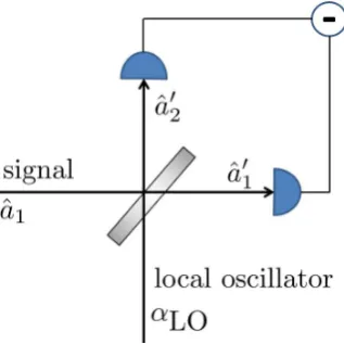
Figure 1.2: The signal is mixed with the local oscillator at a balanced beamsplitter. The pho-tocurrent difference of the outgoing beams is proportional to the quadrature ˆxθwith the phase set
by the local oscillator.
1.4.2 Quantum Optical Measurements
The most important Gaussian measurement in quantum optics is balanced homodyne de-tection [228], which is effectively a measurement of the rotated quadrature ˆxθ = ˆxcosθ−
ˆ
psinθ, where θ = 0 corresponds to the ˆx-quadrature and θ = 3π/2 corresponds to the
p-quadrature. Other values of θ allow any rotated quadrature to be measured. The measurement operators of homodyne detection are projectors onto the required quadra-ture basis, e.g. |xihx|, and the resulting outcome has a probability distribution given by the appropriate marginal distribution of the Wigner function, e.g. P(x) = R
W(x, p)dp. Practically, homodyne detection is realised following the procedure in Fig. 1.2 [1]. The signal state is interfered on a balanced beamsplitter with a coherent laser beam. The laser beam is known as the local oscillator and must be intense enough to give a precise phase reference, and be powerful enough to be treated classically by ignoring the quantum fluc-tuations. After the beamsplitter, the photocurrentsI1 andI2of the outputs are measured
and then subtracted from each other to give the photocurrent differenceI21. It is assumed
that the signal and local oscillator have a fixed phase reference, which is normally a safe assumption since they generally come from the same source, but must be ensured in an experiment. The bosonic operators of the output modes are given by
ˆ
a01 = √1
2(ˆa1−αLO), ˆa 0
2 =
1
√
2(ˆa1+αLO), (1.74) where ˆa1 is the amplitude of the signal and αLO is the complex amplitude of the local
oscillator. The photocurrent differenceI21is proportional to the photon number difference
given by
ˆ
n21= ˆn2−nˆ1=α∗LOaˆ+αLOˆa†. (1.75)
Using the definition of ˆxθ = ˆxcosθ−pˆsinθ from Eq. (1.39) we see that the measured
photocurrent difference I21 is proportional to ˆxθ since it can be shown from the above
equation that
ˆ
n21=
√
2|αLO|xˆθ. (1.76)
A homodyne detector thus measures the quadrature component ˆxθ, where the phase θ is
1.5. Common Experimental Techniques
oscillator. Note that the value of|αLO|can be determined by keeping track of the photon
sum current, which is important since |αLO|is not generally known.
Homodyne measurements are particularly important when restricted to Gaussian quan-tum information theory since any Gaussian measurement can be achieved using only homo-dyne detection, linear optics and Gaussian ancilla modes [78]. One important extension of homodyne detection is heterodyne detection [229]. Heterodyne detection is implemented by first splitting the signal mode on a balanced beamsplitter where the other input is a vacuum mode, then performing homodyne detection on conjugate quadratures at the output [213]. Theoretically, it corresponds to a projection onto coherent states, so the measurement operators areE(α)≡π−1/2|αihα|. Homodyne and heterodyne detection are the most common measurements used in quantum optics with applications ranging from quantum key distribution to quantum state tomography.
1.4.3 Local Quantum Measurements
Often, part of a quantum system is measured to gain information that can be used while further processing the rest of the system. Therefore we need a way to describe the state of a subsystem after the rest of the system has been measured. For Gaussian states, this can be done using covariance matrices by considering a system consisting of two subsystems
A and B, each consisting of an arbitrary number of modes. Here we restrict ourselves to the case where subsystemB has only one mode for simplicity, noting that this result can be generalised to more than one mode in the measured system.
Before measurement, the covariance matrix of the system can be written in block form as in Eq. (1.69), but with the matrix A no longer restricted to be that of a single mode. The state of subsystemA after Gaussian measurement of subsystem B then has a covariance matrix given by [65, 74]
A0 =A−C(B+σ0)−1CT, (1.77)
where σ0 depends on the quantum measurement performed. For an arbitrary Gaussian
measurement,σ0 is the covariance matrix of an arbitrary one-mode pure Gaussian state,
i.e. σ0 =R(θ)diag{λ,1/λ}RT(θ), whereλ≥0 andR(θ) is given in Eq. (1.65). To extend
this to the case of N modes in subsystem B, σ0 should be the covariance matrix of an
arbitrary N-mode pure Gaussian state. Note that the covariance matrix of subsystem
A after the measurement depends only on the type of measurement performed and not on the measurement outcome obtained. In contrast, the displacement vector of the state depends on the outcome of the measurement. Note also, that if subsystemsA and B are uncorrelated, measurement of modeB has no effect on subsystemAas should be expected. For homodyne detection of the x-quadrature of mode B, the corresponding matrix describing the measurement is σ0 withθ= 0 and λ→0. For homodyne detection of the
p-quadrature, θ = π/2 and λ → 0, or equivalently θ = 0 and λ → ∞. For heterodyne detection, θ= 0 and λ= 1. In this way, the state of a subsystem after measurement on the remaining mode can be calculated for the most important Gaussian measurements.
1.5
Common Experimental Techniques
commonly used experimental techniques and the sources of error that can be introduced. In this section, I give a brief summary of some of the most important techniques in modern experimental quantum optics. For a more complete overview, see, for example, [38].
1.5.1 Stokes Operators
Due to their technical convenience, experiments in quantum optics often use Stokes oper-ators, a quantum version of the classical Stokes parameters [196], instead of position and momentum operators. Stokes operators describe continuous variable polarisation states, and are of particular interest since they can be measured by direct detection [132], polar-isation is preserved in free space [103], and it is easy to map polarpolar-isation states to spin states and vice versa [97]. Stokes operators are described by
ˆ
S0= ˆa†xˆax+ ˆa†yˆay, Sˆ1= ˆa†xˆax−ˆa†yˆay
ˆ
S2= ˆa†xˆay+ ˆa†yaˆx, Sˆ3=i(ˆa†yˆax+ ˆa†xˆay),
(1.78)
where ˆax and ˆay are the bosonic annihilation operators describing thex andy orthogonal
polarisation modes. The operator ˆS0commmutes with the other three, and is proportional
to the intensity of the described mode. The other Stokes operators obey the commutation relations
[ ˆSj,Sˆk] =jkl2iSˆl, j, k, l= 1,2,3. (1.79)
Therefore it is impossible to measure simultaneously exact values of any two of these operators. From the commutation relations, the variances of the Stokes operators are bound by the uncertainty relations
ViVj ≥ |hSˆki|2, i6=j6=k, (1.80)
whereVj =hSˆj2i−hSˆji2. Physically, from Eq. (1.78), it can be seen that ˆS1is the operator
for linear polarisation, ˆS2 is the operator for diagonal polarisation, and ˆS3 is the operator
for circular polarisation.
To draw a parallel with the previously introduced position and momentum operators, one can prepare the state with a strong excitation in one of the operators, for example
ˆ
S3, which is the case that will be considered from now on. This means that the state is
circularly polarised, and the ˆS3 operator is essentially classical with|hSˆ3i|2 0, whereas
in contrast hSˆ1i = hSˆ2i = 0. From the relations in Eq. (1.80), it can be seen that the
variance of ˆS3 is unbounded, supporting the idea that it is classical, whereas the variance
of ˆS1 and ˆS2 follow the relationV1V2≥ |hSˆ3i|2. It is often useful to renormalise the Stokes
operators to simplify the uncertainty relation. For a strong excitation of ˆS3, the Stokes
operators are renormalised to [97]
ˆ
S10 ≡ pSˆ1 |S3|
, Sˆ20 ≡ pSˆ2 |S3|
. (1.81)
With the renormalised operators, the uncertainty relation isV10V20≥1. Since this relation has the same form as the Heisenburg uncertainty principle in Eq. (1.25), ˆS1 and ˆS2 can
be thought of as being closely related to the position and momentum quadratures. In addition, the strong excitation of ˆS3 allows the ˆS1- ˆS2 plane (often called the ”dark plane”