Sparse Solutions of Mixed Complementarity Problems

(1)

ISSN Online: 2327-4379 ISSN Print: 2327-4352

DOI: 10.4236/jamp.2020.81002 Dec. 27, 2019 10 Journal of Applied Mathematics and Physics

Sparse Solutions of Mixed Complementarity

Problems

Peng Zhang, Zhensheng Yu

College of Science, University of Shanghai for Science and Technology, Shanghai, China

Abstract

In this paper, we consider an extragradient thresholding algorithm for find-ing the sparse solution of mixed complementarity problems (MCPs). We es-tablish a relaxation l1 regularized projection minimization model for the

original problem and design an extragradient thresholding algorithm (ETA) to solve the regularized model. Furthermore, we prove that any cluster point of the sequence generated by ETA is a solution of MCP. Finally, numerical experiments show that the ETA algorithm can effectively solve the l1

regu-larized projection minimization model and obtain the sparse solution of the mixed complementarity problem.

Keywords

Mixed Complementarity Problem, Sparse Solution, l1 Regularized Projection

Minimization Model, Extragradient Thresholding Algorithm

1. Introduction

Define a continuously differentiable function _{F R}: n_→_Rn_{, and a nonempty set}

{

}

: _{x R a x b}n| ,

Ω = ∈ ≤ ≤

where

a

=

{

R

∪

{ }

−∞

}

n

,

b

=

{

R

∪

{ }

+∞

}

n and a b a<

(

i<b ii, =1,2, , n

)

. The

mixed complementarity problem is to find a vector x∈ Ω_{, such that}

(

) ( )

T

0, .

y x F x− ≥ ∀ ∈ Ωy

(1) The mixed complementarity problem, also known as box constrained varia-tional inequality problem, denoted by MCP (a, b, F). In particular, if : _Rn

+ Ω = , the mixed complementarity problem becomes a nonlinear complementarity prob-lem (NCP), is to find a vertor x≥0, such that

( )

T

0, 0.

F x ≥ F x x=

How to cite this paper: Zhang, P. and Yu, Z.S. (2020) Sparse Solutions of Mixed Com-plementarity Problems. Journal of Applied Mathematics and Physics, 8, 10-22. https://doi.org/10.4236/jamp.2020.81002

Received: November 28, 2019 Accepted: December 24, 2019 Published: December 27, 2019

http://creativecommons.org/licenses/by/4.0/

(2)

DOI: 10.4236/jamp.2020.81002 11 Journal of Applied Mathematics and Physics Moreover, if F x

( )

:=Mx q+ , where _{M R}_∈ n n× ,_{q R}_∈ n_{, the nonlinear} com-plementary problem reduces a linear comcom-plementary problem (LCP):

(

)

T

0, 0, 0.

x≥ Mx q+ ≥ Mx q x+ =

The set of solution to the mixed complementarity problem is denoted by SOL

(F), throughout this paper, we assume SOL F

( )

≠ ∅.

The MCP has wide applications in fields of science and engineering [1] [2], and many results on its theories and algorithms have been developed (see e.g. [3] [4] [5] [6]).

In recent years, the problem of recovering an unknown sparse solution from some linear constraints has been an active topic with a range of applications in-cluding signal processing, machine learning, and computer vision [7], and there are many articles available for sloving the sparse solutions of systems of linear equations [8]-[13] as well as the optimization problems [14] [15] [16].

In contrast with the fast development in sparse solutions of optimization and linear equations, there are few researches available for the sparse solutions of the complementarity problems. The sparse solution problem of linear complementar-ity was first studied by Chen and Xiang [17], by using the concept of minimum

(

0 1

)

p < <p norm solution, they studied the characteristics and calculations of sparse solutions and minimum p-norm solutions for linear complementarity problems. Recently, some solution methods had been proposed for LCP and NCP, for examples, shrinkage-thresholding projection method [18], half thre-sholding projection algorithm [19] and extragradient thresholding method [20].

Along with the research of [17] [18] [19] [20], in this paper, we aim to design an extragradient thresholding Algorithm for the sparse solution of MCP, and which can be seen as an extension of the sparse solution algorithm for NCP.

Due to the relationship between MCP and the variational inequality, we aim to seek a vector x∈ Ω_{by solving the solution of} l₀ norm minimization problem:

(

) ( )

0

T

min ,

s.t. 0,

x

y x F x− ≥

(2)

for any y∈ Ω, where x0 stands for the number of nonzero components of x

and a solution of problem (2) is called the sparse solution of MCP.

In essence, the minimization problem (2) is a sparse optimization problem with equilibrium constraints. It is not easy to get solutions due to the equili-brium constraints, even if the objective function is continuous.

To overcome the difficulty for the l0 norm, many researchers have suggested

to relax the l0 norm and instead to consider the l1 norm, see [21]. Motivated

by this outstanding work, we consider applying l1 norm minimization to find

the sparse solution of MCP, and we obtain the following minimization problem to approximate problem (2):

(

) ( )

1

T

min ,

s.t. 0

x x

y x F x

∈Ω

− ≥

(3)

DOI: 10.4236/jamp.2020.81002 12 Journal of Applied Mathematics and Physics for any y∈ Ω_{and where} ₁

1

n i i

x x

= =

∑

_.

Given a vector x∈ Ω_{, let} P xΩ

( )

be the projection of x on Ω, for conven-ience, we write P xΩ

( )

=

[ ]

xΩ, it is well known (see, e.g., [22]) that

*

x is a solu-tion point of problem (1) if and only if it satisfies the following projecsolu-tion equa-tion:

( )

* _: * *

( )

* _0,

W x x x F x

Ω

 

= −_ − _ =

(4) and therefore problem (3) is equivalent to the following optimization problem

( )

1 ,

min :

s.t. .

n

x z R f x x

x x F x ∈

Ω =

=_ − _

(5)

In order to simplify the objective function, we introduce a new variable n

z R∈ _{and a regularization parameter}λ >0_{and establish the corresponding}

regularized minimization problem as follows:

( )

2

1 ,

min , :

s.t. .

n

x z R f x z x z x

z x F x

λ λ

∈

Ω = − + =_ − _

(6)

We call (6) the l1 regularized projection minimization problem.

This paper is organized as follows. In Section 2, we study the relation between the solution of model (6) and that of problem (3), and we show theoretically that (6) is a good approximation of problem (3). In Section 3, we propose an extra-gradient thresholding algorithm(ETA) for (6) and analyze the convergence of this algorithm. Numerical results are given in Section 4 and conclusion is de-scribed in Section 5.

2. The

l

1

Regularized Approximation

In this section, we study the relation between the solution of model (6) and that of model (3). The following theorem shows that model (6) is a good approxima-tion of problem (3).

Theorem 2.1. For any fixed λ >0_,_{the solution set of}₍₆₎_{is nonempty and}

bounded. Let

{

(

x zλ_k, λ_k

)

}

be a solution of (6), and

{ }

λk be any positive

se-quence converging to 0. If SOL F

( )

≠ ∅, then

{

(

x zλ_k, λ_k

)

}

has at least one

ac-cumulation point, and any accumulation point x∗_of

{ }

k

xλ is a solution of

(1.3).

Proof. For any fixed λ >0_{, since}

( )

, as

( )

, ,

f x zλ → +∞ x z → ∞ (7) which means f x zλ

(

,

)

is coercivity. On the other hand, it is clear that for any

n

x R∈ _and _{z R}_∈ n_, _{f x z}

_{( )}

_, ₀

λ ≥ . This together with (7) implies the level set

( )

(

)

( )

{

, n n| , 0, 0 and

}

(4)

DOI: 10.4236/jamp.2020.81002 13 Journal of Applied Mathematics and Physics is nonempty and compact, where x0∈Rn and z0 =x F x0−

( )

0 _Ω are given

points, which deduces that the solution set of problem (6) is nonempty and bounded since f x zλ

(

,

)

is continuous on L.

Now we consider the proof of the second part of this theorem. Let

( )

ˆ

x SOL F∈ and zˆ=_x F xˆ−

( )

ˆ __Ω_{. from (5), we have} x zˆ ˆ= . Since

(

x z

λ_k

,

λ_k

)

is a solution of (6) with λ λ= k, where zλk =xλk −F x

( )

λk _Ω, it follows that

{

2

}

2

1 1

2

1

max ,

ˆ ˆ ˆ

ˆ .

k k k k k k k k

k

x z x x z x

x z x

x

λ λ λ λ λ λ λ λ

λ λ

− ≤ − +

≤ − + =

(8)

This implies that for any λ >k 0,

1 1 ˆ .

k

xλ ≤ x

(9) Hence the sequence

{ }

x

λ_k is bounded and has at least one cluster point and so is

{ }

z

λ_k due to

2

1

ˆ

k k k

xλ −zλ ≤

λ

x .

Let x∗_and _z∗_{be any cluster points of}

{ }

k

x

λ and

{ }

z

λ_k , respectively, and

( )

k k k

zλ =_xλ −F xλ __Ω. Then there exists a subsequence of

{ }

λk , say

{ }

λkj , such that

lim _k and lim _k .

j j

k xλ x k zλ z

∗ ∗

→∞ = →∞ =

We can obtain z∗ x F x∗

( )

∗ Ω

 

=_ − _ _{by letting} k_j → ∞_in

( )

k k k

zλ =_xλ −F xλ __Ω. Letting λk_j →0, in

2

1

ˆ

kj kj kj

xλ −zλ ≤

λ

x

yields x∗ ₌z∗_{. Consequently,} _x∗ _{x F x}∗

( )

∗ Ω

 

=_ − _ _{, which implies} x∗_∈SOL F

( )

_. Let kj tend to ∞ in (9), we get x ₁ xˆ1

∗ _≤ _{. Then by the arbitrariness of}

( )

ˆ

x SOL F∈ , we know x∗_{is solution of problem (3). This completes the proof.}_

3. Algorithm and Convergence

In this section, we give the extragradient thresholding algorithm (ETA) to solve

1

l regularization projection minimization problem (6) and give the convergence analysis of ETA.

First, we review some basic concepts about the monotone operator and the properties of the projection operator which can be found in [23].

Lemma 3.1. Let PK

( )

⋅ be a projection from Rn to K, where K is a non-

empty closed convex subset on _Rn_._{Then we have} (a) For _{y R}_∈ n_,

[ ]

(

)

T

(

[ ]

)

0, ;

K K

y P y− P y x− ≥ ∀ ∈x K

(10)

(5)

DOI: 10.4236/jamp.2020.81002 14 Journal of Applied Mathematics and Physics

[ ]

2

(

)

T

(

[ ]

)

_.

K K K K

P y P z

−

≤

y z

−

P y P z

−

(11) Using Lemma 3.1, we can obtain the following properties easily.

Lemma 3.2. Define a residue funtion

( )

:

[

]

, 0, n.

K

H

α

=P x−

α

d

α

≥ d R∈

(12)

Then the following statements are valid.

(a) For any α ≥0, x H−

_α

( )

α

is non-increasing;

(b) ∀ >α 0_,

(

( )

)

( )

2

T x H

d x H α α

α

−

− ≥ ;

(c) _{∀ ∈}_{z R}n_,

[ ]

2 2

[ ]

2

K K

P z x

−

≤ −

z x

−

P z z

−

_.

In this paper, we suppose the mapping _{F R}: n_→_Rn_{is co-coercive on the set}

Ω, i.e., there exists a constant c>0_{such that}

( )

2

, , , .

F x F y x y− − ≥c F x F y− ∀x y∈ Ω

It is clear that the co-coercive mapping is monotone, namely,

( )

, 0, , .

F x −F y x y− ≥ ∀x y∈ Ω For a given _zk _{∈ Ω}_and ₀

k

λ > _{, we consider an unconstrained}

minimiza-tion subproblem:

( )

2

1

min_n _k , k : k .

k

x R∈ fλ x z = x z− +λ x (13) Evidently, the minimizer _x*_{of the model (13) satisfies the corresponding}

optimality condition

( )

* _,

k

x =S zλ (14)

where the shrinkage operator Sλ is defined by (see, e.g., [18])

( )

(

)

, ;

2 2

0, ;

2 2

, .

2 2

i i

z z

S z z

z z

λ

λ λ

 − ≥

  

=_ − ≤ ≤

 

+ ≤ −



(15)

It demonstrates that a solution _{x R}_∈ n_{of the subproblem (13) can be}

analyt-ically expressed by (14).

In what follows, we construct the extragradient thresholding algorithm (ETA) to solve the l1 regularized projection minimization problem (6).

Algorithm ETA

Step 0: Choose 0

( )

0

0≠z ∈ Ω, ,λ γ >0, , ,τ µl ∈ 0,1 ,>0 and a positive integ-ers nmax >K0>0, set k=0.

Step 1: Compute k _k

( )

k , k k

( )

k k

x =S zλ y =_x −

α

F x __Ω, where αk=γlmk with

k

(6)

( ) ( )

.

k k

k

x y

F x F y

µ

α

−

− ≤

(16) Step 2: If xk−zk ≤ or the number of iterations is greater than nmax, then

return _{z x y}k, ,k k_{and stop. Otherwise, compute}

( )

1 _,

k k k

k

z + x

α

F y

Ω

 

=_ − _

and update λk+1 by

0 1

, if 1is a multiple of ,

, otherwise.

k k

k

k K

τλ

λ

+

+ 

=  

Step 3: Let k k= +1, then go to Step 1. Define

( )

, 0

x α =_x−αF x __Ω α ≥ and

( )

,

( ) (

, ,

)

(

,

)

e x a = −x x α r xα = e xα

It is easy to see that _xk_{is a solution for}_MCP_{if and only if}

(

k,

)

0, 0 e x

α

= ∀ >

α

_.

The following lemma plays an important role in the analysis of the global convergence of the Algorithm ETA.

Lemma 3.3. Suppose that mapping F is co-coercive and SOL F

( )

≠ ∅. If _xk

generated by ETA is not a solution of MCP F

( )

, then for any x SOL Fˆ∈

( )

, we have

( )

(

)

2

ˆ

, , 1 .

k k

k k k k k x y

F y x x F y x y µ

γ

−

− ≥ − ≥ −

(17) Proof. Since x SOL Fˆ∈

( )

and _yk_{∈ Ω}_{, it follows that} _{F x y}

( )

_ˆ _, k₋_x_ˆ _≥₀_. By the co-coercive of mapping F, we have

_{F y}

( )

k

,

_y

k

₋

_x

ˆ

_≥

0

_{. Hence}

( )

( ) ( )

2 2

2

ˆ ˆ

, ,

,

, ,

1

1 _,

k k k k k k

k k k

k k k k k k k

k k k k

k k

F y x x F y x y y x F y x y

F x x y F x F y x y

x y x y

x y

µ

α α

µ γ

− = − + −

≥ −

= − − − −

≥ − − −

−

≥ −

where the second inequality comes from Lemma 3.2(b) and (16), and the last inequality is based on αk ≤γ.

The following theorem gives the global convergence of the algorithm ETA. Theorem 3.4. Suppose F is co-coercive and SOL F

( )

≠0. If

{ }

_xk _and

{ }

_yk _{are infinite columns generated by the algorithm ETA}_,_then

lim k k 0.

(7)

DOI: 10.4236/jamp.2020.81002 16 Journal of Applied Mathematics and Physics Further,

{ }

xk converges to a solution of the problem MCP(a, b, F).

Proof. Let x SOL Fˆ∈

( )

, by Lemma 3.2(c) and (17), we have

( )

(

)

( )

( ) (

)

( ) (

)

( ) (

)

( )

(

)

(

)

2 1

2 ₁ 2

T T

2 ₁ ₁2

T

2 ₁ ₁2

T

2 2 ₁ 2 ₁

ˆ

ˆ 2 ˆ 2

ˆ 2

k

k k k k k

k k

k k k k k k k k

k k

k k k k k k

k

k k k k k k k k k k

k

z x

x F y x z x F y

x x F y x x F y z x x z

x x F y z y x z

x x x y z y x y F y z y

α

+ + + + + + + + − ≤ − − − − + = − − − − − − − ≤ − − − − − = − − − − − + − − − (19)

Now consider the last term of Equation (19), by Lemma 3.1 (a), we have

( )

(

)

T

(

₁

)

0

k k k k k

k

y ₋x ₊α F x z + ₋y _≥ It follows that

( )

(

)

(

)

( )

(

)

(

)

(

( )

)

(

)

( ) ( )

(

)

(

)

( ) ( )

(

)

T ₁

T ₁ T ₁

T ₁ 2 2 2 1 2 2 2 2

k k k k k

k

k k k k k k k k k k

k k

k k k k

k

k k k k

k

x y F y z y

x y F y z y y x F x z y

F x F y z y

α α α α α + + + + + − − − ≤ − − − + − + − = − − ≤ − + − (20)

Replacing (20) into (19), and by (16), we deduce

( ) ( )

(

)

(

)

2 2 2 2

1 1

2 ₂

2 1

2 2 ₂ 2

2 ₂ 2

ˆ ˆ

ˆ

ˆ 1

k k k k k k

k k k k

k

k k k k k

k k k

z x x x x y z y

F x F y z y

x x x y x y

x x x y

α µ µ + + + − ≤ − − − − − + − + − ≤ − − − + − = − − − − (21)

According to the definition of shrinkage operator (15), we know that

1 _ˆ 1 _{ˆ .}

k k

x + _{− ≤}x z + ₋x

Hence,

{

_xk ₋_xˆ 2

}

_{has contraction properties, which means}

{ }

_xk _{is bounded,}

and

(

₂

)

2

{

2 ₁ 2

}

0 0

ˆ ˆ

1 k k k k ,

k x y k x x x x

µ

∞ ∞ +

= =

−

∑

− ≤

∑

− − − < +∞

so we get (18) holds.

Since

{ }

_xk _{is bounded, the sequence}

{ }

_xk _{has at least one cluster point, let}

*

x be a cluster points of

{ }

_xk _{and a subsequence}

{ }

x

ki _{converge to} _x*_{. Next}

we will show _x*_∈_{SOL F}

( )

_{, we consider two cases:}

Case 1: assume that there is a positive low bounded αmin such that

min 0

i k

α ≥α > , then by inequality

{ } ( )

( )

{ } ( )

min 1,

α

e x,1 ≤ e x,

α

≤max 1,

α

e x,1 .

(8)

DOI: 10.4236/jamp.2020.81002 17 Journal of Applied Mathematics and Physics the continuity of e x

(

,α

)

for x and (18), we get

( )

(

_{{ }}

)

(

)

{

}

{

}

* min min ,

,1 lim ,1 lim

min 1, ,

lim lim 0.

min 1, min 1,

i i i

i i

i

i i i

i i i k k k k k k

k k k

k

k k

e x

e x e x

e x x y

α α α α α →∞ →∞ →∞ →∞ = ≤ − ≤ = =

Case 2: assume αk_i →0, for enough large ki, by the Lemma 3.2 (a) and the

Arimijo search (16), we get

( )

1 ,

1

,1 ₁ .

i i

i i i

i

i k

k

k k k

k k

e x l

e x F x F x

l l

α

µ µ α

α

 

  _ _ __

 

≤ < _{− } _ __

 

Hence, we have

( )

*_,1 _lim

( )

i_,1 _lim

( )

i i 1 _0. i

i i

k k k

k

k k

e x e x F x F x

lα

→∞ →∞

  

= ≤ − _ _ __ =

 

  (23)

In summary, we can get _x*_∈_{SOL F}

( )

_{. Replacing this formula into (21), we}

have

(

)

2 2 2 2

1 * 1 * *

₁

2

_.

k k k k k

x

+

₋

x

_≤

z

+

₋

x

_≤

x

₋

x

_{− −}

µ

x

₋

y

Hence we get

{ }

_xk _{converges to the solution} _x*_{. The proof is thus}

com-plete. 

4. Numerical Experiments

In this section, we present some numerical experiments to demonstrate the ef-fectiveness of our ETA algorithm, and show the algorithm can obtain the sparse solution of the MCP (a, b, F).

We will stimulate three examples to implement the ETA algorithm. They will be ran 100 times for difference dimensions, and thus average results will be recorded. In each experiment, we set _z0 ₌_e_, _γ ₌₂_c_, _l₌_0.1_, _{µ =}₁_c_,

max 2000

n =

and other related parameters will be given in the following test example.

4.1. Test for LCPs with Z-Matrix [18]

The test is associated with the Z-matrix which has an important property, that is, there is a unique sparse solution of LCPs when M is a kind of Z-matrix. Let us consider LCP(q, M) where

T

1 1 1

1

1 ₁ 1 1

1

1 1 ₁ 1

n

n n n

M I ee n n n

n

n n n

(9)

DOI: 10.4236/jamp.2020.81002 18 Journal of Applied Mathematics and Physics and

T

1 _{1, , ,}1 1 q

n n n

 

=_ − _

  , here In is the identity matrix of order n and

(

)

T

1,1, ,1 n

e= ∈R . Such a matrix M is widely used in statistics. It is clear that

M is a positive semidefinite Z-matrix. For any scalar α ≥0, we know that vector

1

x=αe e+ _{is a solution to LCP(}_q_,_M_{), since it satisfies}

(

)

T 1

0, 0, 0.

x≥ Mx q Me q+ = + = x Mx q+ =

Among all the solution, the vector x eˆ= =1

(

1,0, ,0

)

T is the unique sparse

solution.

We choose _z0 ₌_e_, _c₌₁_,

0 0.2

λ = , γ =2c, τ =0.75, l=0.1, µ =1c,

1 6e = −

 , nmax=2000, K0=5. We will take advantage of the recovery error

ˆ

x x− to evaluate our algorithm. Apart from that, the average cpu time (in seconds), the average number of iteration times and residual x z− will also be taken into consideration on judging the performance of the method.

As indicated in Table 1, the ETA algorithm behaves very robust because the average number of times of iteration is identically equal to 205, the recovered error x x−ˆ and residual x z− are basically similar. In addition, the spar-sity x₀ of the recovered solution x is in all cases equivalents to 1, which means the recover is successful.

4.2. Text for LCPs with Positive Semidefinite Matrices

In this subsection, we test ETA for randomly created LCPs with positive semide-finite matrices. First, we state the way of constructing LCPs and their solution. Let a matrix _{Z R}_∈ n r×

(

_{r n}_<

)

_{be generated with the standard normal} distribu-tion and _{M ZZ}₌ T_{. Let the sparse vector} _x_ˆ_{be produced by choosing randomly}

the s=0.01∗n_{nonzero components whose values are also randomly generated} from a standard normal distribution. After the matrix M and the sparse vector

ˆ

x have been generated, a vector _{q R}_∈ n_{can be constructed such that} _x_ˆ_{is a} solution of the LCP (q, M). Then xˆ can be regarded as a sparse solution of the LCP (q, M). Namely,

(

)

T

0

ˆ 0, ˆ 0, ˆ ˆ 0, and ˆ 0.01 .

x≥ Mx q+ ≥ x Mx q+ = x = ∗n

[image:9.595.207.539.594.734.2]

To be more specific, if xˆi >0 then choose qi = −

( )

Mxˆ i, if xˆi=0 then

Table 1. ETA’s computational results on LCPs with Z-matrices.

n Iter x x−ˆ x z− xˆ₀ x0 Time(sec.)

3000 205 7.7007E−06 7.5424E−07 1 1 2.89

5000 205 7.6995E−06 7.5424E−07 1 1 7.92

10,000 205 7.6986E−06 7.5424E−07 1 1 36.68

15,000 205 7.6983E−06 7.5424E−07 1 1 78.40

20,000 205 7.6981E−06 7.5424E−07 1 1 148.45

(10)

DOI: 10.4236/jamp.2020.81002 19 Journal of Applied Mathematics and Physics choose q_i =

( ) ( )

Mxˆ _i − Mxˆ _i_{. Let}_M_and_q_{be the input to our ETA algorithm and}

take _z0 ₌_e _, _c₌_max

(

_{svd M}

( )

)

_,

0 0.2

λ = _, γ =2c _, τ =0.75 _, l=0.1 ,

1c

µ = , =1 10e− , nmax=2000, K0=max 2, 10000

(

 n

)

, here 10000 n

denotes the largest integer less than 10,000/n. Then ETA will output a solution x. Similarly, the average number of iteration times, average cpu time (in seconds), and the residual x z− will also be taken into consideration on valuating our ETA algorithm.

As manifested in Table 2, the ETA algorithm performs quite efficiently. Fur-thermore, the sparsity x ₀ of recovered solution x is in all cases equal to the sparsity xˆ₀, which means the recover is exact.

4.3. Test for Co-Coercive Mixed Complementarity Problem

We now consider a co-coercive mixed complementarity problem (MCP) with

( )

F x =D x +Mx q+

₍₂₄₎ where D x

( )

and Mx q+ are the nonlinear part and the linear part of F x

( )

, generate a linear part of Mx q+ _{in a way similar to}_[24]_{. The matrix}

T

M A A B= + , where A is an n n× matrix whose entries are randomly gener-ated in the interval

(

−5,5

)

, and a skew-symmetric matrix B is generated in the same way. In D x

( )

, the nonlinear part of F x

( )

, the components are

( )

arctan

( )

j j j

D x =d ∗ x _{, and}d_j is a random variable in

(

−1,0

)

, see similar example [25]. Then the sequent part of generating the sparse vector xˆ and vector _{q R}_∈ n_{such that}

(

) ( )

T

0

ˆ , ˆ ˆ 0, , and ˆ 0.01 .

x∈ Ω y x F x− ≥ ∀ ∈ Ωy x = ∗n

is similar to the procedure of Section 4.2. Let M and q be the input to our ETA algorithm and take _z0 ₌_e_, _c₌_{150 log}_∗

_{( )}

_n _,

0 0.2

λ = _, γ =2c_, τ =0.75_, 0.1

l= , µ =1c_, =1 6e− , nmax =2000, K0=max 2,10000

(

n

)

, and

( )

,1

d = −rand n . Then ETA will output a solution x. Similariy, the average num-ber of iteration times, the average residual x z− , the average sparsity x0 of

x, and the average cpu time (in seconds) will also be taken into consideration on valuation our ETA algorithm.

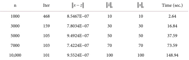
It is not difficult to see from Table 3 that the ETA algorithm also performs quite efficiently in such mixed complementarity problems. The sparsity x0 of the

[image:10.595.206.540.617.733.2]

re-covered solution x are all equal to the sparsity xˆ0, that is, the recover is exact.

Table 2. Results on randomly created LCPs with positive semidefinite matrices.

n Iter x z− xˆ₀ x₀ _{Time (sec.)}

2000 350 8.0136E−11 20 20 18.05

3000 210 9.8366E−11 30 30 11.86

4000 142 8.5188E−11 40 40 28.65

5000 142 9.5243E−11 50 50 20.47

(11)

[image:11.595.208.540.91.196.2]

Table 3. Results on co-coercive mixed complementarity problems.

n Iter x z− xˆ₀ x₀ _{Time (sec.)}

1000 468 8.5467E−07 10 10 2.64

3000 159 7.8034E−07 30 30 16.84

5000 105 9.4924E−07 50 50 37.59

7000 103 7.4224E−07 70 70 73.59

10,000 101 9.5524E−07 100 100 148.94

5. Conclusion

In this paper, we concentrate on finding sparse solution for co-coervice mixed complementarity problems (MCPs). An l1 regularized projection minimization

model is proposed for relaxation, and an extragradient thresholding algorithm (ETA) is then designed for this regularized model. Furthermore, we analyze the convergence of this algorithm and show any cluster point of the sequence gener-ated by ETA is a sparse solution of MCP. Preliminary numerical results indicate that the l1 regularized model as well as the ETA is promising to find the spare

solution of MCPs.

Data Availability

Since data in the Network Vector Autoregression (NAR) is not public, we have not done empirical analysis.

Acknowledgements

This paper is supported by the Top Disciplines of Shanghai.

Conflicts of Interest

The authors declare no conflicts of interest regarding the publication of this pa-per.

References

[1] Ferris, M.C. and Pang, J.S. (1997) Engineering and Economic Applications of Com-plementarity Problem. SIAM Review, 39, 669-713.

https://doi.org/10.1137/S0036144595285963

[2] Harker, P.T. and Pang, J.S. (1990) Finite-Dimensional Variational Inequality and Nonlinear Complementarity Problems: A Survey of Theory, Algorithms and Appli-cations. Mathematical Programming, 48, 161-220.

https://doi.org/10.1007/BF01582255

[3] Billups, S.C., Dirkse, S.P. and Ferris, M.C. (1997) A Comparison of Algorithms for Large-Scale Mixed Complementarity Problems. Computational Optimization and Applications, 7, 3-25.https://doi.org/10.1007/978-0-585-26778-4_2

(12)

DOI: 10.4236/jamp.2020.81002 21 Journal of Applied Mathematics and Physics [5] Facchinei, F. and Pang, J.S. (2003) Finite-Dimensional Variational Inequality and

Complementarity Problems II. Springer Series in Operations Research, Springer, New York.https://doi.org/10.1007/b97544

[6] Zhou, Z.Y. and Peng, Y.C. (2019) The Locally Chen-Harker-Kanzow-Smale Smooth-ing Functions for Mixed Complementarity Problems. Journal of Global Optimiza-tion, 74, 169-193.https://doi.org/10.1007/s10898-019-00739-4

[7] Eldar, Y.C. and Kutyniok, G. (2012) Compressed Sensing: Theory and Applications. Cambridge University Press, Cambridge.

[8] Bruckstein, A.M., Donoho, D.L. and Elad, M. (2009) From Sparse Solutions of Sys-tems of Equations to Sparse Modeling of Signals and Images. SIAM Review, 51, 34-81.https://doi.org/10.1137/060657704

[9] Candes, E.J., Romberg, J. and Tao, T. (2006) Robust Uncertainty Principles: Exact Signal Reconstruction from Highly Incomplete Frequency Information. IEEE Trans-actions on Information Theory, 52, 489-509.

https://doi.org/10.1109/TIT.2005.862083

[10] Candes, E. and Tao, T. (2005) Decoding by Linear Programming. IEEE Transac-tions on Information Theory, 51, 4203-4215.

https://doi.org/10.1109/TIT.2005.858979

[11] Foucart, S. and Rauhut, H. (2013) A Mathematical Introduction to Compressive Sensing. Springer, Basel.https://doi.org/10.1007/978-0-8176-4948-7

[12] Ge, D., Jiang, X. and Ye, Y. (2011) A Note on the Complexity of Lp Minimization. Mathematical Programming, 129, 285-299.

https://doi.org/10.1007/s10107-011-0470-2

[13] Natarajan, B. (1995) Sparse Approximate Solutions to Linear Systems. SIAM Jour-nal on Computing, 24, 227-234.https://doi.org/10.1137/S0097539792240406 [14] Chen, X., Xu, F. and Ye, Y. (2010) Lower Bound Theory of Nonero Entries in

Solu-tions of l2−lp Minimization. SIAM Journal on Scientific Computing, 32, 2832- 2852.https://doi.org/10.1137/090761471

[15] Beck, A. and Eldar, Y. (2013) Sparsity Constrained Nonlinear Optimization: Opti-mality Conditions and Algorithms. SIAM Journal on Optimization, 23, 1480-1509.

https://doi.org/10.1137/120869778

[16] Lu, Z. (2014) Iterative Hard Thresholding Methods for l0 Regularized Convex Cone Programming. Mathematical Programming, 147, 125-154.

https://doi.org/10.1007/s10107-013-0714-4

[17] Chen, X. and Xiang, S. (2016) Sparse Solutions of Linear Complementarity Prob-lems. Mathematical Programming, 159, 539-556.

https://doi.org/10.1007/s10107-015-0950-x

[18] Shang, M. and Nie, C. (2014) A Shrinkage-Thresholding Projection Method for Sparsest Solutions of LCPs. Journal of Inequalities and Applications, 2014, Article No. 51.https://doi.org/10.1186/1029-242X-2014-51

[19] Shang, M., Zhang, C., Peng, D. and Zhou, S. (2015) A Half Thresholding Projection Algorithm for Sparse Solutions of LCPs. Optimization Letters, 9, 1231-1245.

https://doi.org/10.1007/s11590-014-0834-7

[20] Shang, M., Zhou, S. and Xiu, N. (2015) Extragradient Thresholding Methods for Sparse Solutions of Co-Coercive NCPs. Journal of Inequalities and Applications, 2015, Article No. 34. https://doi.org/10.1186/s13660-015-0551-5

(13)

DOI: 10.4236/jamp.2020.81002 22 Journal of Applied Mathematics and Physics 795-814.https://doi.org/10.1007/s10957-014-0549-z

[22] Gabriel, S.A. and More, J.J. (1997) Smoothing of Mixed Complementarity Problems in Complementarity and Variational Problems.

[23] Zarantonello, E.H. (1971) Projections on Convex Sets in Hilbert Space and Spectral Theory. In: Zarantonello, E.H., Ed., Contributions to Nonlinear Functional Analy-sis, Academic Press, New York.

[24] Harker, P.T. and Pang, J.S. (1990) A Damped-Newton for the Linear Complemen-tarity Problems. In: Allgower, E.L. and Georg, K., Eds., Computational Solution of Nonlinear Systems of Equations: AMS Lectures on Applied Mathematics, 26th Edi-tion, American Mathematical Society, Providence, 265-284.