Compressive sensing for sparse approximations: constructions, algorithms, and analysis

(1)

Constructions, Algorithms, and Analysis

Thesis by

Weiyu Xu

In Partial Fulfillment of the Requirements for the Degree of

Doctor of Philosophy

California Institute of Technology Pasadena, California

2010

(2)

c

2010

(3)

Acknowledgements

I thank my advisor Professor Babak Hassibi for his guidance and support throughout my PhD study at Caltech. His great passion and capability for fundamental theoret-ical research over a broad spectrum of fields have been, and will always be, a great inspiration to me. It is a great pleasure and privilege for me to have worked together with him over the past four years. He was always available to help work out the problems whenever I was stuck in research. His nice personality has made me feel at home at Caltech even though my motherland is thousands of miles away.

I thank Professor Emmanuel Cand`es for introducing me to his seminal work on the magic of ℓ1 minimization in a homework set when I was a first-year Caltech

graduate student taking his course ACM 103. It was hard to imagine then that this homework problem, together with a little bit curiosity of my own, would attract me to the beautiful topics in compressive sensing and would eventually lead to the completion of this thesis. Professor Cand`es’s encouragement and support have been a very valuable part of my graduate study.

My special thanks go to my other collaborators besides my advisor, Mihailo Sto-jnic, Ben Recht, M. Amin Khajehnejad, Salman Avestimehr, Alex Dimakis, Sina Ja-farpour, Morten Hansen, and Robert Calderbank, without whom some of the chapters in this thesis would not have been possible. I have been learning a lot through the collaborations. I would especially like to acknowledge that Professor Rolf Schneider very kindly mailed to me his paper on random projections of polytopes when I could not find it in the library.

(4)

committees and providing valuable feedback.

I am grateful to Shirley for her pleasant and efficient help over the last four years. It has always been fun to hang out in Moore 155 and collaborate on research with the labmates. The friendship and the enormous fun of working there are just hard to express in a single page. Amir Farajidana, Radhika Gowaikar, Vijay Gupta, Yindi Jing, Devdutt Marathe, Michela Munoz-Fernandez, Fr´ed´erique Oggier, Farzad Parvaresh, Chaitanya Rao, Masoud Sharif, Mihailo Stojnic, Sormeh Shadbakht and Haris Vikalo all have set up very good role models and guided me through the happy days at the Institute, and I enjoy interacting with them very much. I am especially thankful towards Chaitanya Rao, who, on my first day in Pasadena, spared his Friday evening and took me to a dinner at a Thai restaurant on the Colorado Boulevard. The delicious food there had me deeply attracted to this beautiful sunny place.

I would also like to thank many friends of mine outside Caltech, who have helped me and made my life more fun.

(5)

Abstract

Compressive sensing is an emerging research field that has applications in signal processing, error correction, medical imaging, seismology, and many more other areas. It promises to efficiently recover a sparse signal vector via a much smaller number of linear measurements than its dimension. Naturally, how to design these linear measurements, how to construct the original high-dimensional signals efficiently and accurately, and how to analyze the sparse signal recovery algorithms are important issues in the developments of compressive sensing. This thesis is devoted to addressing these fundamental issues in the field of compressive sensing.

In compressive sensing, random measurement matrices are generally used and ℓ1

minimization algorithms often use linear programming or other optimization methods to recover the sparse signal vectors. But explicitly constructible measurement ma-trices providing performance guarantees were elusive andℓ1 minimization algorithms

are often very demanding in computational complexity for applications involving very large problem dimensions. In chapter 2, we propose and discuss a compressive sens-ing scheme with deterministic performance guarantees ussens-ing deterministic explicitly constructible expander graph-based measurement matrices and show that the sparse signal recovery can be achieved with linear complexity. This is the first of such a kind of compressive sensing scheme with linear decoding complexity, deterministic performance guarantees of linear sparsity recovery, and deterministic explicitly con-structible measurement matrices.

The popular and powerful ℓ1 minimization algorithms generally give better

(6)

signal recovery accuracy, using high-dimensional geometry, we give a unified null-space Grassmann angle-based analytical framework for compressive sensing. This new framework gives sharp quantitative trade-offs between the signal sparsity and the recovery accuracy of the ℓ1 optimization for approximately sparse signal. Our

results concern the fundamental “balancedness” properties of linear subspaces and so may be of independent mathematical interest.

The conventional approach to compressed sensing assumes no prior information on the unknown signal other than the fact that it is sufficiently sparse over a particu-lar basis. In many applications, however, additional prior information is available. In chapter 4, we will consider a particular model for the sparse signal that assigns a prob-ability of being zero or nonzero to each entry of the unknown vector. The standard compressed sensing model is therefore a special case where these probabilities are all equal. Following the introduction of thenull-space Grassmann angle-based analytical framework in this thesis, we are able to characterize the optimal recoverable sparsity thresholds using weighted ℓ1 minimization algorithms with the prior information.

The roles ofℓ1minimization algorithm in recovering sparse signals from incomplete

measurements are now well understood, and sharp recoverable sparsity thresholds for

ℓ1 minimization have been obtained. The iterative reweighted ℓ1 minimization

algo-rithms or related algoalgo-rithms have been empirically observed to boost the recoverable sparsity thresholds for certain types of signals, but no rigorous theoretical results have been established to prove this fact. In chapter 5, we try to provide a theoretical foun-dation for analyzing the iterative reweighted ℓ1 algorithms. In particular, we show

that for a nontrivial class of signals, the iterative reweighted ℓ1 minimization can

in-deed deliver recoverable sparsity thresholds larger than the ℓ1 minimization. Again,

(7)

(8)

List of Figures

2.1 A bipartite graph . . . 24

2.2 (k, ǫ) vertex expander graph . . . 41

2.3 Progress lemma . . . 46

2.4 Gap elimination lemma . . . 48

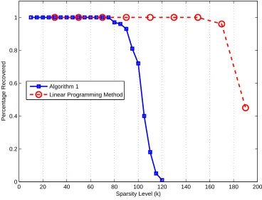
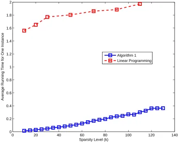
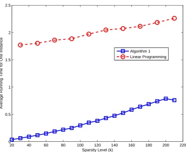
2.5 The probability of recovering ak-sparse signal withn= 1024 andm = 512 59 2.6 The average running time (seconds) of recovering a k-sparse signal with n = 1024 andm = 512 . . . 60

2.7 The probability of recovering ak-sparse signal withn= 1024 andm = 640 61 2.8 The average running time (seconds) of recovering a k-sparse signal with n = 1024 andm = 640 . . . 62

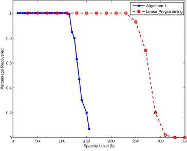
2.9 The probability of recovering a k-sparse signal with n = 2048 and m= 1024 . . . 63

2.10 The average running time (seconds) of recovering a k-sparse signal with n = 2048 andm = 1024 . . . 64

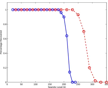
2.11 The probability of recovering a k-approximately-sparse signal with n= 1024 and m = 512 . . . 65

3.1 Allowable sparsity as a function of C (allowable imperfection of the recovered signal is 2(C_C+1)∆₋₁ ) . . . 72

3.2 The Grassmann angle for a skewed crosspolytope . . . 80

3.3 The combinatorial, internal and external angle exponents . . . 109

3.4 The combinatorial exponents and the angle exponents . . . 110

(14)

3.6 The weak, sectional and strong robustness bounds . . . 112 4.1 Illustration of a non-uniformly sparse signal . . . 132 4.2 A plot of asymptotes of external angle, internal angle and combinatorial

factor exponents for γ1 =γ2 = 0.5, P1 = 0.05, P2 = 0.3 and W_W2₁ = 1.5 . 138

4.3 δc as a function of W_W2₁ forP1 = 0.3 and P2 = 0.05 . . . 139

4.4 δc as a function of W_W2₁ forP1 = 0.65 and P2 = 0.1 . . . 139

4.5 Successful recovery percentage for weighted ℓ1 minimization with

differ-ent weights in a nonuniform sparse setting. P2 = 0.05 and m= 0.5n . . 161

4.6 Successful recovery percentage for different weights. P2 = 0.1 and m=

0.75n . . . 162 5.1 Recoverable sparsity factor forδ = 0.555, when the modified reweighted

ℓ1-minimization algorithm is used. . . 175

(15)

List of Tables

(16)

Chapter 1

Introduction

1.1

Motivations

Compressive sensing, also referred to ascompressed sensing orcompressive sampling, is an emerging area in signal processing and information theory which has attracted a lot of attention recently [CT06] [Don06b]. The motivation behind compressive sensing is to do “sampling” and “compression” at the same time. In conventional wisdom, in order to fully recover a signal, one has to sample the signal at a sampling rate equal or greater to theNyquist sampling rate. However, in many applications such as imaging, sensor networks, astronomy, high-speed analog-to-digital compression and biological systems, the signals we are interested in are often “sparse” over a certain basis. For example, an image of a million pixels has a million degrees of freedom, however, a typical interesting image is very sparse or compressible over the wavelet basis, namely, very likely only a small fraction of wavelet coefficients, say, one hundred thousand out of a million wavelet coefficients, are significant in recovering the original images, while the rest of wavelet coefficients are “thrown away” in many compression algorithms. This process of “sampling at full rate” and then “throwing away in compression” can prove to be wasteful of sensing and sampling resources, especially in application scenarios where such resources as sensors, energy, and observation time etc. are limited.

(17)

the high-dimensional signals exactly or accurately, by using a much smaller number ofnon-adaptive linear samplings or measurements. In general, signals in this context are represented by vectors from linear spaces, many of which in the applications will represent images or other objects. The fundamental theorem of linear algebra, “as many equations as unknowns,” tells us that it is not possible to reconstruct a unique signal from an incomplete set of linear measurements. However, as we said before, many signals such as real-world images or audio signals are often sparse or compress-ible over some basis, such as smooth signals or signals whose variations are bounded. This opens the room for recovering these signals accurately or even exactly from in-complete linear measurements. However, even though we know that the signal itself is sparse, it is a non-trivial job to recover the signals from the compressed measure-ments since we do not know the locations of the non-zero or significant components of that vector. One of the cornerstone techniques enabling compressive sensing is then about efficient and effective decoding algorithms to recover the sparse signals from the “compressed” measurements. One of the most important and popular decoding algorithms for compressive sensing is the Basis Pursuit algorithm [Che95, CDS98], namely the ℓ1-minimization algorithm.

1.2

Mathematical Formulation for Sparse

Recov-ery

Before we go into greater technical details in later chapters, we will first give the general signal models discussed in this thesis. We say that a n-dimensional signal x

is k-sparse if it has k or fewer non-zero components:

x_{∈ R}n, _kx_k0 :=|supp(x)| ≤k≪n,

where_|supp(x)_|denotes the cardinality of the support set ofx, and thus_k·k0, namely

(18)

k · kp the usual p-norm,

kx_k_p :=

n

X

i=1

|xi|p

1/p

,

and kx_k_∞ = max|xi|, where xi denotes the i-th component of the vector x. In the

case when signals are not exactly sparse, but their coefficients decay rapidly, we call these signals approximately sparse signals. In particular, compressible signals are those satisfying a power law decay:

|x∗i| ≤Li−

1

q, (1.2.1)

where x∗ is a non-increasing rearrangement of x, L is some positive constant, and 0< q <1. Of course, sparse signals are special cases of compressible signals.

Compressive sensing only measures sparse signals from a small set of non-adaptive linear measurements. Each measurement is seen as an inner product between the signal x_{∈ R}n and a measurement vector ai ∈ Rn, where i = 1, . . . , m. If we collect

mmeasurements in this way, we may then consider them_×nmeasurement matrix A

whose rows are the vectors ai. We can then view the sparse recovery problem as the

recovery of the k-sparse signal x_{∈ R}n from its measurement vector y=Ax_{∈ R}m. One may wonder how to reconstruct the signals from this incomplete set of mea-surements. With the prior information of the sigal being sparse, one of the theoreti-cally simplest ways to recover such a vector from its measurementsy=Axis to solve the ℓ0-minimization problem

min

x∈Rnkxk0 subject to Ax=y. (1.2.2)

If x is k-sparse and the rank of A is larger than 2k, then the solution to (1.2.2) must be the signal x. Indeed, if the solution is z, then since xis a feasible solution,

z must be k-sparse as well. Since Az = y, y ₋x must be in the null-space of

(19)

theoretically. However, it is computationally NP-Hard in general [CT05]. Fortunately, in the framework of compressive sensing, there have been computationally efficient relaxation algorithms for this computationally NP-Hard problem.

1.2.1

ℓ

1

Minimization

One major approach, Basis Pursuit, relaxes the ℓ0-minimization problem to an ℓ1

minimization problem:

min

x_∈Rnkxk1 subject to Ax=y. (1.2.3)

Simply put, instead of trying to find the solution with the smallest ℓ0-norm,ℓ1

min-imization tries to find the solution with the minimum ℓ1 norm. Surprisingly, this

relaxation often recovers x exactly when x is sparse or accurately when x is an ap-proximately sparse signal or compressible signal. Please note that the measurement matrixAis given and fixed in advance, and does not depend on the signal, but as long as the signals are sufficiently sparse and the measurement matrix satisfies some con-ditions independent of the signals, the ℓ1 minimization will succeed [CT05, Don06c].

That is, even though ℓ1-norm is different from the quasi-norm ℓ0, the solution of ℓ1

often comes as the sparsest solution.

As mentioned in [CT08], this sparsity-promoting feature of ℓ1 minimization was

already observed in the 1960’s by Logan [Log65], where he proved probably the first

ℓ1-uncertainty principle. Suppose we have the observation over time

y(t) =f(t) +n(t), t_{∈ R}, (1.2.4)

where f(t) is bandlimited, namely

(20)

if we recover f by the following program

minky−fˆkL1(R) subject to fˆ∈B(Ω), (1.2.6)

then the recovery is exact provided that |T||Ω| ≤ π/2. This holds for whatever

f _∈B(Ω) and for whatever values of the noise. ℓ1 minimization also appeared early

in reflection seismology, where people tried to infer a sparse reflection function (in-dicating meaningful changes between subsurface layers) from bandlimited data. For example, Taylor, Banks and McCoy and others began proposing the application of

ℓ1 for deconvolving seismic traces [TBM79] and a refined idea better handling the

observation noise was introduced in [SS86]. In the meanwhile, some rigorous theo-retical results started appearing in the late 1980’s, when Donoho and Stark [DS89] and Donoho and Logan [DL92] extended Logan’s 1965 result and quantified the abil-ity to recover sparse reflectivabil-ity functions from bandlimited data. With the LASSO algorithm [Tib96] proposed as a method in statistics for sparse model selection, the application areas for ℓ1 minimization began to broaden. Basis Pursuit [CDS98] was

proposed in computational harmonic analysis for extracting a sparse signal represen-tation from highly overcomplete dictionaries, and a related technique known as total variation minimization was proposed in image processing [GGI+_02].

It then came as a breakthrough in [CT05, CT06] and [Don06c] that Basis Pur-suit method was shown to be able to recover sparse signals with a linear fraction of non-zero elements. Certainly this requires some conditions on the measurement ma-trix A stronger than the simple rank conditions mentioned above. For example, the restricted isometry property (RIP) conditions were given in [CT05, CT06] to guar-antee that ℓ1 minimization accurately recovers sparse or compressible signals. It is

(21)

1.2.2

Greedy Algorithms

Theℓ1-minimization approach provides uniform guarantees over all sparse signals and

also stability and robustness under measurement noises and approximately sparse sig-nals, but relies on optimization which has relatively high complexity, for example, lin-ear programming, the complexity of which grows cubic in the problem dimensionn. In many applications which involve very large dimension processing, these approaches are not optimally fast. The other main approaches use greedy algorithms such as Orthogonal Matching Pursuit [MZ93, TG], Stagewise Orthogonal Matching Pur-suit [DTDS07], Regularized Orthogonal Matching PurPur-suit [NV09], Iterative Thresh-olding [FR07, BD] and Compressive Sampling Matching Pursuit (CoSaMP) [NT08]. Most of these approaches calculate the support of the signal iteratively. With the sup-port S of the signal calculated, the signal x is reconstructed from its measurements

y=Axasx= (AS)†y, whereASdenotes the measurement matrixArestricted to the

columns indexed by S and †denotes the pseudoinverse. Greedy approaches are rela-tively fast compared with the Basis Pursuit algorithm, both in theory and practice, but most of them deliver smaller recoverable sparsity compared to ℓ1 minimization

and most of them often come without provable uniform guarantees and stability, with the exception of [NV09, NT08].

1.2.3

High Dimensional Geometry for Compressive Sensing

The idea of compressive sensing and ℓ1 minimization certainly did not come from

nowhere. The theoretical foundation for compressed sensing is high dimensional ge-ometry, which is deeply connected with the field of geometric functional analysis. For example, Kashin in the 1970’s studied how many and what linear measurements (as described before) need to be taken so that we can recover a vector with a precision ǫ

from the ℓ1 ball,

(22)

After we know the measurement matrixA, we know that all the solutionsxto the underdetermined system lies in an affine space parallel to the null space of A. Then Kashin’s problem clearly becomes a high dimensional geometrical problem, which is about how we should select this null space so that the affine space’s intersection with the ℓ1 ball has minimal radius. The answer to this question was given by

Kashin [Kas77] and later refined by Garnaev and Gluskin [GG]. Their existential results rely on randomly choosing the linear projections (or measurements) and are optimal in order of the number of measurements, which is within a multiplicative factor of what the ℓ1 minimization compressive sensing provides. However, their

results were mostly existential while compressive sensing comes with at least one practical algorithm, theℓ1 minimization algorithm, which is nearly optimal over many

classes of signals.

In addition, the deep probabilistic techniques from [Bou89, BT, BT87, BT91], especially the generic chaining technique developed in [Bou89, Tal96], which controls the suprema of random processes, were used as important technical tools in verify-ing that certain measurement matrix ensembles satisfy the conditions for recoververify-ing sparse signals [CT06].

1.3

Applications

(23)

1.3.1

Compressive Imaging

Naturally, one of the most prominent applications of compressive sensing is to acquire images efficiently. The images we are interested in are often sparse over some basis so that they fit just into the framework of compressive sensing. Today’s digital cameras capture images with one sensor for each pixel and acquire every pixel in an image before compressing that captured data and storing the compressed image. Due to the use of silicon, everyday digital cameras today can operate in the megapixel range. Consistent with the motivation for compressive sensing, a natural question asks why we need to acquire this many data, just to throw most of it away immediately.

In the newly developed compressive imaging, the sensors directly acquire random linear measurements of an image while avoiding using sensors for each pixel. Compres-sive sensing provides a guideline framework for implementing such an idea, including designing the measurement methods and the decoding algorithms. Researchers have worked on the construction of such systems, for example, in a prototype “single-pixel” compressive sampling camera [WLD+_{06]. This camera consists of a digital}

micromirror device (DMD), two lenses, a single photon detector and an analog-to-digital (A/D) converter. The first lens focuses the light onto the DMD. Each mirror on the DMD is for a pixel in the image, and can be tilted toward or away from the second lens. This operation is analogous to creating inner products with random vectors. This light is then collected by the lens and focused onto the photon detector where the measurement is computed. This optical computer computes the random linear measurements of the image in this way and passes those to a digital computer that reconstructs the image.

(24)

In medical imaging, in particular in magnetic resonance imaging (MRI) which sample Fourier coefficients of an image, compressive sensing finds another important application. MR images are implicitly sparse: some MR images such as angiograms are sparse in their actual pixel representation, whereas more complicated MR im-ages are sparse over some other basis, such as the wavelet Fourier basis. As we all know, MRI in general is very time costly, as the speed of data collection is limited by physical and physiological constraints. Thus it is very helpful to reduce the number of measurements collected without sacrificing quality of the MR image, or said in another way, increasing the recovered image quality with the same number of mea-surements. In fact, compressive MRI is a very active topic in compressive sensing and has attracted a large number of researchers in this field. Many compressive sensing algorithms have been specifically designed for MRI application [LDP07].

1.3.2

Radar Signal Processing

A traditional radar system transmits some kind of pulse form, and then uses a matched filter to correlate the signal received with that pulse. The receiver then uses a pulse compression system together with a high-rate analog-to-digital (A/D) converter for signal processing. This conventional approach is not only complicated and expensive, but also the resolution in traditional radar system is limited by the radar uncertainty principle. Compressive Radar Imaging discretizes the time-frequency plane into a grid and treats each possible target scene as a matrix. If the number of targets is small enough, then the occupations of the grids will be sparse, and compressive sensing techniques can be used to recover the target scene [HS07].

1.3.3

Biology

(25)

sample is expensive, the method was to group people and test the entire pool of blood samples for this group. Only if syphilis antigen was found in a pool of samples, further testings into the subgroups of that group would then take place.

A more modern example of compressive sensing idea in biology is for comparative DNA Microarray [VPMH, MBSR]. Microarrays (DNA, protein, etc.) are massively parallel affinity-based biosensors capable of detecting and quantifying a large number of different genomic particles simultaneously. Generally, DNA microarrays comprising tens of thousands of probe spots are being used to test a multitude of targets in a single experiment. In conventional microarrays, each spot contains a large number of copies of a single probe designed to capture a single target, and hence collects only a single data point. But in comparative DNA microarray experiments, only a fraction of the total number of genes represented by the reference sample and the test sample is differentially expressed. So we can use the compressive ideas to create the so-called compressed microarrays [VPMH], wherein each spot contains copies of several different probes and the total number of spots is potentially much smaller than the number of targets being tested.

Gene expression studies also provide examples of compressive sensing. For exam-ple, one would like to infer the gene expression level of thousands of genes from only a limited number of observations [Can06].

1.3.4

Error Correcting

(26)

field, while on the contrary, traditional coding theory usually assumes data values over the finite field. Indeed there are many practical applications for encoding over the continuous reals. In digital communications, for example, one wishes to protect results of onboard computations that are real-valued. These computations are performed by circuits that experience faults caused by effects of the outside world. This and many other examples are difficult real-world problems of error correction.

The error correction problem can be formulated as follows, from where we can also see the close relationship between coding theory and compressive sensing. Consider a m-dimensional input vector f _{∈ R}m, the “plaintext,” that we wish to transmit reliably to a remote receiver. We transmit the n-dimensional coded text, namely “ciphertext,” z=Bf where B is the n×m coding matrix, or thelinear code. In the case of no noise, it is clear that if the linear codeB has full rank, we can recover the input vectorf from the ciphertextz. But as is often the case in practice, we consider the setting where the ciphertext z has been corrupted by sparse noises (similar to the finite field coding literature, a few bit errors). We then wish to reconstruct the input signalf from the corrupted received codewordz′ ₌_Bf₊_e_where_ε_{∈ R}n _{is the}

sparse error vector. To realize this in the usual compressed sensing setting, consider a matrixA whose null-space is the range ofB. ApplyAto both sides of the equation

z′ =Bf +ε to get Az′ =Aε. Set y =Bz′ and the problem becomes reconstructing the sparse vector εfrom its linear measurementsy. Once we have recovered the error vectorε, we have access to the actual measurements Af and, since Ais full rank, can recover the input signal f. For the details, please refer to [RIC, CT05].

1.4

Some Important Issues

(27)

1.4.1

Explicit Constructions of Sensing Matrices

There are several classes of random matrices used nowadays in compressive sensing, for example, random Gaussian matrices, random Bernoulli matrices, or random mi-nors of a discrete Fourier transform matrix, but they are all probabilistic in nature; in particular, these randomly constructed matrices are not perfectly guaranteed to actually produce a “good” sensing matrix, although in many cases the failure rate can be proven to be exponentially small in the size of the matrix. Moreover, there were no fast algorithms known to test whether any given matrix is a good measure-ment matrix, for example, satisfying the RIP condition [Tao07]. It is thus interesting to find a deterministic construction which can give and test “good” sensing matri-ces efficiently. In analogy with error-correcting codes, it may be that algebraic or number-theoretic constructions may give such deterministic “good” matrices; some efforts have been made towards this end, for example, in [DeV07] where determinis-tic sensing matrices with suboptimal sparsity parameters have been given. However, deterministic explicit efficient constructions of sensing matrices, which offers stable recovery of sparse signals with sparsity scaling linearly with the problem dimension, were elusive.

1.4.2

Efficient Decoding Algorithms with Provable

Perfor-mance Guarantees

In the compressed sensing literature, there have been many numerically feasible de-coding algorithms to the sparse recovery problem from compressed observations. One major approach, Basis Pursuit, relaxes the ℓ0-minimization problem to an ℓ1

-minimization problem. The ℓ1-minimization approach provides uniform guarantees

and stability, but relies on optimization methods for ℓ1-minimization, for example,

(28)

Match-ing Pursuit [NV09], and Compressive SamplMatch-ing MatchMatch-ing Pursuit (CoSaMP) [NT08]. These algorithms can provide similar uniform guarantees and stability results as the Basis Pursuit algorithm, but the complexity of these algorithms are growing super-linearly in the problem dimension. It would be interesting to design sensing matrices and decoding algorithms which are able to provide provable strong sparsity recov-ery performances while having low computational complexity, hopefully linear in the problem dimension.

1.4.3

Performance Analysis of Sparse Signal Recoveries

There are many algorithms for sparse signals recoveries, for example, theℓ1-minimization

algorithm. It is very important to understand how well these algorithms perform in recovering sparse signal recoveries, which is often characterized by the recoverable sparsity threshold. Thus what is in particular interesting then is to characterize the recoverable sparsity thresholds or sharp performance bounds for different decoding algorithms and measurement matrices. When the measured signals are not exactly sparse and the measurement results are corrupted by noises, we are more interested in analyzing the stability and robustness of these sparse signal recovery algorithms and how they interact with the signal sparsity. The analysis made for sparse signal recovery is often tightly connected to fundamental probabilistic or geometric phe-nomena and problems in high dimensional geometry, thus often advancing the fruit-ful interactions between signal processing, optimization theory and high dimensional geometrical and probabilistic analysis.

1.4.4

More than Sparse Vectors

(29)

and information tables). Some results have been obtained in this direction [RFP, CR09, RXH08a]. All the important technical challenges with compressive sensing also appear in these more general problems.

1.5

Contributions

The contributions of this thesis are closely related to addressing the problems of how to design these linear measurements, how to construct the original high-dimensional signals efficiently and accurately, and how to analyze the sparse signal recovery algo-rithms.

1.5.1

Expander Graphs for Explicit Sensing Matrices

Con-structions

As we mentioned before, explicitly constructible measurement matrices providing per-formance guarantees and linearly scaling sparsity recoverability were elusive and the

ℓ1 minimization methods are very demanding in computational complexity for

prob-lems with very large dimension. In chapter 2, we proposed and discussed a compres-sive sensing scheme with deterministic performance guarantees using deterministic explicitly constructible expander-graphs-based measurement matrices. Moreover, we showed that sparse signal recoveries can be achieved with linear complexity. This is the first of such a kind of compressive sensing scheme with linear decoding complex-ity, deterministic performance guarantees and deterministic explicitly constructible measurement matrices.

1.5.2

Grassmann Angle Analytical Framework for Subspaces

Balancedness

ℓ1 minimization algorithms generally give better sparsity recovery performances than

(30)

a necessary and sufficient null-space condition for achieving a certain signal recovery accuracy, we reduce the analysis of sparse signal recovery robustness to investigating a linear subspace balancedness property. Using high-dimensional geometry, we give a unified null-space Grassmann angle-based analytical framework for analyzing the linear subspace property. This new framework gives sharp quantitative tradeoffs between the signal sparsity and the recovery accuracy of the ℓ1 optimization for

approximately sparse signals.

1.5.3

Weighted

ℓ

1

Minimization Algorithm

The conventional approach to compressed sensing assumes no prior information on the unknown signal and a plain ℓ1 minimization was used. In chapter 4, we consider

a particular model for the sparse signal that assigns a probability of being zero or nonzero to each entry of the unknown vector. The standard compressed sensing model is therefore a special case where these probabilities are all equal.

We proposed to use weighted ℓ1 minimization algorithm for signal recovery under

this model. Assuming that the Gaussian measurement matrix ensemble is used, using the null-space Grassmann angle-based analytical framework, we are able to characterize the optimal recoverable sparsity thresholds, the optimal weights or the smallest number of measurement using weighted ℓ1 minimization algorithms under

the prior information.

1.5.4

An Analysis for Iterative Reweighted

ℓ

1

Minimization

Algorithm

Even though iterative reweighted ℓ1 minimization algorithms or related algorithms

(31)

information was able to be obtained in the process of iterations and this information can be utilized in the weighted ℓ1 minimization to boost the sparse signal recovery.

In particular, we showed that for a nontrivial class of signals, the iterative reweighted

ℓ1 minimization can indeed deliver recoverable sparsity thresholds larger than the ℓ1

minimization. Again, our results are based on thenull-space Grassmann angle-based analytical framework and the Gaussian measurement matrix ensemble.

1.5.5

Null Space Conditions and Thresholds for Rank

Mini-mization

Evolving from compressive sensing problems, we turned our attention to recovering matrices of low rank from compressed linear measurements in chapter 6.

Minimizing the rank of a matrix subject to constraints is a challenging problem that arises in many applications in machine learning, control theory, and discrete geometry. This class of optimization problems, known as rank minimization, is NP-HARD, and for most practical problems there are no efficient algorithms that yield exact solutions. A popular heuristic replaces the rank function with the nuclear norm—equal to the sum of the singular values—of the decision variable and has been shown to provide the optimal low rank solution in a variety of scenarios.

(32)

Chapter 2

Expander Graphs for Compressive

Sensing

As discussed, compressive sensing is an emerging technology which can recover a sparse signal vector of dimensionn via a much smaller number of measurements than

n. However, on the encoding side, there were no explicit constructions of “good” measurement matrices which come with guaranteed performances under computa-tionally feasible and robust decoding methods [Tao07]. On the decoding side, the known decoding algorithms have relatively high recovery complexity, such as O(n3_),

or can only work efficiently when the signal is super sparse, sometimes without deter-ministic performance guarantees. In this chapter, we propose a compressive sensing scheme using measurement matrices constructed from expander graphs. It is the first of its kind that comes withexplicit measurement matrix constructions, deterministic decoding performance guarantees with the capability of recovering signals withlinear sparsity, where the number of non-zero elements k grows linearly with n, and, at the same time, with linear (O(n)) decoding complexity. When the number of nonzero elements k does not grow linearly with the dimension n, similar to the ℓ1

minimiza-tion using dense random matrices, this scheme can exactly recover anyk-sparse signal using onlyO(klog(n/k)) measurements.

(33)

noise. Simulation results are given to show the performance and complexity of the new method and we also compare our work with recent works on expander graph based compressive sensing schemes.

2.1

Introduction

Compressive sensing has recently received a great amount of attention in the applied mathematics and signal processing community. The theory of compressive sensing, as developed over the past few years, attempts to perform sampling and compression simultaneously, thus significantly reducing the sampling rate. What allows this theory is the fact that, in many applications, signals of interest have a “sparse” representation over an appropriate basis. In fact, compressive sampling is intimately related to solving underdetermined systems of linear equations with sparseness constraints. The work of Cand`es, Romberg and Tao [CRT06, CT06] and Donoho [Don06c] came as a major breakthrough in that they rigorously demonstrated, for the first time, that, under some very reasonable assumptions, the solution could be found using simple linear programming—thus rendering the solution practically feasible. The method is essentially constrained ℓ1 minimization, which for a long time was empirically known

to perform well for finding sparse solutions and has been known in the literature as “Basis Bursuit” [Che95, CDS98]. Interestingly, the area of compressive sensing is closely connected to the related areas of coding [CT05], high-dimensional geometry [DT05a], sparse approximation theory [Don06a], data streaming algorithms [CM06, GSTV05] and random sampling [GGI+_{02]. Furthermore, promising applications of}

compressive sensing are emerging in compressive imaging, medical imaging, sensor networks and analog-to-digital conversion [Can06].

While solving the linear program resulting from ℓ1 optimization can be done in

polynomial-time (oftenO(n3_{), where}_n _{is the number of unknowns), this may still be}

infeasible in applications where n is quite large (e.g., in current digital cameras the number of pixels is of the order n= 106 _{or more) [CR]. Therefore there is a need for}

(34)

the previous works, random measurement matrices are used where a successful signal recovery can not be always guaranteed although it succeeds with a high probability. So it is also desirable to have an explicit construction of a measurement matrix for compressive sensing [Can06, DeV07].

2.1.1

Related Works

Recently, some significant progress has been made in addressing these two problems for compressive sensing. Orthogonal Matching Pursuit (OMP) algorithms can be used as alternative recovery algrithms which require O(nk2_{) computations [TG], where} _k

is the number of non-zero entries in the unknown vector; however, this may also be too high a complexity. Stage-wise OMP [DTDS07] has recently been proposed that solves the problem in O(nlogn) computations. In [CM06] a certain sparse coeffi-cient matrix has been used, along with group testing, that yields an algorithm with

O(klog2n) complexity; however, this comes at the expense of more measurements—

O(klog2n) measurements, as opposed to theO(klogn) measurements required of the aforementioned methods. Chaining pursuit has been introduced in [GSTV05], which has complexity O(klog2nlog2k) and also requires O(klog2n) measurements. From the number of measurements needed, we can see that both the group testing methods [CM06] and the chaining pursuit methods only work in the “supersparse” case, i.e., when the ratio k/n is very small—when k/n is increased, an enormous number of measurements is required, as noted in [SBB06a]. Motivated by low-density parity-check codes (LDPCs) a method called sudocodes has been proposed in [SBB06b] to recover sparse signal with high probability, which requires O(klognlogk) recovery complexity, yet only O(klogn) measurements. The Homotopy methods are able to recover the sparse solutions by reducing the computational complexity from O(n3₎

to O(nk2_{) [DT06a]. In [Fuc04], it was shown that by using the Vandermonde}

(35)

in [SBB06b], a scheme of recovery complexityO(k2_{) is proposed to recover any signal}

vector with k nonzero elements using the Vandermonde measurement matrix. List decoding was proposed for similar schemes in [PH08].

With the exception of the method in [DeV07], the group testing methods in [CM06] and the Vandermonde measurement matrix-based methods in [Fuc04, AT07], all the results described above hold with “high probability” either over the random mea-surement matrix or over some assumptions on the input signals [SBB06b]. While the methods in [DeV07, CM06] can guarantee sparse signal recovery deterministically with explicit measurement matrices, they suffer from the fact that they only work in the supersparse case where k can not be kept as a constant fraction of n. But recov-ering a constant fraction of nnon-zero elements via a small number of measurements is of great practical interests [CT05]. For this reason, in this chapter, we will allow

k to grow linearly in n, i.e., k = Θ(n). In this sparsity regime, the complexity of the methods of [Fuc04, AT07] are of order O(n3_{) and} _O₍_n2_{) respectively, which will}

still be impractical for problems of large dimensions. Sometimes, it is also required that the recovery schemes are applicable to approximately sparse signals and robust to the noise in the measurements and numerical errors.

2.1.2

Contributions

In this chapter, we propose a new scheme for compressive sensing with deterministic performance guarantees based on bipartite expander graphs and show that even with

(36)

which are related to expander graphs [SS96], but in our works we provide performance guarantees. Preliminary analytic results further show the feasibility of application of the new method to approximately sparse signals and the noisy measurement cases. When the number of nonzero elementsk does not grow linearly with the dimensionn, similar to the ℓ1 minimization using dense random matrices, this scheme can exactly

recover any k-sparse signal using only O(klog(n/k)) measurements.

2.1.3

Recent Developments

After the publication of our works [XH07a, XH07b], an explicit construction for com-pressive sensing matrices was given in [Ind08] which used extractors. But the con-struction in [Ind08] only works for recovering sparse signals with sublinear sparsity. In a more recent very interesting work [BGI+_{08], it was shown that the expander}

graph-based measurement matrices can work with performance guarantees under the

ℓ1 minimization methods. Indyk and Ruzic [IR08], and Berinde, Indyk and Ruzic

[BIR08] proposed new compressed sensing algorithms based on the properties of the expander graphs. Those algorithms are similar to the CoSaMP algorithm [NT08], from the orthogonal matching framework, and are designed to be robust against more general noise and compressible signals; however, this comes with a cost on com-plexity of the algorithm and its analysis. The algorithm that we proposed in this chapter is much simpler, and also the analysis on why the algorithm works is only based on the unique neighborhood properties of the expander graphs. In contrast, the other algorithms require expander graphs with stronger expansion and a complicated preprocessing step, and the analysis is based on more involved properties of expander graphs with larger expansions.

The rest of this chapter is organized as follows. In the next section we review the background and give the problem formulation. We introduce expander graphs in Section 2.3 and show how they can be used to develop deterministic methods with

(37)

property are described in Section 2.6. Optimized expander graphs are used in Section 2.7 to reduce the number of iterations to O(k). Simulation results are given in the section 2.8.

2.2

Background and Problem Formulation

In compressive sensing the starting point is an n-dimensional signal vector which admits a sparse representation in some particular basis. Since the basis is not of primary concern to us, we may, without loss of generality, assume that it is the standard basis. In other words, we shall assume that we have an n-dimensional vector x_{∈ R}n_{, such that no more than} _k _{entries are non-zero. Clearly,} _{k < n}_{. Here}

we assumek can be up to a constant fraction ofn, since this case is of great practical interest [CT05].

The vectorxitself is not directly observable. What is observable aremeasurements of x that correspond to linear combinations of the form

n

X

j=1

ajxj. (2.2.1)

We often have control over what measurements to employ, and this may turn out to help us. In any event, assuming we have m (k < m < n) measurements of this form, we may collect them in a m_×n matrix A so that

y=Ax, (2.2.2)

or, in other words,

yi = n

X

j=1

Aijxj, i= 1, . . . , m. (2.2.3)

(38)

CT06] and Donoho [Don06c] that, under the sparsity assumption, the solution could be found via solving the ℓ1 optimization problem

min

x,Ax=ykxk1, (2.2.4)

where _kx_k1 =Pn_i₌₁|xi| is theℓ1-norm of the vector x. The upshot is that something

that appeared to be practically infeasible can now be potentially computed. For example, in [CT05], it was shown that if the measurement matrix A satisfies the restricted isometry conditions, then theℓ1 minimization can recover a vector with up

tok nonzero elements, where k is a constant fraction of n.

In spite of the recent developments, one unanswered question is whether we can develop compressive sensing schemes and recovery algorithms with complexity O(n) even whenk = Θ(n)? If yes, can oneexplicitly develop constructions of measurement matrices that deterministically guarantee finding the optimal solution for all signal instances in such schemes, provided the vector xis sparse enough? We shall presently answer both questions in the affirmative and discuss all these developments in the next section.

2.3

Expander Graphs and Efficient Algorithms

2.3.1

Expander Graphs

(39)

In particular,

Aij =

 



1 if right node i connected to left nodej

0 otherwise

(2.3.1)

for i = 1, . . . , m and j = 1, . . . , n. In what follows we shall use the matrix thus obtained from a suitably chosen bipartite graph as the measurement matrix for com-pressive sampling.

...

1 2 3

n

1 2

[image:39.612.267.384.247.337.2]

m

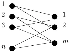
Figure 2.1: A bipartite graph

A bipartite graph will be said to have regular left degree cif the number of edges emanating from each variable node is c.

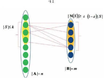
Definition 2.3.1 (Expander). A bipartite graph with n variable nodes, m parity check nodes and regular left degree c will be called a (αn, βc) expander, for some 0 < α, β < 1, if for every subset of variable nodes V with cardinality less than or equal to αn, i.e., _{|V| ≤} αn, the number of neighbors connected to _V is larger than

βc|V|, i.e., |N(V)|> βc|V|, where N(V) is the set of neighbors of V.

Here we assume that each righthand side node also has a regular degree d, where

(40)

[CRVW02]. An existence result, which holds for the setting we are interested in, is the following [BM01]:

Theorem 2.3.2. Let 0< β <1and the ratio r= m_n be given. Then for large enough

n there exists a regular left degree c and a regular right degree d bipartite expander (αn, βc) for some 0< α <1 and some constant (not growing with n) c.

2.3.2

The Main Algorithm

We are now in a position to describe our main algorithm. We begin with β = 3 4 and

some fixed r = m_n. (Thus, our number of measurements is m =nr. We can use the construction of [CRVW02], or any other recent one, to construct an expander with some 0< α <1 and constant c.) Denote the resulting measurement matrix by A. In particular, assuming x_{∈ R}n _{is sparse with at most}_k _{nonzero entries, we perform the}

m measurements

y=Ax. (2.3.2)

We will assume that

k ≤ αn

2 . (2.3.3)

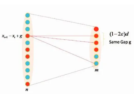
We need one further notation: given an estimate ˆx of x, we define as the gap in the i-th equation the quantity

gi =yi− n

X

j=1

Aijxˆj. (2.3.4)

Algorithm 1 is incredibly simple. What is remarkable about it is that, in step 2 of the algorithm, if y6=Axˆ one can always find a variable node with the property that

c′ _> c

2 among the measurement equations it participates in have identical nonzero

gap g. Furthermore, the algorithm terminates in at most ck steps. We proceed to establish these two claims via a series of lemmas. At any step of the algorithm, let _S denote the set

(41)

Algorithm 1

1: Start with ˆx= 0n×1.

2: if y =Axˆ then

3: declare ˆx the solution and exit. 4: else

5: find a variable node, say ˆxj, such that of the c measurement equations it

par-ticipates in c′ _> c

2 of them have an identical nonzerogap g.

6: Set ˆxj = ˆxj+g. Go to 2.

7: end if

Lemma 2.3.3 (Initialization). When xˆ= 0 ,y₆=Axˆ and k _≤ αn

2 , there always exists

a variable node such that c′ _> c

2 of the measurement equations it participates in has

identical nonzero gap g.

Proof: Initially since ˆxi = 0, the set S has cardinality |S| = k ≤ αn/2. We can

therefore apply the property of the expander with β = 3₄ to _S to conclude that

|N(_S)_|> 3

4c|S|. (2.3.6)

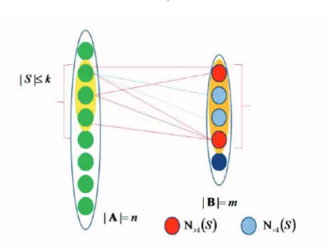
Let us now divide the set N(S) into two disjoint sets: Nunique(S) comprised of those

elements of_N(_S) that are connected to only one edge emanating from_S and_N>1(S)

which are the remaining elements ofN(S) that are connected to more than one edges emanating from_S. Clearly, (2.3.6) implies

|Nunique(S)|+|N>1(S)|>

3

4c|S|. (2.3.7)

Counting the edges emanating from _S leads to

|Nunique(S)|+ 2|N>1(S)| ≤c|S|, (2.3.8)

since the total number of edges is c|S| and since some of the nodes in N>1(S) may

have more than 2 edges connecting to _S. Eliminating _|N>1(S)| from the inequalities

(2.3.7) and (2.3.8) yields

|Nunique(S)|>

c

(42)

The above inequality implies that there must be at least one element of S that is connected to c′ _> c

2 elements of Nunique(S). But since this is the only element of

S connected to these c′ _{measurements, and since the} _A

ij’s are all 1 for the edges

connecting these nodes, they must all have the same nonzero gap g.

We now need another definition. At any step of the algorithm, let _T denote the set

T =

(

i_|yi 6= n

X

j=1

Aijxj

)

. (2.3.10)

Lemma 2.3.4 (Decrease in|T |). After the first step of the algorithm, the cardinality of the set _T decreases at least by 1.

Proof: According to the proof of Lemma 2.3.3, we have found a variable node with

c′ _> c

2 measurements with identical nonzero gap g. Setting ˆxj = ˆxj+g sets the gap

on thesec′ _{equations to zero. However, it may make some zero gaps on the remaining}

c₋c′ _{measurements nonzero. Nonetheless, since}_c′₋₍_c₋_c′_{) = 2}_c′₋_c_≥_{1 (note that}

c′₋_c/₂_≥ 1

2) the cardinality ofT decreases at least by one.

We can now proceed to the main induction argument.

Lemma 2.3.5 (Induction). Consider a regular left degree c bipartite graph with n

variable nodes and mparity check nodes. Assume further that the graph is an(αn,3 4c)

expander and consider Algorithm 1. If for all iterations of the algorithm up to step l: (1) S(l′)< αn, l′ = 1, . . . , l, where S(l′) is the same definition as in (2.3.5), except

for at the l′_{-th iteration.}

(2) There always exists a variable node such that c′ _> c

2 of the measurement

equa-tions it participates in have identical nonzero gap g.

(3) T(l′) ≤ T(l′−1) −1, for l′ = 1, . . . , l , where T(l′) is the same as in the

definition (2.3.10), except at the l′_{-th iteration.}

(43)

(i) S(l+1)< αn

(ii) If y 6=Axˆ, there always exists a variable node such that c′ _> c

2 of the

measure-ment equations it participates in have identical nonzero gap g. (iii) T(l+1)≤T(l)−1

Proof: Let us begin with claim (ii). The argument is very similar to that of the proof of Lemma 2.3.3, which we essentially repeat here. Due to assumption (1) in the lemma, S(l) < αn. Therefore we can apply the property of the expander with β = 3

4 to S

(l) _{to conclude that}

N(S(l))> 3

4c

S(l). (2.3.11)

As before, we divide the set _N(_S(l)_{) into two disjoint sets:} _N

unique(S(l)) comprised of

those elements of N(S(l)_{) that are connected to only one edge of} _S(l) _and _N

>1(S(l))

which are the remaining elements of _N(_S(l)_{) that are connected to more than one}

edges emanating fromS(l)_{. Clearly, (2.3.11) implies}

N_unique(S(l))+N_>₁(S(l))> 3

4c

S(l). (2.3.12)

Counting the edges emanating from _N(S(l)_{) leads to}

N_unique(S(l))+ 2N_>₁(S(l))≤cS(l), (2.3.13)

since the total number of edges is cS(l) and since some of the nodes in N_>₁(S(l))

may have more than 2 nodes emanating from them. EliminatingN_>₁(S(l))from the

inequalities (2.3.12) and (2.3.13) yields

N_unique(S(l))> c

2

S(l), (2.3.14)

which implies that there must be at least one element of _S(l) _{that is connected to}

c′ _> c

(44)

to these c′ _{nodes, and since the} _A

ij’s are all 1 for the edges connecting these nodes,

they must all have the same nonzero gap g.

This establishes (ii). Establishing (iii) is similar to the proof of Lemma 2.3.4. We have already found a variable node withc′ _> c

2 measurements with identical nonzero

gap g. Setting ˆx(_jl+1) = ˆx_j(l)+g sets the gap on thesec′ _{equations to zero. However, it}

may make some zero gaps on the remainingc₋c′ _{measurements nonzero. Nonetheless,}

since c′ ₋₍_c₋_c′_{) = 2}_c′₋_c _≥ _{1 (note that} _c′ ₋_c/₂ _≥ 1

2), the cardinality of T(l+1)

decreases at least by one compared to _T(l)_.

This establishes (iii). We finally turn to (i). Note that, since in each iteration of Algorithm 1 we change the value of only one entry of ˆx, the cardinality of the set

S(l′₎

can change at most by one. Since, due to assumption (1) of the lemma we have

S(l) _{< αn}_{, (iii) can only be violated if}_S(l+1) ₌_αn_{. Let us assume this and arrive at}

a contradiction. Note that we can apply the property of the expander with β = 3₄ to the set _S(l+1) _{to obtain}

N(S(l+1))> 3

4cαn. (2.3.15)

Once again, we divide the set N(S(l+1)_{) into two disjoint sets:} _N

unique(S(l+1)) and

N>1(S(l+1)). Clearly, (2.3.15) implies

N_unique(S(l+1))+N_>₁(S(l+1))> 3

4cαn. (2.3.16)

Counting the edges emanating from _N(S(l+1)_{) leads to}

N_unique(S(l+1))+ 2N_>₁(S(l+1))≤cαn (2.3.17)

since the total number of edges is cαn and since some of the nodes in_N>1(S(l)) may

have more than 2 nodes emanating from them. (2.3.16) and (2.3.17) imply

N_unique(S(l+1))> c

2αn. (2.3.18)

(45)

conclude that Nunique(S(l+1))⊆ T(l+1). This in turn implies that

T(l+1)> c

2αn. (2.3.19)

Note, however, that since k ≤ αn/2 and the left degree of the graph is c, at the beginning of the algorithm we haveT(0)≤ c

2αn. However, from assumption (3) and

property (iii), which we just established, we know thatT(l′)_{is a decreasing function}

for all l′ _≤_l_{+ 1. Therefore,}

T(l+1)<T(0)≤ c

2αn, (2.3.20)

which contradicts (2.3.19). This establishes (i) and hence all claims of the lemma. The above sequence of lemmas establishes the following main result regarding Algorithm 1.

Theorem 2.3.6 (Validity of Algorithm 1). Consider a regular left degree bipartite graph with n variable nodes and m parity check nodes. Assume further that the graph is an (αn,3₄c) expander and consider its corresponding A matrix. Let x ∈ Rn

be an arbitrary vector with at most k _≤ αn/2 nonzero entries and consider the m

measurements

y=Ax. (2.3.21)

Then Algorithm 1 finds the value of x in at most kc_≤ c

2αn iterations. If we assume

that the bipartite graph has a regular right degree, we will have a recovery algorithm with complexity linear in n.

Proof: The theorem has essentially been proven in Lemmas 2.3.3, 2.3.4 and 2.3.5. We essentially have shown that at each iteration the cardinality of the set _T(l) _decreases

by at least one. Since the initial cardinality is at mostkc,T(l) _{will be empty after}_at

most kc steps. But, of course, an empty _T(l) _{implies that the algorithm has found} _x

(46)

essentially the same arguments as in the proof of Lemma 3). If the bipartite graph has a regular right degree, then in each iterative step of algorithm 1, we only need a fixed number of operations to update the variable nodes and its related measurements by keeping track of the list of variable nodes.

Remarks

Here we can allow fork = Θ(n) nonzero entries inxsinceαis a constant (not going to zero asngrows) which depends on the expander graph. The number of measurements is m=rn, where r can take any value from (0,1) and determines the value of α.

2.4

Expander Graphs for Approximately Sparse

Signals

In this section, we will give preliminary analytic results on expander graph-based compressive sensing for approximately sparse signals. In an approximately sparse signal vector, only a few signal entries are significant and the remaining signal entries are near zero but possibly not exactly zero. In practice, the approximately sparse model is a more realistic model for signals. Here we use the same measurement matrix as in the previous section except that we apply it to approximately sparse signals. We also assume a two-level (“near-zero” and “significant”) signal model for the approximately sparse signal vector. (Of course, this is a coarse signal model, but it captures the nature of approximately sparse signal vectors.) The entries of the “near-zero” level in the signal vector are near-zero elements taking values from the set [₋λ,+λ] while the “significant” level of entries take values from the set_{x_|(L₋∆) _≤

|x| ≤(L+ ∆)}, where L >∆ andL > λ. Let ρ=max{2∆, λ} and d be the regular right check node degree. Now we apply the following signal recovery algorithm to y

with the measurement matrix A.

The following theorem establishes the validity of Algorithm 2.

(47)

Algorithm 2

1. Start with ˆx= 0n×1.

2. If _ky ₋ Axˆ_k_∞ _≤ ρd, determine the positions and signs of the significant components in xas the positions and signs of the non-zero signal components in ˆx; exit.

Else, find one variable node, say ˆxj, such that of thecmeasurement equations

it participates in c′ _> c

2 of them are in either of the following categories:

(a) They have gaps which are of the same sign and have absolute values betweenL₋∆₋λ₋ρ(d₋1) andL+ ∆ +λ+ρ(d₋1). Moreover, there exists a number t in the set {x|x = 0,|x| = (L−∆),|x| = (L+ ∆)}

such that _|y₋Axˆ_| are all_≤ρd over thesec′ _{measurements if we change}

ˆ

xj tot.

(b) They have gaps which are of the same sign and have absolute values between 2L₋2∆₋ρ(d₋1) and 2L+ 2∆ +ρ(d₋1). Moreover, there exist a number tin the set {x|x= 0,|x|= (L−∆),|x|= (L+ ∆)}such that _|y₋Axˆ_| are all _≤ρd over these c′ _{measurements if we change ˆ}_x

j

to t.

3. Reset ˆxj =t. Go to 2.

nodes and m parity check nodes. Assume further that the graph is an (αn,3 4c)

ex-pander with regular right degree d and regular left degree c. Denote the corresponding measurement matrix as A. Let x_{∈ R}n _{be an arbitrary vector with at most} _k _≤_αn/₂

significant signal components and assume that max_{ρ(2d₋1) + ∆ +λ, ρ(2d₋2) + 3∆ +λ}< L. Consider the m measurements

y=Ax. (2.4.1)

Then Algorithm 2 correctly finds the sign and positions of the significant components of x in at most kc≤ c

2αn iterations with complexity linear in n.

Proof: The arguments here basically follow the same reasoning as in the proof of Lemma 2.3.3, Lemma 2.3.4, Lemma 2.3.5 and Theorem 2.3.6. But now we define the set _S as the set of variable nodesj’s such thatxj and ˆxj are on different signal levels

(48)

nodej ∈S, thenL−∆−λ≤ |xj−xˆj| ≤L+∆+λor 2(L−∆)≤ |xj−xˆj| ≤2(L+∆).

Also notice that _|xj −xˆj| ≤ ρ if xj and ˆxj are both in the near-zero signal level or

have the same sign while both being on the “significant” signal level. Define the set

T as the set of measurements where _|y₋Axˆ_| have values larger thanρd. Notice that after each iteration, we can always decrease the cardinality of T by at least 1.

Now let us consider the case where the measurements themselves are not perfect and corrupted by additive noises. In this case, we have

y =Ax+w, (2.4.2)

wherewis am-dimensional noise vector. We assume|w|∞≤εand thatxis generated

according to the same approximately sparse signal model as stated previously. Then the previous algorithm and can be extended to the noisy measurements cases.

Algorithm 3

1. Start with ˆx= 0n×1.

2. If ky−Axˆk∞ ≤ ρd+ε, determine the positions and signs of the significant

components in xas the positions and signs of the non-zero signal components in ˆx; exit.

Else, find one variable node, say ˆxj, such that of thecmeasurement equations

it participates in c′ _> c

2 of them are in either of the following categories:

(a) They have gaps which are of the same sign and have absolute values betweenL−∆−λ−ρ(d−1)−εandL+ ∆ +λ+ρ(d−1) +ε. Moreover, there exists a numbertin the set_{x_|x= 0,_|x_|= (L₋∆),_|x_|= (L+∆)_} such that _|y₋Axˆ_|