The DCA:SOMe comparison: a comparative study between two biologically inspired algorithms

1 2 3 4 5 6 7 8 9 10 11 12 13 14 15 16 17 18 19 20 21 22 23 24 25 26 27 28 29 30 31 32 33 34 35 36 37 38 39 40 41 42 43 44 45 46 47 48 49 50 51 52 53 54 55 56 57 58 59

Evolutionary Intelligence manuscript No. (will be inserted by the editor)

Julie Greensmith · Jan Feyereisl · Uwe Aickelin

The DCA: SOMe Comparison

A comparative study between two biologically-inspired algorithms

Received: date / Accepted: date

Abstract The Dendritic Cell Algorithm (DCA) is an immune-inspired algorithm, developed for the purpose of anomaly detection. The algorithm performs multi-sensor data fusion and correlation which results in a ‘context aware’ detection system. Previous applications of the DCA have included the detection of potentially malicious port scanning activity, where it has produced high rates of true positives and low rates of false positives. In this work we aim to compare the performance of the DCA and of a Self-Organizing Map (SOM) when applied to the detection of SYN port scans, through experimental analysis. A SOM is an ideal candidate for comparison as it shares similarities with the DCA in terms of the data fusion method employed. It is shown that the results of the two systems are comparable, and both produce false positives for the same processes. This shows that the DCA can produce anomaly detection results to the same standard as an established technique.

Keywords Dendritic Cell Algorithm·Self-Organizing Map ·SYN scan detection·comparison

1 Introduction

The Dendritic Cell Algorithm (DCA) is an immune-inspired algorithm, which is the latest addition to a family of algorithms termed Artificial Immune Systems (AIS). Such systems use abstract models of particular components of the human immune system to produce systems which perform similar computational tasks to those seen in the human body. Previous approaches drew inspiration from the adaptive immune system producing algorithms such as clonal selection [14] and negative selection [33]. The negative selection approach has been used extensively in the domain of computer security specif-ically in the detection of potential intrusions [44]. Such systems enjoyed initial success, but have since been plagued with problems regarding scalability and the generation of excessive numbers of false positive alerts.

Aickelinet al.[1] proposed an alternative which suggests that successful AIS should be constructed using the ‘danger theory’ as inspiration. The danger theory suggests that the immune system responds to signals generated by the host cells (i.e. by the tissue) during cell stress, ultimately leading to the targeting of proteins present under the conditions of cell stress. It is a competing immunological theory, though it is still widely debated within immunology itself. This theory is centred around the detection of ‘danger signals’, which are released as a result of unplanned cell death, a process termed necrosis. Upon the detection of danger signals, the immune system can be activated. In the absence of necrosis, cells may die in a controlled manner as part of the regulatory processes found within the tissue, in a Julie Greensmith, Jan Feyereisl and Uwe Aickelin

School of Computer Science University of Nottingham Wollaton Road

1 2 3 4 5 6 7 8 9 10 11 12 13 14 15 16 17 18 19 20 21 22 23 24 25 26 27 28 29 30 31 32 33 34 35 36 37 38 39 40 41 42 43 44 45 46 47 48 49 50 51 52 53 54 55 56 57 58 59

process calledapoptosis. Dendritic cells (DCs) are sensitive to both signal types and have the ability to stimulate or suppress the adaptive immune system. DCs are the intrusion detection agents of the human immune system, policing the tissue for potential sources of damage in the form of signals and for potential culprits responsible for the damage in the form of ‘antigen’. Antigens are proteins which can be ‘presented’ to the adaptive immune system by DCs, and can belong to pathogens or to the host itself.

The DCA incorporates danger-based DC biology to form an algorithm that is both truly bio-inspired and is capable of performing anomaly detection. It is a population based algorithm, where multiple DCs are programmed to process signals and antigen. ‘Signals’ are mapped to context information, such as the behaviour of a monitored, e.g. CPU usage or network traffic statistics. ‘Antigens’ are mapped as potential causes for the changes in behaviour, e.g. the system calls of a running program. The DCA correlates the antigen and signal information across the population of cells to produce a consensus coefficient value which is assessed to determine anomalous antigen.

The DCA has been successfully applied to a subset of intrusion detection problems, focussing on port scan detection. Port scans are used to establish network layout and to uncover vulnerable computers. The detection of the scanning phase of an attack can be highly beneficial, as upon its detection the level of security can be increased across a network in response. The DCA has been applied to both ping scans and SYN scans in realtime and offline [27] [25]. The algorithm produced high rates of true positives and low rates of false positives.

While the performance of the DCA on these problems appears to be good, thus far no direct comparison has been performed with another system on the same port scan data. The need for a rigorous comparison is necessary to truly demonstrate the capabilities of this algorithm. The signal processing component housed within the DCA bears some resemblance to the function of a neural network [13]. Given these superficial similarities, the obvious next-step for the development of the DCA is to compare its performance to that of a neural network based system, such as a Self-Organizing Map (SOM) [47].

SOM is a clustering method of unsupervised learning where high dimensional data is mapped to a lower dimensional space to create a feature map. This map is constructed from training data and consists of a series of interconnected nodes. Upon the analysis of the test data, the incoming data items are matched against nodes in the map with similar characteristics. SOM uses a similar process to a single-layer neural network to generate the map, and a simple distance metric is used to match the incoming test data to the most appropriate node. This technique can be used for anomaly detection as the training data can consist of normal data items, with unclustered data representing a potential anomaly. SOM is an excellent choice for comparison as it has a history of application within computer security and can be manipulated to use similar input data as used with the DCA.

The aim of this paper is to compare the DCA with a SOM. To achieve this aim the two algorithms are applied to the detection of an outbound SYN-based port scan using data captured from previous real-time experiments performed with the DCA [25]. The results of this comparison indicate that the DCA and SOM are both equally as effective at detecting SYN based port scans, and appear to make similar false positive errors. As a baseline a k-means clustering algorithm is applied to the signals in isolation.

This paper is structured as follows. In Section 2, the relevant background and context information is given regarding problems in computer security and how these problems relate to port scanning in addition to a summary of current port scanning techniques. In Sections 3 and 4, descriptions are given of the DCA and SOM respectively, including details of their implementations. In Section 5, the two approaches are compared experimentally. In Section 6 we perform an analysis and comparison between the two systems based on the obtained results and debate their differences and similarities, further validated by a baseline series. In the final sections we discuss the results of these comparisons and present the implications for the future of the DCA.

2 Related Work

2.1 Overview

1 2 3 4 5 6 7 8 9 10 11 12 13 14 15 16 17 18 19 20 21 22 23 24 25 26 27 28 29 30 31 32 33 34 35 36 37 38 39 40 41 42 43 44 45 46 47 48 49 50 51 52 53 54 55 56 57 58 59

scan detection techniques. This is followed by the related computer security work in AIS, including the development of the DCA and the motivation for its development. This section continues with a brief overview of the use of various SOM algorithms in computer security.

2.2 Port Scanning and Detection

2.2.1 Introduction to Port Scanning

Insider attacks are one of the most costly and dangerous attacks performed against computerised systems, with a large amount of known intrusions of intrusions attributed to internal attackers [6]. This type of intrusion is defined through the attacker being a legitimate user of a system who behaves in an unauthorised manner. Such insider attacks have the potential to cause major disruption given that a large number of networks do not employinternal firewallingwith many security countermeasures focussing on the detection of external intruders. Insiders frequently know and have access to network topology information. As insiders operate from within an organisation, this provides them with scope to abuse a weak link in the security chain, namely the end users. Having knowledge and relationships with other network users brings with it the potential to coerce passwords from legitimate users for the purpose of gaining access across multiple machines on a network. This information can be used to steal sensitive data, to cause damage to the network or to disguise the identity of the true attacker.

Such attacks frequently involve multiple stages. The initial stage is the information gathering stage, which is followed by monitoring of potential victims, finally involving an intrusion. The information gathering stage involves scouting the network for potential victim host machines to suit the nature of the attack. For example, the insider may wish to exploit an FTP service and would therefore search the network for hosts running FTP. Port scanning is used in the information gathering stage to retrieve which hosts are currently running on the network, the IP addresses and DNS names of each host, which ‘ports’ are currently ‘open’ and named running host services.

It is wise for an attacker to understand the network in question, to avoid wasting time trying to exploit machines which are not receptive to an attack. It is pointless attempting to attack a host which is no longer connected to the network! While scanners are not an ‘intrusion’ in the classical sense, they are often a pre-cursor to an actual attack, and evidence of sufficient scanning across a network can suggest that an attack may soon follow [39].

A port is a specific endpoint on a network, which is a virtual address as part of a virtual circuit. It is important to note that a port in this context is an abstract concept, not to be confused with a physical port such as a serial port. Ports allow for the direct exchange of information between two hosts. It is similar to a telephone number and is more specific than an IP address as it provides a direct connection between two endpoints. Probing a port with a packet leads to information on the state of the port and its host. Ports can be in three states if the scanned host is available, namely open, closed or filtered. Port scanning tools such asnmap[17] can be used to send packets to various ports on remote hosts to gain understanding regarding the status of the scanned host. The type of packet used to perform such probes can be one of a number of types, including Internet Control Message Protocol (ICMP) ping, TCP, and UDP. According to Bailey-Leeet al.[4], TCP SYN scans are the most commonly observed scan, accounting for over half of all scans performed.

Additionally the scans themselves can be performed in a number of different ways, varying the number of hosts scanned, the number of ports scanned, the IP address of the sender and the rate at which packets are sent. The combination of the number of hosts (IP addresses) scanned and the number of ports gives rise to three combinations of scan:

– Horizontal Scans: A wide range of IP addresses are scanned, though only one port per host is

probed. This kind of scan can be used if a particular service is to be exploited, such as an FTP exploit whose success would depend on finding a host running the particular version of an FTP server/client.

– Vertical Scans: A range of ports are specified for a single IP address. This is a scan of a single

1 2 3 4 5 6 7 8 9 10 11 12 13 14 15 16 17 18 19 20 21 22 23 24 25 26 27 28 29 30 31 32 33 34 35 36 37 38 39 40 41 42 43 44 45 46 47 48 49 50 51 52 53 54 55 56 57 58 59

Attacker

Victim host present with open ports

SYN

SYN/ACK

RST

Victim

Attacker

Victim host present with closed ports

SYN

RST

Victim

Attacker

Victim host not attached to IP address

Firewall SYN

RST

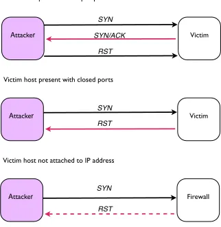
Fig. 1 The TCP/IP packet flow for SYN scans under various conditions.

– Block Scans: This is a combination of both types of scan, where multiple ports are probed across a

range of IP addresses. This search is especially good for uncovering the topology of a network, for locating servers, printers, client hosts etc.

A SYN scan, apart from being the most prevalent scan, can be used to retrieve a substantial amount of information regarding the status of a host or a network. SYN scans exploit the ‘3-way handshake’ employed by the TCP protocol. The 3-way handshake describes the specific manner in which two endpoints communicate with each other and is the initial step in opening a TCP data stream. For example two hosts are connected to one another via a switched ethernet, host A and host B. To initiate TCP connections between A and B, A sends a TCP SYN (synchronisation) packet to B. Provided that B can receive such TCP packets, B sends a SYN/ACK (synchronisation/acknowledgement) packet to A in response to the initial SYN request. Host A then replies with ACK packets which are sent until all data in the transmission stream is transferred. Upon completion, A sends B a FIN (finish) packet, signalling that the data transfer is complete. Port scans based on TCP SYN packets exploit a flaw in this 3-way connection method.

Instead of completing the 3-way handshake of ‘SYN, SYN/ACK, ACK’, upon receipt of the SYN/ACK packet, the scanning host does not send an ACK packet in response: depending on the initial response of remote host B depends on how the scanning host behaves. The various responses to SYN requests are depicted in Figure 1.

In the case of a host with an open port, the victim sends the attacker a SYN/ACK packet in response to the original SYN request. Instead of the attacker responding back with an ACK packet, a RST packet is sent instead. This leaves the TCP connection ‘half open’. As the conversation remains incomplete, it does not appear in system logs, making the SYN scan stealthy. Should the scanned victim host have no open ports the attacker receives a RST packet. This however, informs the attacker that a host is connected to an IP address. If no host is associated with a scanned IP address, the connection will time out on the attackers machine, or the attacker will receive a “destination unreachable error” from an interim router or firewall.

2.2.2 Port Scan Detection

1 2 3 4 5 6 7 8 9 10 11 12 13 14 15 16 17 18 19 20 21 22 23 24 25 26 27 28 29 30 31 32 33 34 35 36 37 38 39 40 41 42 43 44 45 46 47 48 49 50 51 52 53 54 55 56 57 58 59

to an incoming scan will be impaired for the detection of horizontal scans, as only a single connection is made to each host. This problem can be overcome through the detection of outbound port scans, as per extrusion detection [6].

To overcome some of these problems a handful of systems are developed as dedicated port scan detectors. For example ‘Spice’ developed by Stanifordet al. [68] incorporates an anomaly probability score to dynamically adjust the duration ofY. This is useful for the detection of stealthier scans which use randomised or slowed rates of scan packets sending. This detection technique is termed reverse

sequential hypothesis testing. It is used to further extent in research performed by Jung et al. [39],

where it is combined with a network based approach and is used to identify potentially malicious remote hosts in addition to detecting scanning activity.

In our previous research, the DCA is applied to the detection of various port scans. The DCA is implemented as a host based system monitor, detecting the performance of an outbound port scan, in attempt overcome some of the problems with using static time windows. Initially the DCA is applied to the detection of simple ICMP ping scans [29], where the algorithm was used in real-time and produced high rates of true positives and low rates of false positives.

In addition, DCA is used in the detection of a standard SYN scans, also in a real-time environ-ment [27]. The results of this study show that the DCA shows promise as a successful port scan detector. However the results presented were preliminary and as the experiments were performed ‘live’ in real-time, certain sensitivity could not be performed. Therefore, it is necessary to take this investi-gation further and explore this application with more rigour. The experiments described in this paper are extension experiments from the SYN scan data used in Greensmith and Aickelin [25].

2.3 Artificial Immune Systems and Security

2.3.1 Immunity by Design

Numerous computer security approaches are based on the principles ofanomaly detection. This tech-nique involves producing a profile of normal host behaviour, with any significant deviation from this profile presumed to be malicious or anomalous. Various AIS have been applied as anomaly detection algorithms within the field of computer security, given the obvious parallel of fighting computer viruses with a computer immune system [18]. The research of AIS in security has extended past the detection of viruses and has focussed on network intrusion detection [45].

The AIS algorithms used in security are generally based on the principles of “self-nonself discrimi-nation”. This is an immunological concept that the body has the ability to discriminate between self and nonself (i.e. foreign) protein molecules, termedantigen. The natural mechanism by which the body learns this discrimination is termed negative selection. In this process, self-reactive immune cells are deleted during a ‘training period’ in embryonic development and infancy. This results in a tuned popu-lation of cells, poised to react against any threat which is deemed nonself. These principles are used to underpin the supervised negative selection algorithm. Negative selection itself is described eloquently in a number of sources including the work of Hofmeyr and Forrest [32], Ji and Dasgupta [37] and Balthropet al.[5].

Following its initial success in the detection of system call anomalies [32], the negative selection approach was applied to the detection of anomalous network connections [44], where potential problems with scaling and excessive false positive rates were uncovered. These empirical studies suggest that negative selection might not be a suitable algorithm for use in computer security, with these notions confirmed by the theoretical work performed by Stibor et al.[69]. Further analysis performed by the same authors has given insights into the theoretical reasons for negative selection’s problems [70], with more evidence presented recently by Stibor et al.in [71].

2.3.2 The Danger Project: The Missing Link?

1 2 3 4 5 6 7 8 9 10 11 12 13 14 15 16 17 18 19 20 21 22 23 24 25 26 27 28 29 30 31 32 33 34 35 36 37 38 39 40 41 42 43 44 45 46 47 48 49 50 51 52 53 54 55 56 57 58 59

question of how to overcome these problems remains at the forefront of AIS research, focussing on the incorporation of more advanced immunology.

An interdisciplinary approach is presented by Aickelinet al.[1], developed in 2003 through the Dan-ger Project. Aickelinet al.believe that some of the problems shown with negative selection approaches can be attributed to its biological naivety. It is recognised that the negative selection algorithm is based on a naive model of central tolerance developed in the 1950s [12].

Aickelin et al. propose that through close collaboration with immunologists, computer scientists will be able to develop more biologically realistic AIS which could potentially overcome the problems of false positives and scaling observed with negative selection [1]. The DCA is developed using this interdisciplinary approach [26], drawing inspiration from DCs as it is now widely accepted that these cells are a major control unit in the human immune system.

The Danger Project brought innate immunology in to the AIS spotlight, as the innate immune system is shown as responsible for the initial pathogen detection [52]. From this emerged two streams of research which were based on innate principles, the Dendritic Cell Algorithm and the libtissue system and its related algorithms [73]. The DCA will be explained in detail in Section 3, and is based on an abstract model of the behaviour of natural DCs. The libtissue system is an innate immune framework implemented as an API (application programming interface) [75].

2.3.3 Summary

AIS have been used within computer security for over a decade. Despite its initial success, the negative selection algorithm was not as useful as first thought due to problems with scaling and the generation of excessive amounts of false positives. These negative aspects have been shown both theoretically and experimentally. To remedy this problem, the research proposed by Aickelin et al. [1] developed into the DCA and thelibtissue framework, both of which have shown promise in the areas of port scan and exploit detection respectively.

2.4 SOM and Security

The Self-Organizing Map algorithm was developed by Teuvo Kohonen more than two decades ago [46], yet its success in various fields of science, over the years, surpasses many other neural inspired algo-rithms to date. The algorithm’s strengths lie in a number of important scientific domains. Namely visualisation, clustering, data processing, reduction and classification. In more specific terms SOM is an unsupervised learning algorithm that is based on the competitive learning mechanism with self-organizing properties. Besides its clustering properties SOM can also be classed as a method for multidimensional scaling and projection.

SOM algorithms have been first applied to computer security applications almost ten years after the algorithm’s inception [19]. The majority of existing research however is limited to anomaly de-tection, particularly network based intrusion detection [16]. Some work has been done on host based anomaly detection using Kohonen’s algorithm, however such work is rare [35], which is surprising, due to the algorithms suitability to handle multidimensional, thus multi-signal data. On numerous occasions SOM algorithms have been used as a pre-processor to other computational intelligence tools, such as Hidden Markov Models (HMM) [11] [10] [43] or Radial Basis Function Networks [36]. Compar-isons of SOM algorithms with other anomaly detection approaches have been performed on numerous occasions in the past. Notably a comparison with HMM [76], AIS [21] [22], traditional neural net-works [63] [50] [38] [49] [8], k-means clustering [42] as well as Adaptive Resonance Theory [3].

2.4.1 SOM in Intrusion Detection

Besides the above mentioned comparisons of SOM algorithms with various computational intelligence techniques, here we will describe the use of SOM algorithms in areas related to our comparison or that could be of interest to the general reader.

A seminal paper on the use of SOM algorithms for intrusion detection was presented by Ramadas

et al. [59]. Their work employed the original SOM algorithm as a network based anomaly detection

1 2 3 4 5 6 7 8 9 10 11 12 13 14 15 16 17 18 19 20 21 22 23 24 25 26 27 28 29 30 31 32 33 34 35 36 37 38 39 40 41 42 43 44 45 46 47 48 49 50 51 52 53 54 55 56 57 58 59

protocol (email), the authors state that the SOM algorithm is particularly suitable to detect buffer-overflow attacks. However, as with the majority of anomaly detection systems, the algorithm struggles to recognise attacks which resemble normal behaviour in addition to boundary case behaviour, giving rise to false positives.

Buffer overflow [20] attack detection was also tackled by Rhodes [60] using a multilayer SOM, monitoring payloads. Bolzoni [9] also looked at payload monitoring using SOM by employing a two-tier architecture system.

Gonzalez and Dasgupta [21] compared SOM against another AIS algorithm. Their Real-Valued Negative Selection algorithm is based on the original Negative Selection algorithm proposed by Forrest

et al.[18] with the difference of using a new representation. The original Negative Selection algorithm

has been applied to Intrusion Detection problems in the past and has received some criticism regarding its “scaling problems” [44]. Gonzalez and Dasgupta argue that their new representation is the key to avoiding the scaling issues of the original algorithm. Their results showed that for their particular problem the SOM algorithm and their own algorithm were comparable overall.

Albarayaket al. [2] proposed a unique way of combining a number of existing SOM approaches together in a node based IDS. Their thesis is of automatically determining the most suitable SOM algorithm for each node within their system. Such a decision can be achieved using heuristic rules that determine a suitable SOM algorithm based on the nodes environment.

Miller and Inoue [55] suggested using multiple intelligent agents, each of which contains a SOM on its own. Such agents combine a signature and anomaly based detection technique in order to achieve a collaborative IDS, which is able to improve its detection capabilities with the use of reinforcement learning.

DeLooze [15] employed an ensemble of SOM networks for the purpose of an IDS as well as for attack characterisation. Genetic algorithms were used for attack type generation, subsequently employed as part of an IDS that is able to discriminate the type of attack that has occurred.

SOM algorithms have also been used for the analysis of executables. Yoo [78] analysed windows executables by creating maps of EXE files before and after an infection by a virus. Such maps have been subsequently analysed visually and found to have contained patterns, which can be thought of as virus masks. The author concludes by stating that such masks can be used in the future for virus detection in a similar manner to current anti-virus techniques. The difference being that a single mask could detect viruses from a whole virus family rather than being able to find only a single variant.

Besides the original single network SOM algorithm, the previously described newer SOM variations were employed for various security research scenarios. A number of papers discuss the advantages of using multiple or hierarchical SOM networks in contrast to a single network SOM. These include the work of Sarasamma et al. [64], Lichodzijewski et al. [51] and Kayacik et al. [41] [30] who all used various versions of the Hierarchical SOM or employed multiple SOM networks for the purpose of intrusion detection. Kayacik et al. [41] state that the best performance is achieved using a 2-layer SOM and that their results are by far the best of any unsupervised learning based IDS to date.

2.4.2 Visualisation using SOM in IDS

Due to the SOM algorithm’s capability of visualising multidimensional data in a meaningful way, its use lends itself ideally to its application in visualising computer security problems. Gonzalezet al.[23] use this ability to visualise the self non-self space that they use for anomaly detection. This visualisation presents a clear discrimination of the different behaviours of the monitored system. Hoglundet al.[34] on the other hand employed visualisation of user behaviour. In their work various host based signals were used for monitoring of users. A visual representation was subsequently presented to administrators in order for them to be able to make an informed decision in case of unacceptable user behaviour.

3 The Dendritic Cell Algorithm

3.1 Natural DCs

1 2 3 4 5 6 7 8 9 10 11 12 13 14 15 16 17 18 19 20 21 22 23 24 25 26 27 28 29 30 31 32 33 34 35 36 37 38 39 40 41 42 43 44 45 46 47 48 49 50 51 52 53 54 55 56 57 58 59

dual role, as garbage collectors for tissue debris and as commanders of the adaptive immune system. DCs belong to the innate immune system, and do not have the adaptive capability of the lymphocytes of the adaptive immune system. DCs exist in three states of differentiation, immature, semi-mature

and mature, which determines their exact function [52]. Modulations between the different states are

dependent upon the receipt of signals while in the initial or immature state. Signals which indicate damage cause a transition from immature to mature. Those signals indicating good health in the monitored tissue cause a transition from immature to semi mature. The signals in question are derived from numerous sources, including pathogens, from healthy dying cells, from damaged cells and from inflammation. Each DC has the capability to combine the relative proportions of input signals to produce its own set of output signals. Input signals processed by DCs are categorised based on their origin:

PAMPs: Pathogenic associated molecular patterns are proteins expressed exclusively by bacteria, which can be detected by DCs and result in immune activation [56]. The presence of PAMPS usually indicates an anomalous situation.

Danger signals: Signals produced as a result of unplanned necrotic cell death. On damage to a cell, the chaotic breakdown of internal components form danger signals which accumulate in tissue [53]. DCs are sensitive to changes in danger signal concentration. The presence of danger signals may or may not indicate an anomalous situation, however the probability of an anomaly is higher than under normal circumstances.

Safe signals: Signals produced via the process of normal cell death, namely apoptosis. Cells must apoptose for regulatory reasons, and the tightly controlled process results in the release of various signals into the tissue [54]. These ‘safe signals’ result in immune suppression. The presence of safe signals almost certainly indicate that no anomalies are present.

Inflammation: Various immune-stimulating molecules can be released as a result of injury. Inflamma-tory signals and the process of inflammation is not enough to stimulate DCs alone, but can amplify the effects of the other three categories of signal [67]. It is not possible to say whether an anomaly is more or less likely if inflammatory signals are present. However, their presence amplifies the above three signals.

Dendritic cells act as natural data fusion agents, producing various output signals in response to the receipt of differing combinations of input signal. The relative concentration of output signal is used to determine the exact state of differentiation, expressed by the production of two molecules, namely the mature and semi-mature output signals. During this phase they are exposed to varying concentrations of the input signals. Exposure to PAMPs, danger signals and safe signals causes the increased production ofcostimulatory molecules, and a resulting removal from the tissue and migration to a local lymph node.

DCs translate the signal information received in the tissue into a context for antigen presentation, i.e. the antigen presented in an overall ‘normal’ or ‘anomalous’ context. The antigen collected while in the immature phase is expressed on the surface of the DC. Whilst in the lymph node, DCs seek out T-lymphocytes (T-cells) and attempt to bind expressed antigen with the T-cells variable region receptor. T-cells with a high enough affinity for the presented antigen are influenced by the output signals of the DC. DCs exposed to predominantly PAMPs and danger signals are termed ‘mature DCs’; they produce mature output signals, which activate the bound T-cells. Conversely, if the DC is exposed to predominantly safe signals the cell is termed semi-mature and antigens are presented in a safe context, as little damage is evident when the antigen is collected. The balance between the signals is translated via the signal processing and correlation ability of these cells. The overall immune system response is based on the systemic maturation state average of the whole DC population on a per antigen basis. An abstract view of this process is presented in Figure 2.

3.2 Algorithm Overview

1 2 3 4 5 6 7 8 9 10 11 12 13 14 15 16 17 18 19 20 21 22 23 24 25 26 27 28 29 30 31 32 33 34 35 36 37 38 39 40 41 42 43 44 45 46 47 48 49 50 51 52 53 54 55 56 57 58 59

Semi-mature

Mature Immature

-collect antigen -receive signals -in tissue

-present antigen -produce costimulation -provide tolerance cytokines -in lymph node

-present antigen -produce costimulation -provide reactive cytokines -in lymph node Safe Signals

Danger Signals PAMPS

Fig. 2 An abstract view of DC maturation and signals required for differentiation where cytokines are

molec-ular messengers between immune system cells.

Table 1 Table of cumulative output signals and their associated implications for the DCA.

Output signal Function

CSM signal assessed against a threshold to limit the duration

of DC signal and antigen sampling, based on a migration threshold

Semi-mature signal terminal state to semi-mature if greater than

re-sultant mature signal value

Mature signal terminal state to mature if greater than resultant

semi-mature signal value

a time-series of input signals with a group of antigen. The signals used are normalised and pre-categorised data sources, which reflect the behaviour of the system being monitored. The co-occurrence of antigen and high/low signal values forms the basis of categorisation for the antigen data. The primary components of a DC based algorithm are as follows:

1. Individual DCs with the capability to perform multi-signal processing; 2. Antigen collection and presentation;

3. Sampling behaviour and state changes;

4. A population of DCs and their interactions with signals and antigen;

5. Incoming signals and antigen, with signals pre-categorised as PAMP, danger, safe or inflammation; 6. Multiple antigen presentation and analysis using ‘types’ of antigen;

7. Generation of anomaly coefficient for various different types of antigen.

Whilst in the immature state, the DC has three functions, which are performed each time a single DC is updated, with the exact nature of this processing given in Section 3.4:

1. Sample antigen: the DC collects antigen from an external source (in our case, from the ‘tissue’)

and places the antigen in its own antigen storage data structure.

2. Update input signals:the DC collects values of all input signals present in the signal storage area.

3. Calculate interim output signals: at each iteration each DC calculates three temporary output

signal values from the received input signals, with the output values then added to form the cell’s cumulative output signals.

1 2 3 4 5 6 7 8 9 10 11 12 13 14 15 16 17 18 19 20 21 22 23 24 25 26 27 28 29 30 31 32 33 34 35 36 37 38 39 40 41 42 43 44 45 46 47 48 49 50 51 52 53 54 55 56 57 58 59

Thickness of line ~ Transforming Weight

Positive Weight

Negative Weight

CSM-o₀

Mature-o₂ PAMP-s_0,0

Danger-s_0,1

Safe-s_0,2

Inputs

Outputs

Semi-mature-o₁ w_0,0,0

w_0,2,2

Fig. 3 A representation of the three calculations performed by each DC, per update cycle, to derive the

cell’s outputs through fusing together the signal inputs. Two sample notations for the weights are shown. The inflammation signal (if any) applies to all transformations shown and is therefore not depicted. Details of the notation are given in Section 3.4.

threshold value (within a range to match the normalised range of the input signals). This leads to a ‘time-window’ effect which adds robustness to the algorithm, as the migration is signal dependent with no fixed time dependency. During periods where signal values are large the rate of migration is higher and therefore tighter coupling is given to the signal and antigen data. This effect is explored in more detail in Oateset al. [58] where a theoretical analysis is provided.

Upon transition to a matured state, the DCs output signals are assessed to form the context of all antigen collected. A higher ’mature’ output signal value results in the assignment of a context value of 1 to the DC, whereas a higher ‘semi-mature’ output signal value results in a context value of 0. All antigen sampled by the DC over its lifetime are output with the assigned context value. Upon completion of all data processing the mean context in which the antigens are presented is calculated deriving an anomaly coefficient value per antigen type. Each antigen (suspect data item) is not unique, but several identical antigens are sampled. Themature context antigen value- MCAV, is used to assess is a particular antigen type is anomalous. The derivation of the MCAV per antigen type is shown in Equation 1,

M CAVx=

Zx

Yx

(1)

where M CAVx is the MCAV coefficient for antigen type x, Zx is the number of mature context

antigen presentations for antigen typexand Yx is the total number of antigen presented for antigen

typex.

The effectiveness of the MCAV is dependent upon the use of antigen types. This means that the input antigens are not unique in value, but belong to a population in themselves. For example, the ID value of a running program is used to form antigen, with each antigen generated every time the program sends an instruction to the low level system. Therefore a population of antigen is used, linked to the activity of the program and all bearing the same ID number.

To process signals, antigens and cells the DCA uses two virtual compartments: tissue and lymph nodes. The tissue is used as storage for antigens and signals and the lymph node is used for MCAV generation. The tissue consists of antigen and signal containers from which the DCs sample the input data. Signals are updated at regular intervals and are not removed upon sampling by a DC. Antigens are input in an event-driven manner and are removed from the tissue antigen store upon sampling by a DC.

1 2 3 4 5 6 7 8 9 10 11 12 13 14 15 16 17 18 19 20 21 22 23 24 25 26 27 28 29 30 31 32 33 34 35 36 37 38 39 40 41 42 43 44 45 46 47 48 49 50 51 52 53 54 55 56 57 58 59

Fig. 4 A UML overview of the processes at the tissue level of the program, showing the asynchronous update of cells, signals and antigen. It also shows the two main stages of update and initialisation and subsequent analysis.

antigen

response

signal

antigen store

signal store compartment

cells

clients server

systrace

signal collector

(AIS, DCs)

Fig. 5 Architecture used to support the DCA. Input data is processes via signal and antigen clients [75]. The algorithm utilises this data and resides on a server.

single DC, but from an aggregate analysis produced across the DC population over the duration of an experiment.

3.3libtissue

The Danger Project [1] has produced a variety of research outcomes alongside the DCA. Such outcomes include the development of danger theory and DC based immunology [77]; a framework for developing immune inspired algorithms calledlibtissue [75]; an investigation into the interactions between the innate and adaptive immune system; artificial tissue [7] and the application of a naive version of the DCA for the security of sensor networks. libtissue is the API used within the Danger Project for the testing of ideas and algorithms, as shown in the works of Twycross [73] [75] and Greensmith et al.[28] [29].

libtissueis a library implemented in C which assists the development of immune inspired algo-rithms on real-world data. It is based on principles of innate immunology [74] [75], through the use of techniques from modelling, simulation and artificial life. It allows researchers to implement algo-rithms as a collection of cells, antigen and signals, interacting within a specified compartment. The implementation has a client/server architecture which separates data collection using clients, from data processing on a server, as shown in Figure 5.

1 2 3 4 5 6 7 8 9 10 11 12 13 14 15 16 17 18 19 20 21 22 23 24 25 26 27 28 29 30 31 32 33 34 35 36 37 38 39 40 41 42 43 44 45 46 47 48 49 50 51 52 53 54 55 56 57 58 59

‘Tissue’

S1

S₂

S₃

S_n

... ...

Ag1

Ag₂

Ag₃

Agn

- Storage area for data

Signal Matrix

‘Mature’ ‘Semi-Mature’

Antigen

Maturation Phase

Analysis Data Sampling

Phase

Input Data

Immature Dendritic Cell Population

collected data (process IDs)

more danger signals more safe

signals behavioural signals

(network flow)

Fig. 6 Illustration of the DCA showing data input, continuous sampling, the maturation process and aggregate

analysis.

3.4 DCA Implementation

The DCA is implemented as alibtissue server. Input signals are combined with antigen data, such as a program ID number. This is achieved through using the population of artificial DCs to perform ag-gregate sampling and data processing. Using multiple DCs means thatmultipledata items in the form of antigen are sampledmultiple times. If a single DC presents incorrect information, it becomes incon-sequential provided that the majority of the DCs population derive the correct cell context represented as the MCAV coefficient.

The DCA has two main stages: initialisation, and update. Initialisation involves setting various parameters and is followed by the update stage. The update stage can be decomposed into tissue

update and cell cycle. Signal data is fed from the data-source to the tissue server through the tissue

client and is updated at a user defined rate. The cell cycle involves the regular update of the DC population. Following the processing of all data, the MCAV coefficients are calculated for each antigen type. An overview of this is given in Figure 6.

The tissue update is a continuous process, whereby the values of the tissue data structures are refreshed. In this implementation, signals are updated at regular intervals - in our case, this is at a rate of once per second. The update of antigen occurs on an event-driven basis, with antigen items updated in the tissue each time new raw data appears in the system. The updated signals provide the input signals for the population of DCs.

1 2 3 4 5 6 7 8 9 10 11 12 13 14 15 16 17 18 19 20 21 22 23 24 25 26 27 28 29 30 31 32 33 34 35 36 37 38 39 40 41 42 43 44 45 46 47 48 49 50 51 52 53 54 55 56 57 58 59

initiated, where all collected antigens are subsequently analysed and the MCAV per antigen derived. This procedure forms the required post-processing for use with this algorithm.

3.5 Parameters and Structures

The algorithm is described formally using the following terms. – Indices:

i= 0, ..., I input signal index;

j= 0, ..., J input signal category index; k= 0, ..., K tissue antigen index; l= 0, ..., LDC cycle index; m= 0, ..., M DC index; n= 0, ..., N DC antigen index; p= 0, ..., P DC output signal index.

– Parameters:

I= number of input signals per category (e.g. PAMP, Danger, Safe); J = number of categories of input signal;

K= number of antigen in tissue antigen vector; L= number of DC cycles;

M = number of DCs in population; N = DC antigen vector size ;

P = number of output signals per DC;

Q= number of antigens sampled per DC, per cycle; R= number of DC antigen receptors;

Tmax = tissue antigen vector size.

– Data Structures: T ={S, A}- the tissue; S = tissue signal matrix;

sij = a signal indexi, categoryj in the signal matrixS;

A= tissue antigen vector;

ak = antigenkin the tissue antigen vector;

DCm={s(m), a(m),o¯p(m), tm}- a DC within the population;

s(m) = signal matrix ofDCm;

a(m) = antigen vector ofDCm;

op(m) = output signalpofDCm;

¯

op(m) = cumulative output signalpofDCm;

tm= migration threshold ofDCm;

wijp = transforming weight fromsij toop.

op(m) = X

i X

j6=3

wijpsij(m) ∀p (2)

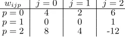
EachDCm transforms each value ofs(m) toop(m). In Equation 2, a specific example is given for

use with four input signals, with one signal per category and consists of some additional components. Additionally, the j 6= 3 component implies that signal category index is not summed with the other three signal categories i.e. inflammation is not treated in the same manner as the other signals, as shown in this equation. The interrelationships between the weights, determined through practical immunology, are shown in Table 2.

1 2 3 4 5 6 7 8 9 10 11 12 13 14 15 16 17 18 19 20 21 22 23 24 25 26 27 28 29 30 31 32 33 34 35 36 37 38 39 40 41 42 43 44 45 46 47 48 49 50 51 52 53 54 55 56 57 58 59

Table 2 Derivation and interrelationship between weights in the signal processing equation, where the values of the PAMP weights are used to create all other weights relative to the PAMP weight.W1 is the weight to transform the PAMP signal to the CSM output signal andW2 is the weight to transform the PAMP signal to the mature output signal.

wijp j= 0 j= 1 j= 2

p= 0 W1 W1

2 W1∗1.5

p= 1 0 0 1

p= 2 W2 W2

2 -W2∗1.5

An antigen store is constructed for use within the tissue cycle where all DCs in the population can collect antigen.

The cell update component maintains all DC data structures including the DC population of set sizeM. Each DC has an input signal matrix, antigen vector, cumulative output signals and migration threshold. The internal values ofDCm are updated, based on current data in the tissue signal matrix

and antigen vector. The DC input signals,s(m) use the identical mapping for signal categories as tissue s and are updated every cell cycle iteration. Each s(m) for DCm is updated via an overwrite every

cell cycle. These values are used to calculate output signal values, op(m), for DCm, which are added

cumulatively over a number of cell cycles to form ¯op(m), wherep= 0 is costimulatory value, p= 1 is

the semi-mature DC output signal andp= 2 is the mature DC output signal. With each cell update, DCs sampleRantigens from the tissue antigen vector A.

After the internal values of a DC are updated,o0is assessed againsttmthe cell’s migration threshold.

If o0 is greater than tm, the DC is ‘removed’ from the tissue. Here, ‘remove’ means that the DC is

de-allocated the receptors needed to sample the signal matrix and to collect antigen. On the next update cycle, the remaining output signals are checked and the analysis procedure is initiated.

In this implementation, each DC is assigned a random value fortm, within a specified range. The

random value adds some diversity to the DC population. The value of o0 is increased on exposure

to any signal and proportionately to the strength of the input signal. By using randomly assigned migration thresholds, each DC samples the signal matrix a different number of times throughout its lifetime. Some exist for a short period sampling once or twice, others can persist for longer, dependent on the strength of the signals. This creates a variable time window effect for the sampling.

Pseudocode for this specific instantiation of the DCA is given in Algorithm 1. This pseudocode shows both the update of the tissue and the individual DCs. The stages of the algorithm are shown, namely initialisation, update and analysis. While this provides the detail of the DC update mechanisms, this pseudocode does not encapsulate the asynchronous nature of the update stages. As libtissue is a multithreaded framework, the three updates are controlled by three different processes, therefore, the three updates occur asynchronously. This architecture is particularly suited for real time data processing as updates occur as and when they are required.

3.6 Antigen Aggregation

OnceDCmhas been removed from the population, the contents ofa(m) and values ¯op(m) are logged

to a file for the aggregation stage. Once completed, s(m), a(m) and ¯op(m) are all reset and DCm is

returned to the sampling population. The re-cycling of DCs continues until the stopping condition is met (l =L). Once all data has been processed by the DCs, the output log of antigen-plus-context is analysed.

The same antigen is presented multiple times with different context values. This information is recorded in a log file. The total fraction of mature DCs presenting said antigen (where ¯o1 > o¯2) is

divided by the total amount of times the antigen was presented namely ¯o1/(¯o1+ ¯o2). This is used to

1 2 3 4 5 6 7 8 9 10 11 12 13 14 15 16 17 18 19 20 21 22 23 24 25 26 27 28 29 30 31 32 33 34 35 36 37 38 39 40 41 42 43 44 45 46 47 48 49 50 51 52 53 54 55 56 57 58 59

input :T ={S, A}

output:aand context create DCs;

initialise parameters{I, J, K, L, M, N, O, P, Q}; forl < Ldo

updateAandS; form= 0toM do

forn= 0toQdo

DCmsamplesQantigen fromA;

end

for i= 0toI andj= 0toJdo

sDC ij =sij;

end

for n= 0toN do

DCmprocessesan(m);

end

forptoP do computeop;

¯

op(m) = ¯op(m) +op;

end

if o0(m)> tmthen

DCmremoved from population;

DCmmigrate, print antigen and context; DCmreset antigen vector and all signals;

end end

l++; end

analyse antigen and calculate MCAV

Algorithm 1: Pseudocode of the implemented DCA

3.7 Signals and Antigen

An integral part of DC function is the ability to combine multiple signals to produce context informa-tion. The semantics of the different categories of signal are derived from the study of the influence of the different signals on DCsin vitro. Definitions of the characteristics of each signal category are given below, with an example of an actual signal per category. This categorisation forms the signal selection schema. Any number of sources of information can be mapped using the outlined principles.

– PAMP -si0,e.g. the number of error messages generated per second by a failed network connection:

1. a signature of abnormal behaviour, e.g. an error message;

2. a high degree of confidence of abnormality associated with an increase in this signal strength. – Danger signal -si1,e.g. the number of transmitted network packets per second:

1. measure of an attribute which significantly increases in response to abnormal behaviour; 2. a moderate degree of confidence of abnormality with increased level of this signal, though a low

signal strength can represent normal behaviour.

– Safe signal -si2 e.g. the inverse rate of change of number of network packets per second. A high rate of change equals a low safe signal level and vice versa:

1. a confident indicator of normal behaviour in a predictable manner or a measure of steady-behaviour;

2. measure of an attribute which increases signal concentration due to the lack of change in strength.

Signals, though interesting, are inconsequential without antigen. To a DC, antigen is an element which is carried and presented to a T-cell, without regard for the structure of the antigen. Antigenis

1 2 3 4 5 6 7 8 9 10 11 12 13 14 15 16 17 18 19 20 21 22 23 24 25 26 27 28 29 30 31 32 33 34 35 36 37 38 39 40 41 42 43 44 45 46 47 48 49 50 51 52 53 54 55 56 57 58 59

4 Self-Organizing Maps

4.1 Biological Inspiration for SOM

Various properties of the brain were used as an inspiration for a large set of algorithms and compu-tational theories known as neural networks. Such algorithms have shown to be successful, however a vital aspect of biological neural networks was omitted in the algorithm’s development. This was the notion of self-organization and spatial organization of information within the brain. In 1981 Kohonen proposed a method which takes into account these two biological properties and presented them in his SOM algorithm [46].

The SOM algorithm generates, usually, two dimensional maps representing a scaled version of n-dimensional data used as the input to the algorithm. These maps can be thought of as “neural networks” in the same sense as SOM’s traditional rivals, artificial neural networks (ANNs). This is due to the algorithm’s inspiration from the way that mammalian brains are structured and operate in a data reducing and self-organised fashion. Traditional ANNs originated from the functionality and interoperability of neurons within the brain. The SOM algorithm on the other hand was inspired by the existence of many kinds of “maps” within the brain that represent spatially organised responses. An example from the biological domain is the somatotopic map within the human brain, containing a representation of the body and its adjacent and topographically almost identical motor map responsible for the mediation of muscle activity [47].

This spatial arrangement is vital for the correct functioning of the central nervous system [40]. This is because similar types of information (usually sensory information) are held in close spatial proximity to each other in order for successful information fusion to take place as well as to minimise the distance when neurons with similar tasks communicate. For example sensory information of the leg lies next to sensory information of the sole.

The fact that similarities in the input signals are converted into spatial relationships among the responding neurons provides the brain with an abstraction ability that suppresses trivial detail and only maps most important properties and features along the dimensions of the brain’s map [61].

4.2 SOM Algorithm Overview

As the algorithm represents the above described functionality, it contains numerous methods that achieve properties similar to the biological system. The SOM algorithm comprises of competitive learning, self-organization, multidimensional scaling, global and local ordering of the generated map and its adaptation.

There are two high-level stages of the algorithm that ensure a successful creation of a map. The first stage is the global ordering stage in which we start with a map of predefined size with neurons of random nature and using competitive learning and a method of self-organization, the algorithm produces a rough estimation of the topography of the map based on the input data. Once a desired number of input data is used for such estimation, the algorithm proceeds to the fine-tuning stage, where the effect of the input data on the topography of the map is monotonically decreasing with time, while individual neurons and their close topological neighbours are sensitised and thus fine tuned to the present input.

The original algorithm developed by Kohonen comprises of initialisation followed by three vital steps which are repeated until a condition is met:

– Choice of stimulus – Response

– Adaptation

Each of these steps are described in detail in the next section.

4.3 Algorithmic Detail and Implementation

1 2 3 4 5 6 7 8 9 10 11 12 13 14 15 16 17 18 19 20 21 22 23 24 25 26 27 28 29 30 31 32 33 34 35 36 37 38 39 40 41 42 43 44 45 46 47 48 49 50 51 52 53 54 55 56 57 58 59

due to their limited speed and integratability. For this reason a C++ based implementation is developed according to the original incremental SOM algorithm as described by Kohonen [48]. In this section a detailed analysis of the implemented algorithm and its step by step functional description follows.

4.3.1 Initialisation

A number of parameters have to be chosen before the algorithm is to begin execution. These include the size of the map, its shape, the distance measure used for comparing how similar nodes are, to each other and to the input feature vectors, as well as the kernel function used for the training of the map. Kohonen suggested recommended values for these parameters [47], which are used throughout our experiments. The values used in this paper are described in Section 5, found in Table 8. Once these parameters are chosen, a map is created of the predefined size, populated with nodes, each of which is assigned a vector of random values, wi, where idenotes node to which vectorwbelongs.

4.3.2 Stimulus Selection

The next step in the SOM algorithm is the selection of the stimulus that is to be used for the generation of the map. This is done by randomly selecting a subset of input feature vectors from a training data set and presenting each input feature vector, x, to the map, one item per epoch. An epoch represents one complete computation of the three vital steps of the algorithm.

4.3.3 Response

At this stage the algorithm takes the presented input,xand compares it against every nodei within the map by means of a distance measure betweenxand each nodes’ weight vectorwi. For example this

can be the Euclidean distance measure shown in Equation 3, where||.|| is the Euclidean norm andwi

is the weight vector of nodei. This way a winning node can be determined by finding a node within the map with the smallest Euclidean distance from the presented vector x, here signified byc.

c=argmin{||x−wi||} (3)

4.3.4 Adaptation

Adaptation is the step where the winning node is adjusted to be slightly more similar to the inputx. This is achieved by using a kernel function, such as the Gaussian function (hci) as seen in Equation 4

as part of a learning process.

hci(t) =α(t).exp

−||rc−ri||

2

2σ2_(t)

(4)

In the above function, α(t) denotes a “learning-rate factor” and σ(t) denotes the width of the neighbourhood affected by the Gaussian function. Both of these parameters decrease monotonically over time (t). During the first 1,000 steps, α(t) should have reasonably high values (e.g. close to 1). This is called theglobal ordering stage and is responsible for proper ordering ofwi. For the remaining

steps,α(t) should attain reasonably small values (≥0.2), as this is the fine-tuning stage where only fine adjustments to the map are performed. Both rc and ri are location vectors of the winner node

(denoted by subscriptc) andirespectively, containing information about a node’s location within the map.

wi(t+ 1) =wi(t) +hci(t)[x(t)−wi(t)] (5)

The learning function itself is shown in Equation 5. Here the Gaussian kernel functionhciis responsible

1 2 3 4 5 6 7 8 9 10 11 12 13 14 15 16 17 18 19 20 21 22 23 24 25 26 27 28 29 30 31 32 33 34 35 36 37 38 39 40 41 42 43 44 45 46 47 48 49 50 51 52 53 54 55 56 57 58 59

4.3.5 Repetition

Stimulus selection, Response and Adaptation are repeated a desired number of times or until a map of sufficient quality is generated. For our experiment this was set to a value suggested by Kohonen [48]. He states that the number of steps should be at least 500 times the number of map units. For this reason 100,000 epochs were used in our experiments. Another possible mechanism for the termination of the algorithm is the calculation of the quantization error, which is the mean of ||x−wc|| over the

training data. Once the overall quantization error falls below a certain threshold, the execution of the algorithm can stop as an acceptable lower dimensional representation of the input data has been generated.

5 Experimental Comparison

5.1 Scenarios

For the experiments in this paper, two data sets are compiled, collected using a system of signal collection scripts with raw input signal data collected from the Linux/proc filesystem. One data set is termed passive normal (PN) and contains a SYN scan performed without normal processes invoked by a user i.e. scan and shell processes. The second data set is termed active normal (AN). This data set contains an identical SYN scan but is combined with simultaneous instances of normal programs which are used actively by a user throughout the duration of the session i.e. scan, shell processes and a firefox web browser.

Block scans are conducted across 254 IP addresses connecting to multiple ports on each host successfully probed. Approximately 70 hosts out of the 254 addresses scanned are available at any one instance during the scan. For these scenarios, the DCA resides on a client machine which is connected to the main network. As the scanned local hosts are part of a university network and the availability of the hosts is beyond direct control, with the exception of the host on which the DCA monitors. The scan performed in both data sets is a standard SYN scan, with a fast probe sending rate (<0.1 seconds per probe), facilitated through the use of the popular scanning tool, nmap [17]. The command invoked to perform the SYN scan using nmap is “nmap -sS -v xxx.xxx.xxx.1-254”.

The AN data set is 7,000 seconds in duration, with ‘normal’ antigen generated by running a web browser over a separate remote ssh session. During browsing, multiple downloads, chat sessions and the receipt of e-mail occur representing different patterns of network behaviour. This actively generated network traffic is provided to observe if the algorithms can differentiate between two highly active processes which run simultaneously and modify the networking behaviour of the victim host. Having both normal and anomalous processes running via the monitored ssh demon may make the detection of the scan more difficult. This may increase the MCAV for the normal processes as the DCA relies on the temporal correlation of signals and antigen to perform detection.

The PN data set is also 7,000 seconds in duration and comprises of a SYN scan and its pseudo-terminal slave (pts) parent process as anomalous examples. The ssh demon process acts as normal antigen and is needed to facilitate the remote login. In addition, a firefox browser runs throughout the session, but the system calls are run locally and not through the ssh demon. Therefore this does not form antigen, but can influence the input signal data.

5.2 Data Pre-processing and Signals

The DCA relies on correct mapping of signals, ensured through the examination of preliminary samples of input data. For the detection of SYN scans, seven signals are derived from behavioural attributes of the victim host: two PAMPs, two danger signals, two safe signals and one inflammatory signal. Having multiple signals per category may make the DCA more robust against random network fluctuations or conversely could impede classification through conflicting inputs.

1 2 3 4 5 6 7 8 9 10 11 12 13 14 15 16 17 18 19 20 21 22 23 24 25 26 27 28 29 30 31 32 33 34 35 36 37 38 39 40 41 42 43 44 45 46 47 48 49 50 51 52 53 54 55 56 57 58 59

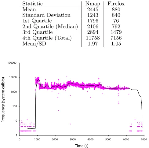
signal values are shown when the changes are small in magnitude. The inflammatory signal is simplified to a binary signal i.e. inflammation present (1) or not (0). All PAMPs, danger and safe signals are normalised within a range of zero to 100. A sketch of the input signals throughout the duration of the two sessions are shown in Figures 7, 8 and 9 for the AN data set and in Figure 10, 11 and 12 for the PN data set.

To devise a set of appropriate signals a number of preliminary experiments must be performed, in addition to the acquisition of knowledge regarding the effects of scanning and normal networking usage within a host. Initially a plethora of system variables are monitored under a variety of situations. The signals used in this experiment are network based attributes. This kind of system data appears to be the most variable under scanning conditions. Once the candidate signals are selected, they are then categorised using the general principles of signal selection i.e. PAMPs are signature-based, danger signals are normal at low values and anomalous at high values etc. Following the categorisation, the raw values of signals are transformed into normalised signals.

PAMP-1is the number of ICMP ‘destination unreachable’ (DU) error messages received per second.

Scanning IP addresses attached to hosts which are firewalled against ICMP packets generate these error messages in response to probing. This signal is shown to be useful in detecting ping scans and may also be important for the detection of SYN scans, as an initial ping scan is performed to find running hosts. In this experiment, the number of ICMP messages generated is significantly less than observed with a ping scan. To account for this, normalisation of this signal includes multiplying the raw signal value by five, capped at a value of 100 (equivalent to 20 DU errors per second). This process is represented in Equation 6 whererawis the unmodified system data andsignal represents the normalised output signal. These terms apply to all equations described within this section.

signal=min{100, raw∗5} (6)

PAMP-2 is the number of TCP reset packets sent and received per second. Due to the nature of

the scan, a volume of RST packets are created in both port status cases; they are generated from the scanning host if ports are open and are generated by the remote hosts if ports are closed. RST packets are not usually present in any considerable volume, so their increased frequency is a likely sign of scanning activity. This signal is normalised linearly, with a maximum cap set at 100 RSTs per second. This normalisation process is shown in Equation 7.

signal=min{100, raw} (7)

DS-1, the first danger signal is derived from the number of network packets sent per second. Previous experiments with this signal data indicate that it is useful for the detection of outbound scans [27]. A different approach is taken for the normalisation of this signal. A sigmoid function is used to emphasise the differences in observed rate, making the range of 100 to 700 packets per second more sensitive. This sensitive range is determined through preliminary data analysis of host behaviour during scans and normal use, with 750 packets per second found to be the median value across the plethora of preliminary data. This function makes the system less sensitive to fluctuations under 100 packets per second, whilst keeping the sensitivity of the higher values. A cap is set at 1500 packets per second, resulting in a signal range between 0 and 100. The general sigmoid function used for this transformation is shown in Equation 8, with the specific function shown in Equation 9.

f(x) = 1

1 +e−x (8)

signal=min{

₁

1 + 2(7.5−raw 100)

∗100,100} (9)

DS-2is derived from the ratio of TCP packets to all other packets processed by the network card of the scanning host. This may prove useful as during SYN scans there is a burst of traffic comprised of almost entirely TCP type packets, which is not usually observed under normal conditions. The ratio is normalised through multiplication by 100, to give this signal the same range as DS-1. This procedure is shown in Equation 10.

signal=

_{rawSignalT cp}

rawSignalAllP kts

1 2 3 4 5 6 7 8 9 10 11 12 13 14 15 16 17 18 19 20 21 22 23 24 25 26 27 28 29 30 31 32 33 34 35 36 37 38 39 40 41 42 43 44 45 46 47 48 49 50 51 52 53 54 55 56 57 58 59

0 1000 2000 3000 4000

0 20 40 60 80 100

Time(s)

Normalised Signal Value

− −

PAMP−1 PAMP−2

Fig. 7 Line graph of the PAMP (PAMP-1, PAMP-2) signals which constitute the AN (active normal) data set.

0 1000 2000 3000 4000

0 20 40 60 80 100

Time(s)

Normalised Signal Value

− −

DS−1 DS−2

Fig. 8 Line graph of the danger (DS-1, DS-2) signals which constitute the AN (active normal) data set.

0 1000 2000 3000 4000

0 20 40 60 80 100

Time(s)

Normalised Signal Value

− −

SS−1 SS−2

1 2 3 4 5 6 7 8 9 10 11 12 13 14 15 16 17 18 19 20 21 22 23 24 25 26 27 28 29 30 31 32 33 34 35 36 37 38 39 40 41 42 43 44 45 46 47 48 49 50 51 52 53 54 55 56 57 58 59

0 1000 2000 3000 4000

0 20 40 60 80 100

Time(s)

Normalised Signal Value

− −

PAMP−1 PAMP−2

Fig. 10 Line graph of the PAMP (PAMP-1, PAMP-2) signals which constitute the PN (passive normal) data set.

0 1000 2000 3000 4000

0 20 40 60 80 100

Time(s)

Normalised Signal Value

− −

DS−1 DS−2

Fig. 11 Line graph of the danger (DS-1, DS-2) signals which constitute the PN (passive normal) data set.

0 1000 2000 3000 4000

0 20 40 60 80 100

Time(s)

Normalised Signal Value

− −

SS−1 SS−2

1 2 3 4 5 6 7 8 9 10 11 12 13 14 15 16 17 18 19 20 21 22 23 24 25 26 27 28 29 30 31 32 33 34 35 36 37 38 39 40 41 42 43 44 45 46 47 48 49 50 51 52 53 54 55 56 57 58 59

Table 3 Ranges used in the normalisation function of SS-2.

Range Signal Value

40 - 45 0

46- 50 10

51- 60 50

61 + 100

SS-1is the rate of change of network packet sending per second. Safe signals are implemented to counteract the effects of the other signals, hopefully reducing the number of false positive antigen types. High values of this signal are achieved if the rate is low and vice versa. This implies that a large volume of packets can be legitimate, as long as the rate at which the packets are sent remains constant. The value for the rate of change can be calculated from the raw DS-1 signal value, though conveniently, the proc file system also generates a moving-average representation of the rate of change of packets per second (over 2 seconds). This raw value can be normalised between values of 10 and 100 and inverted so that the safe signal value decreases as the raw signal value increases. This normalisation process is described in Equation 11.

signal=min{100, max{0,(100−raw)∗10

9 }} (11)

SS-2is based on the observation that during SYN scans the average network packet size reduces to a size of 40 bytes, with a low standard deviation. Preliminary observations under normal conditions show that the average packet size for normal traffic is within a range of 70 and 90 bytes. A step function is implemented to derive this signal with transformation values presented in Table 3. Preliminary experiments have also shown that a moving average is needed to increase the sensitivity of this signal. This average is created over a 60 second period.

The inflammatory signal is binary and based on the presence of remote root logins. If a root log-in is detected through the monitored ssh demon, this signal is assigned a value of one. When used in the signal processing equation, this multiplies the resultant values of the other signals by two, acting as an amplifier for all other signals including the safe signal. This signal may be useful as to perform a SYN scan the invocation has to come from a user with root privileges. While this is a very important feature of the SYN scan process, it is not suitable for use as a PAMP signal as it can be easily spoofed. Thorough analysis of the relationship between inflammation and the DCA is outside of the scope of this paper and may feature in future work. While this signal influences the rates of migration of the DCs, it does not influence the rates of detection as the addition of this signal increases the output signal values for both the semi-mature output (o1) and the mature output (o2) signals.

As shown in Figure 7-9 and 10-12, the AN signals are more variable than the PN signals, as many more processes run during the AN session. In the AN session, the nmap scan is invoked at 651 seconds. Signals PAMP-1, PAMP-2 and DS-2 clearly change for the duration of the scan. The remaining signals are less clear, though some evidence of changes throughout the scan duration is shown. The changes are transient and localised in particular to the beginning of the scan, when the majority of probes are sent to other hosts.

The signals of the PN data set are less noisy. Analysis of input antigen confirms nearly 99% of these antigen belong to the anomalous pts and nmap processes. PAMP-1 and PAMP-2 are responsive to the scan, as shown by their rapid decline towards the end of the scanning period, at 5,500 seconds. Changes in DS-1 are more pronounced in the PN data set, yet the magnitude of this signal is smaller than expected. DS-2 appears to be highly correlated with the scan, yielding values of over 20 throughout the scan duration. SS-1 performs poorly and only decreases in response to the scan in a few select places. SS-2 falls sharply in the middle of the scan, as predicted, but otherwise remains at a constant level of 60 even after the scan has finished.

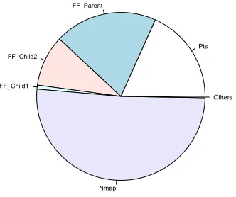
5.3 Antigen